What is Cook’s theorem?

In order to provide a reasonable basis for P-reduciblility in Theorem 1, Cook introduced a tool called query machine, which is a mix of an oracle and a deterministic Turing machine, to replace a nondeterministic Turing machine. It is this query machine that sows the seeds of confusion of $NDTM$ (NonDeterministic Turing Machine) and $DTM$ (Deterministic Turing Machine) in the proof of Theorem 1.

Let us analyze this query machine. A query machine was defined in [1]:

A query machine is a multitape Turing machine with a distinguished tape called the query tape, and three distinguished states called the $query~state$, $yes~state$, and $no~state$, respectively. If $M$ is a query machine and $T$ is a set of strings, then a $T$-computation of $M$ is a computation of $M$ in which initially $M$ is in the initial state and has an input string $w$ on its input tape, and each time $M$ assures the query state there is a string $u$ on the query tape, and the next state $M$ assumes is the yes state if $u\in T$ and the no state if $u\not\in T$. We think of an ’oracle’, which knows $T$, placing $M$ in the yes state or no state.

Then the concept of P-reduciblility was defined based on query machine [1]:

Definition. A set S of strings is P-reducible (P for polynomial) to a set T of strings iff there is some query machine M and a polynomial Q(n) such that for each input string w, the T-computation of M with input w halts within Q($\mid w\mid$) steps ($\mid w\mid$ is the length of w) and ends in an accepting state iff $w\in S$.

It is not hard to see that P-reducibility is a transitive relation. Thus the relation $E$ on sets of strings, given by $(S,T)\in E$ iff each of $S$ and T is P-reducible to the other, is an equivalence relation. The equivalence class containing a set S will be denoted by deg (S) (the polynomial degree of difficulty of S).

In addition, five $NP$ problems were given as examples to illustrate $S$ and $T$ [1]:

We now define the following special sets of strings.

1. 1.

   The subgraph problem is the problem given two finite undirected graphs, determine whether the first is isomorphic to a subgraph of the second. A graph G can be represented by a string G on the alphabet $\{0,1,*\}$ by listing the successive rows of its adjacency matrix, separated by $*$s. We let subgraph pairs denote the set of strings $\overline{G}_{1}\ast\ast\overline{G}_{2}$ such that $G_{1}$ is isomorphic to a subgraph of $G_{2}$.

2. 2.

   The graph isomorphism problem will be represented by the set, denoted by $\{$isomorphic graph pairs$\}$, of all strings $\overline{G}_{1}\ast\ast\overline{G}_{2}$ such that $G_{1}$ is isomorphic to $G_{2}$.

3. 3.

   The set $\{$Primes$\}$ is the set of all binary notations for prime numbers.

4. 4.

   The set $\{$DNF tautologies$\}$ is the set of strings representing tautologies in disjunctive normal form.

5. 5.

   The set D3 consists of those tautologies in disjunctive normal form in which each disjunct has at most three conjuncts (each of which is an atom or negation of an atom).
   

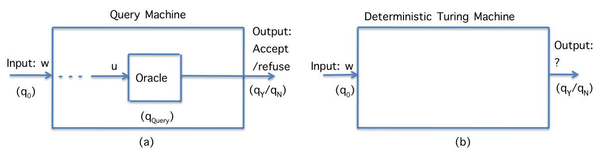
We interpret how a query machine $M$ accepts an instance $w$ of an $NP$ problem in polynomial time, which is illustrated in Fig. 1(a).

$S$ refers to a set of strings that represents all instances that have solutions, for example, $S$ refers to a set of instances $\overline{G}_{1}\ast\ast\overline{G}_{2}$ of the graph isomorphism problem such that $G_{1}$ is isomorphic to $G_{2}$. $T$ refers to a set of formulas in $DNF$ that are tautologies.

Initially, $M$ is in the initial state $q_{0}$ and has $w$ representing an instance of a $NP$ problem as input. Then, $M$ assures the query state $q_{Query}$ where there is a string $u$ representing a formula in $DNF$ as input for an oracle and this oracle instantly determines whether $u\in T$, that is, whether $u$ is tautology. Finally, according to the obtained reply, if $u\in T$ then the oracle places $M$ in the yes state $q_{Y}$ and accepts $w$; or if $u\not\in T$ then the oracle places $M$ in the no state $q_{N}$ and refuses $w$.

In this way, $S$ is said to be $P$-reducible to $T$.

Therefore, a query machine is in fact a formalized oracle. But it should pay special attention to the essence of oracle. The existence of an oracle is just a hypothesis rather than a fact, so it is just theoretically valid, but not in practice, while a deterministic Turing machine is either theoretically or practically valid. That is, oracle and $DTM$ are two concepts situated at different levels (see Fig. 1).

Unfortunately, it seems that Cook did not realize this fundamental difference, when he interpreted $P$-reducibility in [1]:

By reduced we mean, roughly speaking, that if tautology hood could be decided instantly (by an ”oracle”) then these problems could be decided in polynomial time. In order to make this notion precise, we introduce query machines, which are like Turing machines with oracles in [1].

In other words, Cook made a direct logic deduction between oracle and $DTM$, but this is a question begging, because the existence of an oracle itself needs to be proved. It is this cognitive bias that leads to the confusion of query machine and $DTM$, thus the confusion of $NDTM$ and $DTM$ in the proof of Theorem 1.

The proof of Theorem 1 consists in constructing $u$ from $w$, where $w$ is an instance of an $NP$ problem and $u$ is a formula $A(w)$ in $CNF$ (see Fig. 1(a)), through representing a computation of a nondeterministic Turing machine for $w$.

This idea was explained in [1]:

Suppose a nondeterministic Turing machine $M$ accepts a set $S$ of strings within time $Q(n)$, where $Q(n)$ is a polynomial. Given an input $w$ for $M$, we will construct a propositional formula $A(w)$ in conjunctive normal form ($CNF$) such that $A(w)$ is satisfiable iff $M$ accepts $w$.

However, the construction of $A(w)$ is a deterministic and polynomial time process, so Cook discretely replaced a nondeterministic Turing machine by a deterministic Turing machine through a query machine (see Fig. 1).

We interpret how it could happen.

Originally the above $M$ refers to a nondeterministic Turing machine, but this $M$ has discretely changed in the following [1]:

We may as well assume the Turing machine has only on tape, which is infinite to the right but has a left-most square. Let us number the squares from left to right $1,2,\dotsc$ Let us fix an input $w$ to $M$ of length $n$, and suppose $w\in S$. Then there is a computation of M with input w that ends in an accepting state within $T=Q(n)$ steps. The formula $A(w)$ will be built from many different proposition symbols, whose intended meaning, listed below, refer to such a computation.

That is, $A(w)$ is built to represent a computation of $M$. Let us interpret the meaning of this computation through the analysis of the construction of $A(w)$ [1]:

Suppose the tape alphabet for $M$ is $\{\sigma_{1},\dotsc,\sigma_{l}\}$ and the set of states is $\{q_{1},\dotsc,q_{r}\}$. Notice that since the computation has at most $T=Q(n)$ steps, no tape square beyond $T$ is scanned.

Proposition symbols :

• •

  $P_{s,t}^{i}$ for $1\leq i\leq l$, $1\leq s,t\leq T$. $P_{s,t}^{i}$ is true iff tape square number $s$ at step $t$ contains the symbol $\sigma_{i}$.

• •

  $Q_{t}^{i}$ for $1\leq i\leq r$, $1\leq t\leq T$. $Q_{t}^{i}$ is true iff at step t the machine is in state $q_{i}$.

• •

  $S_{s,t}$ for $1\leq s,t\leq T)$ is true iff at step $t$ square number $s$ is scanned by the tape head.

The formula $A(w)$ is a conjunction $B\land C\land D\land E\land F\land G\land H\land I$ formed as follows. Notice A(w) is in conjunctive normal form.

B will assert that at each step t, one and only one square is scanned. B is a conjunctive ${B_{1}\land B_{2}\land\dotsc\land B_{T}}$, where $B_{t}$ asserts that at time t one and only one square is scanned :

$B_{t}=(S_{1,t}\lor S_{2,t}\lor,\dotsc\lor S_{T,t})\land\big[\bigwedge_{1\leq i<j\leq Q(n)}(\neg S_{i,t}\lor\neg S_{j,t})\big].$

For $1\leq s\leq T$ and $1\leq t\leq T$, $C_{s,t}$ asserts that at square $s$ and time $t$ there is one and only one symbol. $C$ is the conjunction of all the $C_{s,t}$.

$D$ asserts that for each $t$ there is one and only one state.

$E$ asserts the initial conditions are satisfied :

$E=Q_{1}^{0}\land S_{1,1}\land P_{1,1}^{i_{1}}\land P_{2,1}^{i_{2}}\land\dotsc\land P_{n,1}^{i_{n}}\land P_{n+1,1}^{1}\dotsc\land P_{T,1}^{1}$

Where $w=\sigma_{i_{1}},\dotsc,\sigma_{i_{n}}$ , $q_{0}$ is the initial state and $\sigma_{1}$ is the blank symbol.

$F$, $G$, and $H$ assert that for each time $t$ the values of the $P^{\prime}$s, $Q^{\prime}$s and $S^{\prime}$s are updated properly. For example, $G$ is the conjunction over all $t$, $i$, $j$ of $G_{i,j}^{t}$, where $G_{i,j}^{t}$ asserts that if at time $t$ the machine is in state $q_{i}$ scanning symbol $\sigma_{j}$, then at time $t+1$ the machine is in the state $q_{k}$, where $q_{k}$ is the state given by the transition function for $M$.

$G_{i,j}^{t}=\bigwedge_{s=1}^{T}(\neg Q_{t}^{i}\lor\neg S_{s,t}\lor\neg P_{s,t}^{j}\lor Q_{t+1}^{k}).$

Finally, the formula $I$ asserts that the machine reaches an accepting state at some time. The machine $M$ should be modified so that it continues to compute in some trivial fashion after reaching an accepting state, so that $A(w)$ will be satisfied.

Firstly, let us clarify $M$. Notice that $B$, $C$, $D$ and $I$ refer to just the physical structure of $M$; $F$, $G$ and $H$ refer to the transition function of $M$; and $E$ concerns the initial condition of a computation of $M$.

Such a computation proceeds as below. Starting from $E$, the assignment of the proposition symbols corresponding to following steps are deduced out according to $B\land C\land D\land F\land G\land H$, finally the truth of $I$ is deduced out in polynomial time. Since this computation ends in polynomial time $Q(n)$, and $F$, $G$ and $H$ represent the transition function of $M$ in terms of $G_{i,j}^{t}=\bigwedge_{s=1}^{T}(\neg Q_{t}^{i}\lor\neg S_{s,t}\lor\neg P_{s,t}^{j}\lor Q_{t+1}^{k})$, then this computation is in fact a computation of a deterministic Turing machine $M$. In other words, the original nondeterministic Turing machine $M$ has been discretely transformed into a deterministic Turing machine $M$!

Then, we interpret the meaning of such a computation by clarifying $E$. $E$ refers to the assignment of the proposition symbols corresponding to the initial time $t=1$, $E=Q_{1}^{0}\land S_{1,1}\land P_{1,1}^{i_{1}}\land P_{2,1}^{i_{2}}\land\dotsc\land P_{n,1}^{i_{n}}\land P_{n+1,1}^{1}\dotsc\land P_{T,1}^{1}$, where $Q_{1}^{0}$ means that $M$ is in the initial state $q_{0}$, $S_{1,1}$ means that the tape head scans square number 1, $P_{n+1,1}^{1}\dotsc\land P_{T,1}^{1}$ refers to the blank symbols $\sigma_{1}$ after $\sigma_{i_{1}},\dotsc,\sigma_{i_{n}}$, and $P_{1,1}^{i_{1}}\land P_{2,1}^{i_{2}}\land\dotsc\land P_{n,1}^{i_{n}}$ refers to a string $\sigma_{i_{1}},\dotsc,\sigma_{i_{n}}$ on the tape that is claimed to refer to an instance $w$ of a problem.

That is to say, given an instance $w$ of an $NP$ problem, a deterministic Turing machine $M$ determines whether to accept $w$ in polynomial time, and $A(w)$ is built to represent this computation (see Fig. 1(b)).

In other words, the proof of Theorem 1 claims that a deterministic Turing machine can accept $w$ like a nondeterministic Turing machine, that is, $NDTM$ is confused with $DTM$ by means of query machine!

References

- [1] Stephen Cook, The complexity of theorem proving procedures. Proceedings of the Third Annual ACM Symposium on Theory of Computing. pp. 151–-158 (1971).
- [2] http://en.wikipedia.org/wiki/NP_(complexity)
- [3] Michael Sipser, Introduction to the Theory of Computation, Second Edition. International Edition (2006).
- [4]
Stephen Cook, The P versus NP Problem. Clay Mathematics Institute.
http://www.claymath.org/millennium/P_vs_NP/pvsnp.pdf. - [5] Michael R. Garey, David S. Johnson, Computers and Intractability: A Guide to the Theory of NP-Completeness. W. H. Freeman and company (1979).
- [6]
William I. Gasarch, The P=?NP poll. SIGACT News Complexity Theory Column 74.
http://www.cs.umd.edu//~gasarch/papers/poll2012.pdf. - [7] Yu Li, What is NP? - Interpretation of a Chinese paradox white horse is not horse. (to appear)
- [8] http://en.wikipedia.org/wiki/CookLevin_theorem
- [9]
JianMing Zhou, Computability vs. Nondeterministic and P vs. NP.
http://arxiv.org/abs/1305.4029. - [10] Scott Aaronson, Why Philosophers Should Care About Computational Complexity, Electronic Colloquium on Computational Complexity, Revision 2 of Report No. 108 (2011).