Scale invariance implies conformal invariance for the three-dimensional Ising model

Conformal symmetry plays a considerable role both in high energy and condensed matter physics. There has been a renewed interest in recent years, particularly because of the AdS/CFT conjecture [1] and the successful use of conformal methods in three-dimensional critical physics [2, 3, 4, 5, 6, 7]. The groundbreaking papers of the 1970s and 1980s [8, 9, 10, 11, 12, 13] solved two fundamental issues in two dimensions: First, scale invariance implies conformal invariance under mild assumptions [12, 13] and, second, conformal symmetry enables us to solve most of the scale invariant problems that is, to determine critical exponents and correlation functions [14].

An important ingredient for the exact solution of two-dimensional conformal models is the existence of an infinite number of generators of the conformal group. In higher dimensions, the number of generators is finite, and we could naively conclude that symmetry arguments alone are not sufficient to solve a model in the critical regime. However, it is well-known that scale-invariant theories are in a one-to-one correspondence with the fixed points of the Wilson Renormalization Group (RG) [15], and that the fixed point of a theory completely determines all the correlation functions of a critical model for sufficiently small wavenumbers. Therefore, at the level of principles, scale (and a fortiori conformal) invariance is sufficient to determine all the universal critical properties of a model. Of course, in practice, the computation of these critical properties requires us to solve the functional Wilson RG equations. This is a formidable task that we do not know how to carry out without approximations. Any supplementary information, even if redundant, is therefore welcome and this is what conformal invariance could provide. A breakthrough in this direction has been achieved these last years with the conformal bootstrap program [2, 3, 4], which led to the exact (although numerical) computation of the critical exponents of the Ising model in three dimensions assuming, among other things, conformal invariance.

In parallel, a large activity has been devoted to understanding the relation between scale and conformal invariance in – or close to – four dimensions. It has been proven to all orders of perturbation theory that scale invariance implies conformal invariance [16] in four-dimensional unitary and Poincaré invariant theories. Moreover, there are strong indications that a non-perturbative proof could be at reach in this dimension [17, 18, 19].

Despite decades of effort, it is still an open question to know whether a typical statistical model is conformally invariant at criticality in three dimensions. The aim of this article is twofold. First, we derive a sufficient condition which, when fulfilled, ensures that scale invariance implies conformal invariance. In the second part of the paper, we prove that this condition is fulfilled in any dimension for the euclidean $\mathbb{Z}_{2}$ model.

The rest of the paper is organized as follows. In Sect. II, we make a brief review of the nonperturbative renormalization-group. We then recall in Sect. III the relation between scale invariance and the NPRG. By using the same methods, we generalize these considerations to the case of conformal invariance in Sect. IV. In Sect. V, we finally derive a sufficient condition for the validity of conformal invariance in scale invariant models. We show, on general arguments that this condition is expected to be fulfilled in O($N$) models (and in generalizations thereof). In Sect VI, these considerations are made rigourous for the Ising universality class. We give our conclusions in Sect VII.

The proof of conformal invariance in all dimensions presented below is intimately related to the deep structure of the Wilson RG ¹¹ 1 The history of the relation between conformal invariance and Wilson RG is long, see for example [20, 21]. and scale invariance. We therefore start by recalling, in the case of the $\mathbb{Z}_{2}$ model, the formalism of the modern formulations (sometimes called Nonperturbative RG, or functional RG) of the Wilson RG [22, 23, 24, 25, 26]. The coarse-graining procedure at some RG scale $k$ is implemented by smoothly decoupling the long-wavelength modes $\varphi(|q|<k)$ of the system, also called the slow modes, by giving them a large mass, while keeping unchanged the dynamics of the short-wavelength/rapid ones $\varphi(|q|>k)$. This decoupling is conveniently implemented by modifying the action or the Hamiltonian of the model: $S[\varphi]\to S[\varphi]+\Delta S_{k}[\varphi]$ where $\Delta S_{k}[\varphi]$ is quadratic in the field and reads, in Fourier space, $\Delta S_{k}[\varphi]=1/2\int_{q}\,R_{k}(q^{2})\varphi(q)\varphi(-q)$. The precise shape of $R_{k}(q^{2})$ does not matter for what follows as long as it can be written as

where $Z_{k}$ is the field renormalization factor and $r$ is a function that, (i) falls off rapidly to 0 for $q^{2}>k^{2}$ – the rapid modes $\varphi(|q|>k)$ are not affected by $\Delta S_{k}$ – and (ii) goes to a constant for $q^{2}=0$ – the slow modes $\varphi(|q|<k)$ acquire a mass of order $k$ and thus smoothly decouple. The partition function, which now depends on the RG parameter $k$, reads:

where the field $J$ is a source term which corresponds to the magnetic field in the Ising model and where the ultra-violet (UV) regime of the functional integral is assumed to be regularized at a momentum scale $\Lambda$, see for instance [27] for a lattice regularization in this formalism. It is convenient to define the free energy ${\cal W}_{k}[J]=\ln{\cal Z}_{k}[J]$ and its (slightly modified) Legendre transform by

with $\phi(x)=\delta{\cal W}_{k}/\delta J(x)$, $R_{k}(|x-y|)$ the inverse Fourier transform of $R_{k}(q^{2})$ and where the last term has been added for the following reason. When $k$ is close to $\Lambda$, all modes are completely frozen by the $\Delta S_{k}$ term because, for all $q$, $R_{\Lambda}(q^{2})$ is very large. Thus, ${\cal Z}_{k\to\Lambda}$ can be computed by the saddle-point method and it is then straightforward to show that the presence of the last term in Eq. (3) leads to $\Gamma_{\Lambda}[\phi]\simeq S[\varphi=\phi]$. On the contrary, when $k=0$, the definition of $R_{k}$ implies that $R_{k=0}(q^{2})\equiv 0$ and the original model is recovered: ${\cal Z}_{k=0}[J]={\cal Z}[J]$ and $\Gamma_{k=0}[\phi]=\Gamma[\phi]$, with $\Gamma[\phi]$ the usual Gibbs free energy or generating functional of one-particle-irreducible correlation functions.

The exact RG equation for $\Gamma_{k}$ reads [23, 24, 25]:

where $t=\ln(k/\Lambda)$, and $G_{k,xy}[\phi]$ is the field-dependent propagator:

We now discuss how scale invariance emerges in the NPRG formalism. We first consider a scale-invariant model described by an action $S_{\rm scal}$. As we discuss in the following, the existence of such a model is not necessary for our proof but it is convenient to imagine that it exists to motivate the form of the expected Ward identity (WI) of scale invariance. If such a model existed, this WI would be obtained by performing the following infinitesimal change of variables $\varphi(x)\to\varphi(x)+\epsilon(D_{\phi}+x_{\mu}\partial_{\mu})\varphi(x)$ in the functional integral, with $D_{\phi}$ the scaling dimension of the field, usually written in terms of the anomalous dimension $\eta$ as $D_{\phi}=(d-2+\eta)/2$. Actually, the analysis of this model and of its WI faces both UV and infrared (IR) problems. In the IR regime, non-analyticities are present and, in the UV, it is difficult to control mathematically the continuum limit: $\Lambda\to\infty$. Let us first discuss the IR aspect. Since $\Delta S_{k}[\phi]$ acts as an IR regulator, the Wilson RG offers a solution to the IR problem: the regularized model, Eq. (2), is not scale invariant even if the original model associated with $S_{\rm scal}$ were and, thus, all $\Gamma_{k>0}^{(n)}(\{p_{i}\})$ are regular contrarily to $\Gamma_{k=0}^{(n)}(\{p_{i}\})$. The price to pay for regularity is the breaking of scale invariance that manifests itself through a modification of the WI [see [28, 29] for situations where $R_{k}$ breaks symmetries]. By enlarging the space of cutoff functions $R_{k}$ to arbitrary functions $R_{k}(x,y)$ that are neither constrained to satisfy (1) nor to be invariant under rotations and translations [as also done in [30]], this modified WI for scale invariance, obtained from Eqs. (2,3), reads

where $D^{x}=x_{\mu}\partial_{\mu}^{x}$ and $D_{R}=2d-2D_{\phi}$ is the scaling dimension of $R_{k}$ which implies that the field renormalization in Eq. (1) behaves as $Z_{k}\propto k^{-\eta}$. By constraining $R_{k}(q)$ to be of the form (1), Eq. (6) can be conveniently rewritten (following [29]):

Introducing dimensionless and renormalized quantities (denoted with a tilde)

Eq. (7) rewrites:

Eq. (11) means that an hypothetical scale-invariant action $S_{\rm scal}$ would lead, in its regularized and not scale-invariant version $S_{\rm scal}+\Delta S_{k}$, to a RG flow where $\tilde{\Gamma}_{k}[\tilde{\phi}]$ would be at a fixed point $\tilde{\Gamma}^{*}[\tilde{\phi}]$ for all values of $t$: $\partial_{t}\tilde{\Gamma}^{*}[\tilde{\phi}]=0$.

The very structure of the Wilson RG (or NPRG) also solves the UV problem. Actual models have a natural UV cutoff $\Lambda$ (e.g. a lattice spacing) at which is defined their microscopic action $S$. The momentum integrals are therefore cut-off at $\Lambda$ and are thus UV finite. At scales of order $\Lambda$ (i.e., if we consider correlation functions, in the regime where at least one external momentum or $k$ or the magnetic field in appropriate units, is of the order of $\Lambda$), the model is not scale invariant. In fact scale invariance is an emergent property that appears in the IR when some parameter (such as the temperature) has been fine-tuned. We call $S_{\rm crit}$ the corresponding action. In the RG formalism, scale invariance emerges in the IR regime when integrating the RG flow starting at $\Gamma_{\Lambda}[\phi]=S_{\rm crit}[\varphi=\phi]$ because $\tilde{\Gamma}_{k}$ gets close to a fixed point for large negative $t$, that is, $k\ll\Lambda$. As discussed above, the fixed-point condition coincides with the WI for scale invariance in presence of a regulator, see Eqs. (7,11). As a consequence, if the RG flow is attracted towards an IR fixed-point, then scale invariance emerges in the universal, long-distance regime ²² 2 A running anomalous dimension can be defined by $\eta_{k}=-\partial_{t}\log Z_{k}$. It is only around the fixed point that $\eta_{k}$ approaches a fixed-point value which is nothing else than $\eta$.. We stress that this discussion does not rely on the actual existence of a well-defined continuum limit associated with a scale-invariant action $S_{\rm scal}$ which is, per se, an interesting issue, but that we do not need to address in the present work.

When the microscopic action is slightly different from the critical one (e.g. choosing a temperature slightly away from the critical one), the RG trajectory approaches the fixed point and then stays close to it for a long RG “time”, before departing. In this situation, the correlation length $\xi$ is finite but large and the WI is almost fulfilled for momenta $\Lambda\gg p\gg\xi^{-1}$. This defines the critical regime of the theory. The closer the microscopic action is tuned to the critical one, the larger the correlation length $\xi$, and the better the WI is fulfilled.

Let us now make two comments. First, when $k\to 0$, $\partial_{t}\Gamma_{k}[\phi]$ becomes negligible compared to any $k$-independent finite scale and $\Gamma_{k}\to\Gamma$. In this limit, Eqs. (7,11) become the usual WI of scale invariance, as expected. Second, the above analysis shows that among the continuous infinity of solutions of the fixed point equation $\partial_{t}\tilde{\Gamma}_{k}[\tilde{\phi}]=0$, only those that are regular for all fields are acceptable since they must be the limit when $k\to 0$ of the smooth evolution of $\tilde{\Gamma}_{k}[\tilde{\phi}]$ from $S_{\rm crit}[\tilde{\phi}]$. There is generically only a discrete, often finite, number of such physical fixed-points.³³ 3 Two well-known exceptions to this rule are the line of fixed points of the $O(2)$ model in $d=2$ [31] and the discrete infinity of (multicritical) $Z_{2}$-invariant fixed points in $d=2$ [32, 33].

A characteristic feature of the physical fixed-points is that the linearized flow around them has a discrete spectrum of eigenvalues from which some critical exponents can be straightforwardly obtained [15]. The discrete character of the eigenperturbations around a fixed point has been studied intensively by perturbative means. As for the Wilson RG, it has been studied in detail in the particular case of the O$(N)$ models in [34, 35, 36]. Although obtained within the derivative expansion of the exact RG flow (4), its discrete character certainly remains true beyond this approximation. The eigenvalues $\lambda$ are obtained from the flow by substituting $\tilde{\Gamma}_{k}[\tilde{\phi}]\to\tilde{\Gamma}^{*}[\tilde{\phi}]+\epsilon\,\exp(\lambda t)\tilde{\gamma}[\tilde{\phi}]$ and retaining only the $O(\epsilon)$ terms. (With our definition of $t$, a relevant operator has a negative eigenvalue.) This leads to the eigenvalue problem

where $\tilde{x}_{i}=\{\tilde{x},\tilde{y},\tilde{z},\tilde{w}\}$, $\tilde{G}^{*}[\tilde{\phi}]$ is the dimensionless renormalized propagator at the fixed point: $\tilde{G}^{*}=(\tilde{\Gamma}^{*(2)}+r)^{-1}$ and $r(\tilde{x})$ is the dimensionless inverse Fourier transform of $r(q^{2}/k^{2})$ defined in Eq. (1).

We conclude from the above discussion that regularity selects among all the fixed-point functionals $\tilde{\Gamma}^{*}[\tilde{\phi}]$ those that are physical, that is, that can be reached by an RG flow from a physical action $S_{\rm crit}$ and that have a discrete spectrum of eigenperturbations.

Let us now study conformal invariance by following the same method as above. As in the case of scale invariance, to motivate the form of the WI we imagine that a conformally-invariant model, associated with an action $S_{\rm conf}[\varphi]$ written in terms of a primary field $\varphi$, exists. We put aside for now the problem of the existence of this model since, as discussed below, we do not need that it actually exists for our proof. If such a model existed, the modified WI would follow from performing the infinitesimal change of variables $\varphi(x)\to\varphi(x)+\epsilon_{\mu}(x^{2}\partial_{\mu}-2x_{\mu}x_{\nu}\partial_{\nu}+2\alpha x_{\mu})\varphi(x)$ in Eq. (2). By considering general cutoff functions as in Eq. (6), we find that it reads:

with $K_{\mu}^{x}=x^{2}\partial_{\mu}^{x}-2x_{\mu}x_{\nu}\partial_{\nu}^{x}$. By specializing $R_{k}$ to functions of the form Eq. (1) and requiring again that $Z_{k}~\propto~k^{-\eta}$, Eq. (13) can be rewritten

Again, this identity boils down to the usual WI of conformal invariance in the limit $k\to 0$ where $R_{k}\to 0$.

At any fixed point, the scaling dimension of $\Sigma_{k}^{\mu}[\phi]$ is fixed by Eq. (14) to be $-1$. We thus define $\tilde{\Sigma}_{k}^{\mu}[\tilde{\phi}]=k\,\Sigma_{k}^{\mu}[\phi]$. Its flow equation reads:

where $\tilde{\Sigma}^{\mu\,(2)}_{k}[\tilde{\phi}]$ is the second functional derivative of $\tilde{\Sigma}^{\mu}_{k}$.

An important property of $\Sigma_{k}^{\mu}$ is that, at the fixed point, it is the integral of a density with no explicit dependence on $x_{\mu}$. Indeed, observe that the left-hand-sides of Eqs. (6) and (13) can be interpreted as the action of the generators of dilatations $\mathcal{D}$ and conformal transformations $\mathcal{K}_{\mu}$ on $\Gamma_{k}$.

that is, $\Sigma_{\mu}=\mathcal{K}_{\mu}\Gamma_{k}$. Similar expressions can be obtained for the generators of translations $\mathcal{P}_{\mu}$ and rotations $\cal J_{\mu\nu}$:

It can easily be checked that the generators satisfy the algebra of the conformal group. In particular, applying $[\mathcal{P}_{\mu},\mathcal{K}_{\nu}]=2\delta_{\mu\nu}\mathcal{D}+2\mathcal{J}_{\mu\nu}$ to a translation, rotation and dilatation invariant $\Gamma_{k}$ yields

Thus, at the fixed point, $\Sigma_{k}^{\mu}$ is the integral of a density that does not have an explicit dependence on $x$. This density only depends on the field and its derivatives. This proof generalizes trivially to other scalar models.

Let us now consider a physical model at criticality. At the scale $\Lambda$, $\Gamma_{\Lambda}=S=S_{\rm crit}$ and the model is neither conformally nor scale invariant. However, when $k\ll\Lambda$, the regularized model gets close to a fixed point and thus $\tilde{G}_{k}\simeq\tilde{G}^{*}$ and $\tilde{\Sigma}_{k}^{\mu}[\tilde{\phi}]\simeq\tilde{\Sigma}^{\mu*}[\tilde{\phi}]$. The key point of our proof is that at the fixed point, Eq. (15) is identical to (12) with $\tilde{\gamma}[\tilde{\phi}]\to\tilde{\Sigma}^{\mu*}[\tilde{\phi}]$ and $\lambda=-1$ although these two equations have different physical meanings. A sufficient condition for proving conformal invariance is therefore to show that there is no integrated vector eigenperturbation $V_{\mu}=\int_{x}\mathcal{V}_{\mu}$ of $\tilde{\Gamma}^{*}[\tilde{\phi}]$ of scaling dimension $D_{V}=-1$. If no such eigenperturbation exists, the conformal WI is satisfied, which means that the system is conformally invariant at criticality in the long distance regime. Moreover, the form of the conformal WI (14) fixes the transformation law fulfilled by $\varphi$, which is the one of a primary field.

To understand how conformal invariance is related with the scaling dimension of the vector eigenperturbations, it proves useful to consider three simple examples. The first one is the Ising model in $d=4$. The fixed point being gaussian, the eigenvalues are trivially given by the canonical dimensions. By using the fact that $\tilde{\Sigma}^{\mu}_{k}$ is $\mathbb{Z}_{2}-$ and translation-invariant, see Eqs. (14) and (20), we find by inspection that the vector operator with lowest dimension reads $\int_{x}\phi\,\partial_{\mu}\phi(\partial\phi)^{2}$. It has therefore dimension +3. Note that there exists local vectors operators with lower scaling dimensions [$\phi\partial_{\mu}\phi$, $\phi^{3}\partial_{\mu}\phi$ and $\phi\partial_{\mu}\phi(\partial_{\nu}\phi)^{2})$]. However these are total derivatives and are not associated with integrated vector operators. In the absence of vector operator of dimension $-1$, we retrieve the well-known property that this model is conformally invariant at criticality in the long distance regime [13, 16]. Using standard methods, we can compute the corrections to the scaling dimension of the vector operator $\int_{x}\phi\,\partial_{\mu}\phi(\partial\phi)^{2}$ in a systematic expansion in $\epsilon=4-d$. We performed the calculation at one loop and found that the correction vanishes. The scaling dimension is therefore $3+\mathcal{O}(\epsilon^{2})$.

This analysis can be extended to the O($N$) models. In $d=4$, there exists now two independent integrated vector operators, $\int_{x}\phi^{a}(\partial_{\mu}\phi^{a})(\partial_{\nu}\phi^{b})^{2}$ and $\int_{x}\phi^{a}(\partial_{\nu}\phi^{a})(\partial_{\mu}\phi^{b})(\partial_{\nu}\phi^{b})$, with lowest scaling dimension 3. As in the Ising case, there exist local operators with lower scaling dimensions, that are however total derivatives. Our sufficient condition is again fulfilled and we recover the well-known fact that these models are conformally invariant in the critical regime for $d=4$. At one loop the degeneracy of the scaling dimensions is lifted and we obtain $3+\mathcal{O}(\epsilon^{2})$ and $3-\frac{6\epsilon}{N+8}+\mathcal{O}(\epsilon^{2})$.

The third example involves a vector field $A_{\mu}(x)$ and is described by the (euclidean) action

This model is interesting because it is scale invariant but generically not conformally invariant, except for $\alpha=\alpha_{c}=(d-4)/d$ [37, 38]. This situation can be understood in our context by considering the contraposition of our sufficient condition, which states that, assuming that $A_{\mu}$ is a primary field [38], a necessary condition for having scale invariance without conformal invariance is that there exists an integrated vector operator with scaling dimension $-1$. It is actually easy to find such an operator (which is unique, up to a normalization): $C\int_{x}A^{\mu}\left(\partial_{\nu}A_{\nu}\right)$. We can understand the particular case $\alpha=\alpha_{c}$ by an explicit calculation of $\Sigma_{k}^{\mu}[A_{\nu}]$ from Eq. (14). This shows that $C=\alpha d+4-d$ which, as expected, vanishes when $\alpha=\alpha_{c}$.

To conclude this section, we discuss the plausibility of not having conformal invariance in $d=3$ for the O($N$) models at criticality. The only possibility would be to have a vector eigenperturbation with eigenvalue $-1$ in this dimension, see Fig. 1. This would mean that the $d=3$ model has an integer critical exponent, a property that is highly improbable. Let us anyhow suppose that one of these eigenvalues crosses $-1$ right in $d=3$, as in curve (c) of Fig. 1. Then, for any dimension infinitesimally smaller or larger than three, there would exist no eigenperturbation of dimension $-1$. The critical system would exhibit conformal symmetry above and below $d=3$. Since correlation functions of the critical theory are expected to be continuous functions of $d$, we conclude that, even in this highly improbable situation, the model would exhibit conformal invariance at criticality in $d=3$. We are thus led to the more stringent necessary (but not sufficient) condition: for a critical model not to be conformally invariant, there must exist a vector perturbation of scaling dimension $-1$ in a finite interval of dimensions containing $d=3$. This could happen either because a discrete eigenvalue is independent of the dimension in some range of dimension around three or because there exists a continuum of eigenvalues, see Fig. 1. Such a behavior is, to say the least, not standard. To our knowledge, this has never been observed in any interacting model.

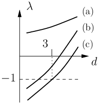
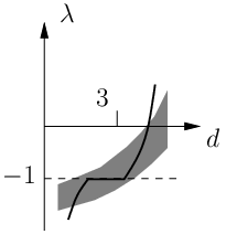
The previous arguments are compelling but not mathematically rigorous. In particular, assuming that the theory can be properly defined in noninteger dimensions, which is standard but not obvious, it is hard to control the analytic structure of the critical exponents in $d$. In the next section, we give a proof in the physically important case of the Ising model in $d=3$ which does not rely on such arguments.

We concentrate here on the Ising universality class and show that, in this case, the smallest eigenvalue $D_{V}$ associated with an integrated vector perturbation is larger than $-1$ for $d<4$. Using our necessary condition, this proves that, for the Ising universality class, the critical regime is conformally invariant.

For simplicity, we consider a lattice version of the Ginzburg-Landau model whose dynamics is described by the hamiltonian (or action)

where the index $i$ labels the lattice sites, the $\varphi(i)$ take values in the real domain and $U(\varphi)$ is an even function that diverges for $|\varphi|\to\infty$. We choose here a hypercubic lattice with lattice spacing $a$. The original Ising model can be recovered by considering a potential $U(\varphi)$ strongly peaked around $\varphi=\pm 1$ but the Ginzburg-Landau model which is in the Ising universality class for a generic potential is more convenient for what follows.

The use of Ginzburg-Landau model has another advantage. In the case of a quartic potential,

and for $d<4$, the model is super-renormalizable. Its ultraviolet behaviour is therefore controlled by a Gaussian fixed-point. In this case, the existence of a controlled scaling limit seems to be under control even if, to the best of our knowledge, there is no mathematical proof of its existence [39]. To compare different models in the Ising universality class we assume below that this scaling limit does exist in the following precise sense. Let us consider two local operators $\mathcal{O}_{1}(i,a)$ and $\mathcal{O}_{2}(i,a)$. Let us also introduce (i) a smooth interpolating field $\phi^{\rm interp}(x)$ with $x\in\mathbb{R}^{d}$ that coincides on the lattice points with $\phi(i)$ and (ii) two interpolating operators ${\cal O}_{1,2}^{\rm interp}(x,a)$ defined by: ${\cal O}_{i}^{\rm interp}={\cal O}_{i}(\phi^{\rm interp})$. Of course the construction of these interpolating operators is not unique. We now consider the particular case where ${\cal O}_{1}$ and ${\cal O}_{2}$ are such that ${\cal O}_{1}^{\rm interp}\to{\cal O}_{2}^{\rm interp}$ when $a\to 0$. (We notice that this limit is independent of the choice of interpolation used to define $\phi^{\rm interp}$). Our assumption, that we call for short “scaling limit”, is that there exists a multiplicative factor $Z_{\mathcal{O}}(a)$ depending on the lattice spacing such that the correlation functions of the operators $\mathcal{O}_{1}(x,a)$ and $Z_{\mathcal{O}}(a)\mathcal{O}_{2}(x,a)$ are the same for distances much larger than $a$:

where $\{\mathcal{O}_{3},\dots,\mathcal{O}_{n}\}$ are arbitrary local operators and where the equivalence occurs for $a\ll\min\{|y_{3}-x|,\dots,|y_{n}-x|\}$. This hypothesis is a pre-requisite of all Monte Carlo simulations, and is, of course, satisfied to all orders of perturbation theory in any renormalizable theory. We assume here that it is also valid nonperturbatively.

Our strategy is to study correlation functions of local vector operators $\mathcal{V}_{\mu}(x)$ and use their critical behavior to find a bound on the scaling dimension of the integrated operator $V_{\mu}=a^{d}\sum_{i}\mathcal{V}_{\mu}(i)$. We rightaway mention two difficulties.

First, there are local vector operators that are total derivatives and which are therefore not associated with an integrated one. As discussed before, the vector operator $\partial_{\mu}(\varphi^{2})$ is such an operator. Note that its scaling dimension near $d=4$ is lower than that of the vector operators which are not total derivatives (such as $\partial_{\mu}(\varphi)^{2}(\partial_{\nu}\varphi)^{2}$).

Second, operators with the same quantum numbers typically mix together in the calculation of correlation functions. As a consequence, the critical behavior of a two-point function of some vector operator is governed by the lowest scaling dimension of the class of operators with which it mixes. To be more precise, let us call $\mathcal{V}_{\mu}^{(n)}$ the local vector eigenoperator of scaling transformations with scaling dimension $D_{\mathcal{V}}^{(n)}$ (ordered such that $D_{\mathcal{V}}^{(0)}\leq D_{\mathcal{V}}^{(1)}\leq\cdots$). The associated two-point correlation function behaves, in the critical regime, as:

where the subscript c indicates connected correlation functions, defined as:

and where an appropriate normalization has been chosen. In $d=4$, the eigenproblem can be solved and the scaling dimensions are the canonical dimensions. In particular, the eigenoperators with lowest scaling dimensions are:

where $\partial_{\mu}$ is a lattice discretization of the partial derivative. (Note that the first three operators are total derivatives.) In dimension $d<4$, although we do not know the explicit form of the eigenoperators, we can, in principle, decompose any vector operator on the basis $\{{\mathcal{V}}_{\mu}^{(n)}\}$ and generically, there is a nonvanishing overlap with each of the eigenoperators:

As a consequence, the critical regime of the two-point correlation function is dominated by the smallest critical dimension

We stress that the list of quantum numbers must include those associated with lattice isometries. For example, we require scalar (respectively vector) operators defined on the lattice to be even (respectively odd) under parity transformations.

The proof is organized as follows. Using Lebowitz inequalities [40, 41], we derive a lower bound for $D_{\cal V}^{(0)}$ from which follows a lower bound for the scaling dimension of the integrated vector operators. The proof that the scaling dimension $D_{V}$ of any integrated vector operator is different from $-1$ for $d\leq 4$ is then a direct consequence of this bound.

As a first step, we derive a bound for the correlation function $\langle\varphi^{2}(x)\varphi^{2}(y)\rangle_{\text{c}}$. We use here the Lebowitz inequalities [40] which state that, considering two decoupled copies of the ferromagnetic system (that we note $\varphi$ and $\varphi^{\prime}$), both described by the action (22), and considering two sets $A$ and $B$ of lattice points,

In particular, this implies that:

Expanding the binomials, we readily obtain the following identity:

where we have used the fact that the average of an odd number of fields vanishes for temperatures higher than (or equal to) the critical temperature. This implies that the connected correlation function $\langle\varphi^{2}(x)\varphi^{2}(y)\rangle_{\text{c}}$ cannot decrease more slowly than the square of the propagator at long distances. This inequality can be generalized to arbitrary even powers of the fields:

where $C$ is a positive constant (that depends on $m$ and $n$) as shown in the Appendix A.

In the critical regime, scale invariance implies that connected two-point correlation functions behave as power-laws. In particular:

with $A$ a positive constant (see, for example [14]). The inequality (37) implies that $\aleph_{n}\geq d-2+\eta$. We can then deduce the asymptotic behavior of the matrix of second derivatives of this correlation function:

where $B$ and $C$ are some constants.

We now consider two local vector operators that are the product of one power of $\partial_{\mu}\varphi(x)$ and an odd (finite) number of fields evaluated at points in a finite neighborhood of $x$:

where $e_{i}^{(1)}$ and $e_{i}^{(2)}$ are some constant lattice vectors⁴⁴ 4 Since $\Sigma_{\mu}$, defined in Eq. (14), is odd under parity, it is important in what follows to consider only vector operators that are also odd. This is the reason why the sum over $s$ is necessary in the definitions (40) and (41).. The operators $W_{\mu}^{(1)}(x)$ and $W_{\mu}^{(2)}(x)$ are, up to a multiplicative constant, other discretizations of, respectively, the operator $\partial^{x}_{\mu}(\varphi^{m}(x))$ and $\partial^{x}_{\mu}(\varphi^{n}(x))$. According to the assumption of the existence of the scaling limit, Eq. (24), the connected correlation function $\langle\mathcal{W}_{\mu}^{(1)}(x)\mathcal{W}_{\nu}^{(2)}(y)\rangle_{\text{c}}$ has the same asymptotic behavior as in Eq. (39) up to a multiplicative factor depending on the lattice spacing. Indeed, when $|x-y|$ is much larger than the lattice spacing $a$, the vectors $e_{i}^{(1)}$ and $e_{i}^{(2)}$ can be neglected in (40) and (41) and the local operators $\mathcal{W}_{\mu}^{(1)}$ and $\mathcal{W}_{\mu}^{(2)}$ are then proportional to $\partial_{\mu}(\varphi^{m})$ and $\partial_{\nu}(\varphi^{n})$ respectively as explained before.

Now, any local vector operator ${\mathcal{V}}_{\mu}$ on the lattice is a linear combination of vector operators of the form (40). For instance, a discretization of the operator $\partial_{\mu}(\phi^{2})(\partial_{\nu}\phi)^{2}$ is given by:

where the sum runs over all the nearest neighbors of $x$.

Using the triangular inequality, we conclude that:

where $Z_{\mu\nu}$ is a positive constant. Using Eq. (32) this implies that, for all $n$:

We conclude that the scaling dimension $D_{V}=D_{\mathcal{V}}-d$ of any integrated vector operator is not smaller than $-1+\eta$.⁵⁵ 5 This bound also applies for correlation functions of more general operators. Using the unitarity of the Minkowskian $\phi^{4}$ theory, one can prove that $\eta\geq 0$ [42] for the Ising universality class. Moreover, an interacting massless theory such as the critical Ising model for $d<4$, has a non-zero $\eta$ [43]. As a consequence, our necessary condition is fulfilled and we conclude that scale invariance implies conformal invariance for the Ising universality class for all $d\leq 4$.

Let us now point out some directions of research for the future. It is clear that the condition of conformal invariance (14) can be straightforwardly extended to other theories (involving scalar, fermionic or vector fields) and it would be interesting to conclude on the fate of conformal invariance in this wider class of models. In these systems, it is much more difficult to find rigorous bounds on correlation functions (that would generalize the Lebowitz inequalities). It would then prove useful to approach the problem by computing the scaling behavior of vector operators by Monte-Carlo simulations.

Another promising line of investigation consists in making use of the conformal invariance in the Wilson framework to perform actual calculations of universal quantities. On the one hand, and in the best case, this would lead to closed and numerically tractable equations for the critical exponents. On the other hand, the approximation schemes currently used for solving the Wilson RG flow equation being incompatible with exact conformal invariance, we can expect that constraining them to be conformally invariant at the fixed point would improve their accuracy.

Notice finally that, at first sight, our approach could seem similar to the one based on the energy-momentum tensor and on the analysis of the virial current. This is not the case although there is perhaps a relationship between the two. $\Sigma^{\mu}_{k}$ is a functional of $\phi$ and not of $\varphi$; it is built from $\Gamma_{k}$ and not from $S$; what matters is that its density vanishes up to a surface term and not that it is conserved. Moreover, as we already explained, we only deal with a regularized theory which enables us to consider only the analytic candidates for $\tilde{\Sigma}^{\mu*}$ contrary to what should be done in a nonregularized theory. In any case, a clarification of the relation between the two approaches would be welcome. In this respect, our proof of the non-existence of local vector operator of scaling dimension $d-1$ (conserved or not) might be of interest also when applied to a hypothetical conserved virial current.

References

- [1] J. M. Maldacena, Int. J. Theor. Phys. 38, 1113 (1999) [Adv. Theor. Math. Phys. 2, 231 (1998)].
- [2] S. El-Showk, M. F. Paulos, D. Poland, S. Rychkov, D. Simmons-Duffin and A. Vichi, Phys. Rev. D 86, 025022 (2012).
- [3] F. Gliozzi and A. Rago, J. High Energy Phys. 10 (2014) 042.
- [4] S. El-Showk, M. F. Paulos, D. Poland, S. Rychkov, D. Simmons-Duffin and A. Vichi, J. Stat. Phys. 157, 869 (2014).
- [5] F. Kos, D. Poland and D. Simmons-Duffin, J. High Energy Phys. 06 (2014) 091.
- [6] S. El-Showk, M. Paulos, D. Poland, S. Rychkov, D. Simmons-Duffin and A. Vichi, Phys. Rev. Lett. 112, 141601 (2014).
- [7] Y. Nakayama and T. Ohtsuki, Phys. Rev. D 91, 021901(R) (2015).
- [8] M. S. Virasoro, Phys. Rev. D 1, 2933 (1970).
- [9] A. M. Polyakov, JETP Lett. 12, 381 (1970) [Pisma Zh. Eksp. Teor. Fiz. 12, 538 (1970)].
- [10] A. A. Migdal, Phys. Lett. B 37, 386 (1971).
- [11] A. A. Belavin, A. M. Polyakov and A. B. Zamolodchikov, Nucl. Phys. B 241, 333 (1984).
- [12] A. B. Zamolodchikov, JETP Lett. 43, 730 (1986) [Pisma Zh. Eksp. Teor. Fiz. 43, 565 (1986)].
- [13] J. Polchinski, Nucl. Phys. B 303, 226 (1988).
- [14] P. Di Francesco, P. Mathieu and D. Sénéchal, Conformal field theory (Springer, New York, 1997), p. 890.
- [15] K. G. Wilson and J. B. Kogut, Phys. Rept. 12, 75 (1974).
- [16] I. Jack and H. Osborn, Nucl. Phys. B 343, 647 (1990).
- [17] M. A. Luty, J. Polchinski and R. Rattazzi, J. High Energy Phys. 01 (2013) 152.
- [18] A. Dymarsky, Z. Komargodski, A. Schwimmer and S. Theisen, arXiv:1309.2921 [hep-th].
- [19] A. Dymarsky, K. Farnsworth, Z. Komargodski, M. A. Luty and V. Prilepina, arXiv:1402.6322 [hep-th].
- [20] L. Schafer, J. Phys. A 9, 377 (1976).
- [21] O. J. Rosten, arXiv:1411.2603 [hep-th].
- [22] J. Polchinski, Nucl. Phys. B 231, 269 (1984).
- [23] C. Wetterich, Phys. Lett. B 301, 90 (1993).
- [24] U. Ellwanger, Z. Phys. C 58, 619 (1993).
- [25] T. R. Morris, Int. J. Mod. Phys. A 9, 2411 (1994).
- [26] J. Berges, N. Tetradis and C. Wetterich, Phys.Rept. 363, 223 (2002).
- [27] T. Machado and N. Dupuis, Phys. Rev. E 82, 041128 (2010).
- [28] C. Becchi, hep-th/9607188.
- [29] U. Ellwanger, Phys. Lett. B 335, 364 (1994).
- [30] J. M. Pawlowski, Annals Phys. (N.Y.) 322, 2831 (2007).
- [31] J. M. Kosterlitz and D. J. Thouless, J. Phys. C 6, 1181 (1973).
- [32] A. B. Zamolodchikov, Sov. J. Nucl. Phys. 44, 529 (1986) [Yad. Fiz. 44, 821 (1986)].
- [33] T. R. Morris, Phys. Lett. B 345, 139 (1995)
- [34] T. R. Morris and M. D. Turner, Nucl. Phys. B 509, 637 (1998).
- [35] T. R. Morris, Phys. Rev. Lett. 77, 1658 (1996).
- [36] T. R. Morris, Nucl. Phys. B 495, 477 (1997).
- [37] V. Riva and J. L. Cardy, Phys. Lett. B 622, 339 (2005).
- [38] S. El-Showk, Y. Nakayama and S. Rychkov, Nucl. Phys. B 848, 578 (2011)
- [39] A. Abdesselam and V. Rivasseau, private communication.
- [40] J.L. Lebowitz, Commun. Math. Phys. 35, 87 (1974).
- [41] J. Glimm and A. Jaffe, Quantum Physics: A Functional Integral Point of View, 2nd ed. (Springer-Verlag, New York, 1987).
- [42] J. Zinn-Justin, Int. Ser. Monogr. Phys. 113, 1 (2002).
- [43] K. Pohlmeyer, Commun. Math. Phys. 12, 204 (1969).
- [44] R. B. Griffiths, J. Math. Phys. 8, 478 (1967); 8, 484 (1967).
- [45] D. G. Kelly and S. Sherman, J. Math. Phys. 9, 466 (1968).