Global hybrids from the semiclassical atom theory satisfying the local density linear response
Abstract
We propose global hybrid approximations of the exchange-correlation (XC) energy functional which reproduce well the modified fourth-order gradient expansion of the exchange energy in the semiclassical limit of many-electron neutral atoms and recover the full local density approximation (LDA) linear response. These XC functionals represent the hybrid versions of the APBE functional [Phys. Rev. Lett. 106, 186406, (2011)] yet employing an additional correlation functional which uses the localization concept of the correlation energy density to improve the compatibility with the Hartree-Fock exchange as well as the coupling-constant-resolved XC potential energy. Broad energetical and structural testings, including thermochemistry and geometry, transition metal complexes, non-covalent interactions, gold clusters and small gold-molecule interfaces, as well as an analysis of the hybrid parameters, show that our construction is quite robust. In particular, our testing shows that the resulting hybrid, including 20% of Hartree-Fock exchange and named hAPBE, performs remarkably well for a broad palette of systems and properties, being generally better than popular hybrids (PBE0 and B3LYP). Semi-empirical dispersion corrections are also provided.
I Introduction
Density functional theory (DFT) [1, 2] is nowadays one of the most popular methods in electronic structure calculations. DFT is an exact theory, but its practical implementation requires an approximation for the so-called exchange-correlation (XC) energy functional, which describes the quantum effects of the electron-electron interaction. Many approximated expressions, having different levels of complexity/sophistication, exist for this functional [3, 4]. They can be roughly classified in two broad classes: i) local and semilocal functionals, using as input information the electron density, its derivatives, and the kinetic energy density; ii) fully non-local functionals, which additionally use as input non-local quantities computed from the Kohn-Sham orbitals (e.g. exact exchange). The former ones, which include local density, generalized gradient and meta generalized gradient approximations (LDA, GGAs, and meta-GGAs, respectively), are fast and sufficiently accurate for many purposes [5, 6, 7, 8, 9, 10, 11, 12, 13, 14, 15, 16, 17, 18, 19, 20], but fail for a number of important properties such as density distributions or barriers heights [21, 22, 23, 24, 25]. The second ones, which include global, range-separated, local and double hybrid functionals [26, 27, 28, 29, 30, 31, 32, 33, 34, 35, 36, 37, 38, 39, 40, 41, 42, 43, 44, 45, 46, 47, 48, 49, 50, 51, 52, 53, 54, 22, 55, 56, 57], improve considerably the results, but they are much more computer-time demanding, in particular when local or double hybrids are used.
Among functionals of the second class, global hybrids provide the best compromise between accuracy and efficiency. They are characterized by an exchange energy contribution which is a mixing of exact exchange and a local or semilocal contribution. In global hybrids, a fraction of Hartree-Fock exchange energy is directly combined with the complementary fraction of an exchange energy functional.
The great majority of the hybrid functionals are parameterized: the constant determining the relative weight of the exact and semilocal exchange and (in most cases) some other parameters are fixed by fitting some training datasets. Furthermore, fitted parameters can also be contained in the semilocal functional used in the hybrid construction. A well-known example of parameterized hybrid functional is B3LYP [58, 59, 60, 61].
On the other hand, there are few examples of non-parameterized hybrid functionals. In the case of global hybrids (the one of interest in the present paper) the parameter determining the ratio between exact and semilocal exchange can be chosen by theoretical arguments [33, 36]. Then, constructing the hybrid on the basis of a non-parameterized semilocal functional, one obtains a parameter-free (or non-empirical) hybrid functional. PBE0 [33, 34, 35] and, more recently, PBE0-1/3 [36, 37] have been obtained in such a way. Extensive calculations of molecular properties have shown that non-parameterized hybrids are not only more satisfactory than the parameterized ones from the theoretical point of view, but they are also competitive in terms of accuracy, in particular when systems or properties that do not belong to the training sets of the parameterized hybrids are considered.
In the present paper, we construct and test parameter-free hybrids based on the APBE GGA functional [62]. This is a non-parameterized GGA constructed from the semiclassical atom model and has shown high accuracy for a wide range of molecular properties [63]. Moreover, in our development of the hybrid form, we deviate from the conventional scheme and explore the possibility of combining the exact exchange with an additional correlation functional. This procedure is motivated, within the adiabatic connection scheme [26, 33, 36], by the need to correct the correlation contribution associated to the exact exchange fraction, when the coupling constant is approaching one. A similar motivation stands at the base of double hybrids, where the correlation is however partly treated at the MP2 level.
The paper is organized as follows: in the next section we present the theory at the base of our construction of the hybrid functionals and discuss it in the context of the adiabatic connection. A possible spin-dependent correction for the correlation is discussed as well. In the following section we show the performance of our hybrid functionals in comparison with other relevant ones, using a broad set of molecular tests. The results are discussed also in terms of the role of the parameters defining the hybrids. Finally, we provide a brief study on the use of a semiempirical dispersion correction in conjuction with the functionals presented in this work.
II Theory
II.1 Construction of the hybrid functional
According to the adiabatic connection the exchange-correlation (XC) functional is given by the coupling-constant integration formula
| (1) |
where is an appropriate coupling-constant-resolved XC potential energy. One popular choice for to derive global hybrid functional is the ansatz proposed by Perdew, Ernzerhof, and Burke [33]:
| (2) |
where DFA stands for some local or semilocal density functional approximation and is the Hartree-Fock exchange computed with Kohn-Sham orbitals. This formula correctly reverts to exact-exchange-only when (i.e. for the non-interacting system) and assumes that is well approximated by DFA[33, 64]. We recall [33] that , where , with being the uniform scaled spin-densities. Thus, is a density functional approximation for the correlation potential ( and ), and Eq. (2) describes, at small non-vanishing values of the coupling constant , a mixing of the DFT exchange with the exact exchange, but with full DFT correlation as given by DFA. Using Eq. (2) in Eq. (1) we have:
| (3) |
which shows that always the same is used in combination with different value of . This situation appears not to be optimal, since in general the DFA correlation contribution is designed to work well together with its DFA exchange counterpart but not with the HF exchange. Thus, it may be appropriate to generalize Eq. (3). Hence, we propose the generalized ansatz
| (4) | |||||
so that after integration we obtain
| (5) | |||||
where the integer parameter controls how the correlation functionals and are mixed. We note that Eq. (4) is exact at , as Eq. (2), while at we have , differently from Eq. (2). As shown in the Appendix, Eq. (4) can yield an improved coupling-constant-resolved XC potential for atoms. In this work, we will choose for DFA1 the APBE GGA functional [62], which is one of the most accurate non-empirical GGAs with broad applicability [62, 63]. For DFA2, we select the PBEloc correlation functional [66], which has been proved to work quite well together with the Hartree-Fock exchange, even if other possibilities could also be considered [67, 68, 6]. Note that Eq. (5) resembles the general expression of two-parameter double hybrid functionals [65], if is replaced by the MP2 correlation energy and the constraint on and to be integer numbers is relaxed.
In order to use only one parameter, we need a relation between and . We note that the APBE functional was constructed in such a way that it recovers the accurate LDA linear response behavior [69, 70]. Similarly the PBEloc functional was designed to respect the same property with respect to exact exchange. Thus, it appears a natural choice to force the full hybrid functional to respect the accurate LDA linear response behavior. To this end we need to put in Eq. (5). The final formula for the hybrid XC functional is therefore
| (6) |
Equation (6) shows that the resulting XC energy is just a linear mixing of the original APBE XC functional with the functional: thus a good accuracy can be expected only if PBEloc works well in combination with HF, as it is indeed the case[66].
We recall that the relevance of the LDA linear response behavior has been already discussed for the semilocal level of the theory [71, 62, 63, 72], and even for hybrid functionals [73]. However, in Ref. 73 only the linear response behavior of the semilocal fraction of the functional is considered. We will discuss this item even further in the final part of this paper (Section IV.1), where the condition will be released.
Moreover, we recall that was constructed from the semiclassical theory of large neutral atoms, and recovers the modified second-order gradient expansion (MGE2) [62]. It was proved that MGE2 can reproduce well the fourth-order gradient expansion (GE4) [62, 74, 75]. Thus, because already recovers the GE4, the whole exchange part of the hybrid given in Eq. (6) reproduces to a good accuracy the GE4 in the slowly-varying atomic density limit. This feature however, can be met exactly only at the meta-GGA hybrid level (e.g. the TPSSh hybrid [76]).
The value of the remaining parameter can be strongly circumscribed by theoretical considerations based on perturbation theory [33, 36] but not univocally fixed. The more convenient choice depends on the semilocal functional(s) used in the hybrid construction and is ultimately determined by the result accuracy. In this work we consider or 5. The corresponding functionals are assessed in next sections. These functionals have the same exact exchange content as the popular PBE0 [33, 34, 35] and B3LYP [58, 59, 60, 61] hybrid functionals, respectively. We note that additional values of can be considered. In particular, the value , which can also be obtained from perturbation theory [36], was shown to yield good results for organic chemistry [37] and excited states, in particular when charge transfer [77] and Rydberg transitions [78] are considered. However, such higher fractions of exact exchange do not provide a global result improvement for the datasets considered in the present paper, thus they will not be discussed any longer in this work.
II.2 Spin-dependent correction for the PBEloc functional
The good compatibility of the PBEloc functional with the Hartree-Fock exchange is based on a localization paradigm of the correlation energy density [66, 8, 10]. In Ref. 67 it has been shown that this localization, and consequently the compatibility with exact exchange, can be further enhanced, preserving the exact properties of PBEloc, by a slight modification of the original correlation functional to
| (7) |
where is the electron density, is the PBEloc correlation energy per particle, and
| (8) |
is a spin-dependent correction factor with being a reduced gradient suitable for density variations in valence and bonding regions [67], , and being the relative spin polarization.

To fix the parameters and in Eq. (8) we used the uniformly spin-polarized Gaussian (G) and hydrogenic (H) one-electron density models and , with and respectively, requiring an improved spin-behavior for . We recall that the ideal spin-behavior for these model systems is [67]
| (9) |
with . We finally obtain and . As shown in Table 1 the so obtained correlation zvPBEloc functional displays an improved compatibility with Hartree-Fock exchange, with respect to the original PBEloc, for tests on small molecules where dynamical correlation is relevant (see Refs. 67, 96 for more details). Moreover, Fig. 1 shows that zvPBEloc provides a better behavior with respect to PBEloc, yet preserving the PBEloc shape, for both H and G densities.
| Test set | PBE | LYP | PBEloc | zvPBEloc |
|---|---|---|---|---|
| AE6 | 31.9 | 38.2 | 24.0 | 20.8 |
| BH6 | 5.6 | 5.3 | 4.4 | 4.6 |
| K9 | 5.7 | 6.0 | 4.7 | 4.2 |
To take advantage of the improved features of the zvPBEloc functional we will thus consider also global hybrids of the form
| (10) |
III Computational details
To assess the performance of the functionals we performed calculations on a large test set (overall more than 500 systems and various energetical and structural ground-state properties), which was divided into five main groups:
- •
Thermochemistry. This group considers the atomization energies of small molecules (AE6 [82, 83] and W4 [55, 85, 86]) and molecules with non-single-reference character (W4-MR [55]), proton affinities (PA12 [87, 88, 89, 85, 86]) and ionization potentials (G21IP [90, 85, 86]), different barrier heights (BH76 [91, 92, 85, 86]), reaction energies (BH76RC [91, 92, 85, 86] and OMRE [23]), and both barrier heights and reaction energies (K9 [84, 83]).
- •
- •
Transition metals. This group of tests includes atomization energies of small transition metal complexes (TM10AE [95, 96]) and gold clusters (AUnAE [96, 97], reaction energies of transition metal complexes (TMRE [23, 95]), and bond lengths of transition metal complexes (TMBL [96, 98]) and gold clusters (AuBL6 [23, 97]). Note that here for the TM10AE test have been used tighter convergence criteria than in previous publications [96, 8].
- •
Non-covalent interactions. This group considers interaction energies of hydrogen-bond (HB6 [99]), dipole-dipole (DI6 [99]), charge-transfer (CT7 [99]), and --stacking (pp5 [99]) complexes. In addition, interaction energies of dihydrogen-bond complexes (DHB23 [100]) and of complexes with various character (S22 [101, 102]) are taken into account.
- •
Other properties. This group considers a miscellaneous of other properties and systems including isomerization energies of large organic molecules (ISOL6 [103]), difficult cases for DFT (DC9/12 [104]), small gold-organic interfaces (SI12 [23]), dipole moments of organic molecules (DM25 [23]), and atomic energies (AE17 [31]).
All tests were carried out for the functionals defined by Eqs. (6) and (10) with 4 or 5. For completeness also the hybrid functional named APBE0 and defined as was considered (this is in practice obtained from Eq. (6) changing with and setting ).
For comparison we performed calculations using several other GGA and hybrid functionals: the PBE [71] and APBE [62] GGA functionals, as well as the popular hybrid XC functionals PBE0 [33, 34, 35] and B3LYP [58, 59, 60, 61]. Finally, we considered also the PBEmol0 hybrid functional [73] which was constructed to restore the LDA linear response in the semilocal part of the functional by scaling the second-order coefficient in the correlation part. Note that, because the GGA functional PBEmol [73] is very similar to APBE, the PBEmol0 hybrid functional practically differs from Eq. (6) only for the fact that in the former the LDA linear response condition is enforced only in the semilocal part, while in the later it is extended to the whole functionals (thanks to the inclusion of the PBEloc correction).
All calculations have been performed with the TURBOMOLE program package [105] using a def2-TZVPP basis set [106, 107]. The choice of the basis set was motivated by the need to find a best compromise between accuracy and computational cost, so that our results can be directly compared to practical applications. We note also that because the same basis set is used for all the functionals a fair assessment of relative performances is possible.
To evaluate the performance of the different approaches we computed, for each group of tests outlined above, the average MAE relative to PBE0, which is assumed as a reference. Hence, we considered
| (11) |
where the sum runs over all the tests within a group and MAE is the MAE of PBE0 for the -th test. The RMAE indicates whether any method is better (RMAE1) or worse (RMAE1) than PBE0. The RMAE provides a fair global assessment of all the results, however it may tend to overweight tests where both MAEi and MAE are small and to underweight the results of tests where both methods yield quite poor results. For this reason, in addition to the RMAE, we considered also the weighted MAE
| (12) | |||||
where is the average of the MAEs of all hybrid methods for test . Equation (12) shows that in the WMAE the quantities composing the RMAE are averaged with weights , which indicate the relative performance of PBE0 (assumed as a reference) with respect to what may be expected from hybrid approaches. Hence, negative WMAEs denote methods outperforming PBE0, while positive values denote methods performing worse than PBE0.
IV Results
| Test | GGA | Hybrid | Hybrid | |||||||||
|---|---|---|---|---|---|---|---|---|---|---|---|---|
| PBE | APBE | B3LYP | Eq. (6) | Eq. (10) | PBE0 | APBE0 | PBEmol0 | Eq. (6) | Eq. (10) | |||
| Thermochemistry (kcal/mol) | ||||||||||||
| atomization energy (AE6) | 13.4 | 7.8 | 5.5 | 5.8 | ∗4.2 | 6.3 | 9.5 | 7.3 | 6.8 | 4.8 | ||
| atomization energy (W4) | 10.7 | 8.5 | 5.8 | 6.4 | ∗6.0 | 6.0 | 8.7 | 7.6 | 7.3 | 6.4 | ||
| static correlation (W4-MR) | 21.8 | 17.4 | 8.4 | ∗5.9 | ∗5.9 | 7.1 | 10.5 | 11.2 | 9.1 | 7.2 | ||
| proton affinities (PA12) | 2.2 | 2.8 | 2.3 | ∗3.1 | ∗3.1 | 2.8 | 3.4 | 3.5 | 3.3 | 3.3 | ||
| ionization pot. (G21IP) | 3.9 | 4.0 | 3.8 | ∗4.0 | ∗4.0 | 4.1 | 4.2 | 4.6 | 4.2 | 4.2 | ||
| barrier heights (BH76) | 9.8 | 9.0 | 5.0 | 5.0 | 5.0 | 4.5 | 3.9 | 4.0 | ∗4.2 | ∗4.2 | ||
| reaction energies (BH76RC) | 4.4 | 3.8 | 2.6 | 2.8 | 2.9 | 2.7 | 2.5 | 2.4 | ∗2.6 | 2.7 | ||
| reaction energies (OMRE) | 6.7 | 7.1 | 4.6 | 6.5 | ∗6.4 | 9.1 | 7.1 | 6.0 | 8.1 | 7.9 | ||
| kinetics (K9) | 7.5 | 6.6 | 3.8 | 4.2 | 4.2 | 3.9 | 3.3 | 3.1 | ∗3.7 | ∗3.7 | ||
| RMAE | 1.71 | 1.46 | 0.96 | 1.00 | ∗0.96 | 1.00 | 1.15 | 1.09 | 1.07 | 0.99 | ||
| WMAE(%) | +66 | +42 | -6 | -1 | ∗-4 | 0 | +11 | +6 | +6 | -2 | ||
| Organic molecules’ geometry (mÅ, and cm-1) | ||||||||||||
| H bond lengths (MGHBL9) | 11.4 | 10.2 | 3.0 | ∗1.4 | ∗1.4 | 2.3 | 1.5 | 1.0 | 1.5 | 1.5 | ||
| non-H bond lengths (MGNHBL11) | 7.6 | 9.2 | 7.2 | ∗7.3 | ∗7.3 | 9.8 | 8.8 | 8.7 | 10.7 | 10.6 | ||
| open-shell molecules (BL9) | 15.0 | 14.7 | 11.9 | ∗11.6 | ∗11.6 | 12.7 | 12.2 | 12.3 | 12.5 | 12.5 | ||
| vibrations (F38) | 58.4 | 55.0 | 37.1 | ∗44.2 | ∗44.2 | 53.3 | 52.0 | 52.1 | 58.3 | 58.3 | ||
| RMAE | 2.00 | 1.88 | 0.91 | ∗0.77 | ∗0.77 | 1.00 | 0.86 | 0.82 | 0.96 | 0.96 | ||
| WMAE(%) | +135 | +119 | -7 | ∗-28 | ∗-28 | 0 | -17 | -23 | -7 | -7 | ||
| Transition metal complexes (kcal/mol [for AUnAE kcal/(molatoms)] and mÅ) | ||||||||||||
| atomization energy (TM10AE) | 13.0 | 11.1 | 13.4 | 12.1 | ∗11.0 | 14.4 | 15.8 | 14.0 | 14.1 | 11.4 | ||
| reaction energies (TMRE) | 3.7 | 3.1 | 10.6 | 9.6 | ∗8.4 | 9.0 | 9.5 | 9.5 | 11.5 | 9.2 | ||
| gold clusters atomiz. (AUnAE) | 0.60 | 1.8 | 5.9 | ∗3.8 | ∗3.8 | 4.0 | 5.1 | 5.0 | 4.3 | 4.3 | ||
| bond lengths (TMBL) | 13.5 | 13.0 | 18.5 | ∗18.3 | ∗18.3 | 21.2 | 20.6 | 20.5 | 21.8 | 21.8 | ||
| gold clusters bonds (AuBL6) | 56.5 | 58.7 | 94.2 | 36.6 | 36.5 | 41.9 | 56.0 | 58.9 | 32.5 | ∗32.3 | ||
| RMAE | 0.69 | 0.72 | 1.34 | 0.92 | ∗0.88 | 1.00 | 1.15 | 1.13 | 1.03 | 0.94 | ||
| WMAE(%) | -30 | -28 | +29 | -8 | ∗-12 | 0 | +13 | +11 | +3 | -6 | ||
| Non-covalent interactions (kcal/mol) | ||||||||||||
| hydrogen bonds (HB6) | 0.38 | 0.32 | 0.55 | ∗0.36 | ∗0.36 | 0.52 | 0.36 | 0.45 | 0.38 | 0.38 | ||
| dipole-dipole (DI6) | 0.38 | 0.39 | 0.88 | ∗0.38 | ∗0.38 | 0.36 | 0.38 | 0.32 | ∗0.38 | ∗0.38 | ||
| dihydrogen bonds (DHB23) | 0.98 | 0.76 | 0.34 | ∗0.66 | ∗0.66 | 0.75 | 0.56 | 0.79 | ∗0.66 | ∗0.66 | ||
| charge-transfer (CT7) | 2.7 | 2.4 | 0.79 | 1.3 | 1.3 | 1.3 | 1.0 | 1.2 | ∗1.2 | ∗1.2 | ||
| - stacking (pp5) | 2.1 | 2.2 | 3.2 | ∗2.2 | ∗2.2 | 2.1 | 2.2 | 2.0 | ∗2.2 | ∗2.2 | ||
| various non-covalent (S22) | 2.3 | 2.7 | 3.5 | ∗2.4 | ∗2.4 | 2.2 | 2.4 | 2.2 | ∗2.4 | ∗2.4 | ||
| RMAE | 1.21 | 1.13 | 1.27 | 0.97 | 0.97 | 1.00 | 0.91 | 0.95 | ∗0.95 | ∗0.95 | ||
| WMAE(%) | +23 | +15 | +22 | -5 | -5 | 0 | ∗-12 | -6 | ∗-7 | ∗-7 | ||
| Other (kcal/mol; Debye/10 for DM25) | ||||||||||||
| isomerization (ISOL6) | 2.2 | 2.4 | 2.7 | ∗1.4 | ∗1.4 | 1.5 | 1.4 | 1.4 | ∗1.4 | ∗1.4 | ||
| difficult cases (DC9.12) | 40.8 | 29.4 | 25.0 | 19.7 | 19.6 | 17.7 | 22.9 | 20.2 | 18.2 | ∗17.9 | ||
| small interfaces (SI12) | 3.7 | 5.9 | 11.0 | ∗7.0 | 7.1 | 7.2 | 8.9 | 9.3 | 7.8 | 7.9 | ||
| dipole moments (DM25) | 3.6 | 3.6 | 2.9 | 2.7 | 2.7 | 2.7 | 2.7 | 2.7 | ∗2.6 | ∗2.6 | ||
| atomic energies (AE17) | 51.6 | 22.2 | 7.6 | 16.9 | 16.6 | 42.2 | 10.2 | 54.5 | 15.7 | ∗15.3 | ||
| RMAE | 1.36 | 1.19 | 1.20 | 0.88 | 0.88 | 1.00 | 0.94 | 1.13 | 0.88 | ∗0.87 | ||
| WMAE(%) | +38 | +9 | +2 | -22 | -23 | 0 | -21 | +17 | ∗-24 | ∗-24 | ||
| Global RMAE | 1.41 | 1.27 | 1.12 | 0.92 | ∗0.90 | 1.00 | 1.02 | 1.03 | 0.99 | 0.94 | ||
| Global WMAE(%) | +44 | +28 | +5 | -11 | ∗-13 | 0 | -4 | +2 | -5 | -9 | ||
Table 2 reports the mean absolute error (MAE) for each test as obtained from the different functionals. We see that the best overall performance is given by the hybrid functional defined by Eq. (10) with (named hAPBE hereafter), which yields a global RMAE of 0.90 and a global WMAE of -13%. Notably it is also the best non-fitted hybrid functional for three out of five groups of tests that we considered (thermochemistry, organic molecules’ geometry, and transition metals) and it is very close to the best results for the remaining two groups. Moreover, hAPBE provides results more accurate than the average of the considered hybrids in 23 over 28 cases. For thermochemistry the hAPBE functional yields performance very close to the B3LYP functional (RMAE is the same; WMAE is only 2% better in B3LYP) which was fitted on some of these properties. However B3LYP shows, several limitations for other problems, especially those related to transition metals and clusters, being below the average performance in most tests not connected to thermochemistry. These limitations may possibly trace back to the fitting parameters as well to some limitations of the Lee-Yang-Parr correlation [59] in the slowly-varying density limit [108].
We also note that the hAPBE functional is also superior to some non-empirical meta-GGAs, such as TPPS [112] and BLOC [66, 8, 10] which have total WMAEs +16 and +13 respectively, and simple hybrid meta-GGAs (TPPSh [76] has WMAE +3). It is still not as accurate as the most sophisticated hybrid meta-GGAs. Hence, for example the M06 functional [31] performs on the test set used in this work with a WMAE of -17%. However, we need to stress that the M06 functional contains several tens of empirical parameters.
To understand better the results of Tab. 2 two main trends are worth of an analysis. The first one concerns the effect of the inclusion of different amounts of Hartree-Fock exchange. Information on such a trend can be obtained comparing APBE with APBE0, PBE with PBE0, and in general the hybrids with and . The analysis of the data in Tab. 2 shows that in fact the inclusion of a fraction of Hartree-Fock exchange can benefit the overall performance, but a larger amount of Hartree-Fock exchange does not necessarily correspond to an improvement of the results. More in detail we see that non-covalent complexes are almost insensitive to the inclusion of Hartree-Fock exchange (with the partial exception of charge-transfer complexes) whereas organic molecules and transition-metal complexes have different and quite erratic behaviors. Hence, for organic molecules Hartree-Fock exchange provides an improvement for barrier heights and most reaction energies. On the other hand, the inclusion of Hartree-Fock exchange yields a clear worsening of transition-metal complexes energies, but a moderate improvement for the bond lengths. Thus, a proper balance, taking into account all these effects, appears hard to find. Nevertheless, it seems that a best overall performance may be obtained for a moderate fraction of Hartree-Fock exchange. This result is in agreement with the finding of Ref. 23. On the other hand, even within functionals having the same amount of Hartree-Fock exchange, significant differences are found. In particular, we remark that from the present assessment the hybrids proposed in this work appear to perform better than the popular hybrids B3LYP and PBE0.
The second trend to observe concerns the different possible choices for the correlation part of the functional. In particular, it is interesting to inspect the APBE0, PBEmol0, and the functional defined by Eq. (6) with (the spin-dependent correction for PBEloc is discussed below), to understand the role of the LDA linear response constraint and of the PBEloc correlation. In agreement with Ref. 73 we find that the imposition of the LDA linear response on the semilocal part of the functional gives in general an improvement of the performance, especially for atomization and reaction energies of organic molecules. However, in the case of PBEmol0 this seems to occur mostly thanks to an error cancellation effect, as shown by the fact that atomic energies are much worse for PBEmol0 than for APBE0. On the other hand, the functional proposed in this work shows a similar (but systematically better) performance as that of PBEmol0, with apparently a smaller error cancellation.
We remark once more that neither APBE0 nor PBEmol0 recover the full LDA linear response, as instead do the functionals of the present work. In fact, the exchange-correlation second-order gradient coefficients are: , , , while only for the functionals of Eqs. (6) and (9), . Because in Table II the latter functionals give the best global RMAE and global WRMAE, the imposition of the full LDA linear response for the full global hybrid seems to be important. This correlation issue may appear, at first sight to have only a minor impact on most calculations, because energy differences are often considered. However, it may be relevant for those cases where heterogeneous systems are involved, such as for the atomization of metal clusters or the description of metal-organic interfaces, because in these cases the correlation effects of the different parts are likely to be very different and will not cancel properly. This observation is supported by the trends registered in Tab. 2 for the AUnAE and SI12 tests, although the small dimensions of the systems considered in those tests prevent a good analysis of this effect.
Finally, we consider a comparison between hybrid functionals including the simple PBEloc correlation and those implementing the spin-dependent correction via zvPBEloc. The data of Table 2 show the latter functionals display a non-negligible improvement with respect to the former ones: the improvement in WMAE is 4% (2%) for (). This fact can be traced back to the higher compatibility with Hartree-Fock exchange of zvPBEloc with respect to PBEloc. In fact, the more significant improvement is registered for , while smaller advantages are observed for .
Also interesting to note is the fact that the inclusion of the spin-dependent correction brings in all cases either an improvement of the results or leaves them practically unchanged (a very small worsening is observed only in few cases). We recall, in addition, that for spin-compensated cases (e.g. all the non-covalent tests) the spin-correction has no effect, by construction.
IV.1 Analysis of hybrid parameters
To gain more insight into the performance of the hybrid functionals we consider in this section the general expression in Eq. (5), with DFA1=APBE and DFA2=PBEloc, i.e.
| (13) |
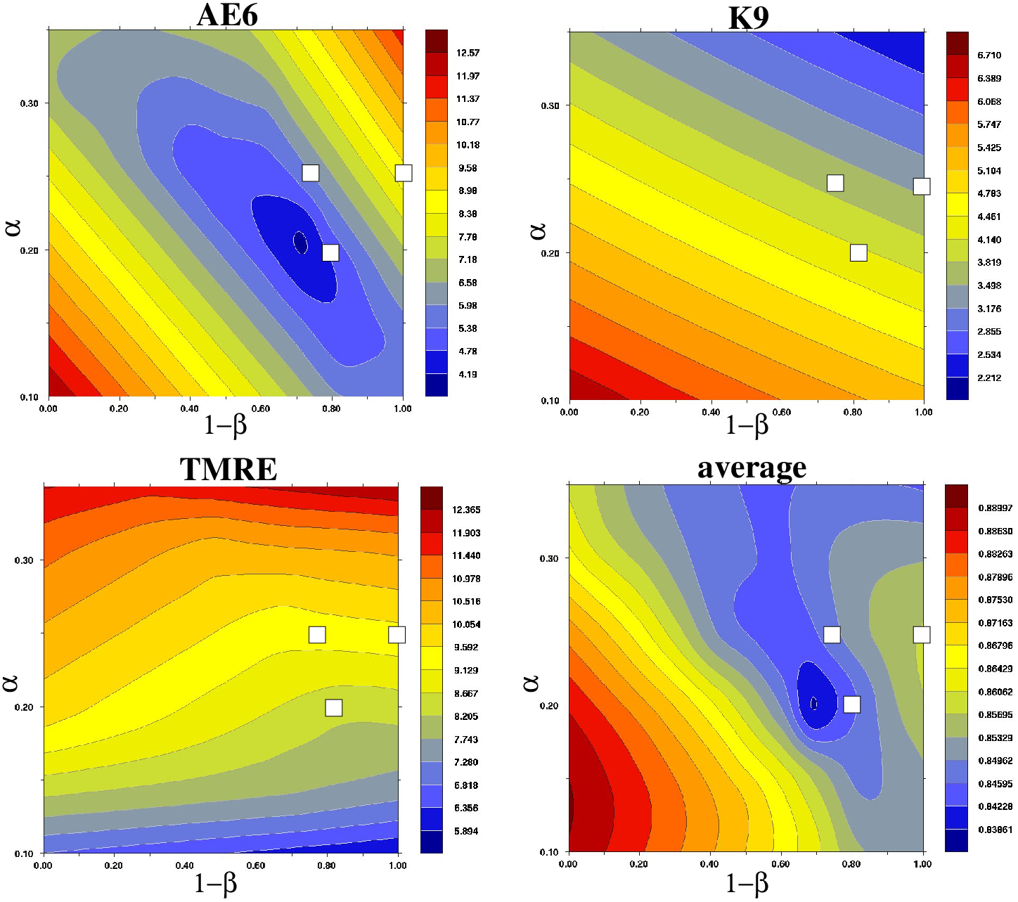
and we preform a scan of the values of the two parameters and to investigate the dependence of the results on the fraction of Hartree-Fock exchange and the correlation contribution. To this end we consider a minimal set of tests composed of the energy tests AE6 (atomization energies of small molecules), K9 (barrier heights and reaction energies of organic molecules), and TMRE (reaction energies of transition-metal complexes). These tests are in fact representative of the most important systems and properties as well as of the different trends observable in Table 2. To evaluate a global performance of the energy tests, which display rather different MAEs, we consider an average of the three tests after rescaling the result of each test as MAEMAE/(1+MAE). Note that the scaling has the two-fold purpose of making all the quantities comparable, so that a simple average is meaningful, and to enhance the differences between small values (which are the most interesting here).
The results of the scan for the energy tests are reported in Fig. 2. The plots show that indeed, as noticed when discussing Tab. 2, the different tests display different behaviors with respect to and . In particular, the barrier heights within the K9 test require a large fraction of Hartree-Fock exchange for an accurate description, while the opposite occurs in transition metals. On the other hand, atomization energies of organic molecules show an even more complex trend, requiring a delicate balance between exact exchange and correlation. Thus, overall the average performance has a complicated dependence on the two parameters. Nevertheless, it is possible to identify a clear minimum approximately corresponding to and , which is close to the definition of the functional with . Moreover, reasonably small average errors can be obtained for the family of parameters respecting the relation , which is close to the condition used in Eq. (6). Such a relation also shows that, as discussed in Section II.1, an accurate correlation functional to be used in hybrid functional should depend on the HF exchange contribution.

These results indicate the robustness of our construction based on the ansatz of Eq. (5) and the three imposed constraints. In particular, it is highlighted the importance of the satisfaction of the LDA linear response for the full XC functional, which is the constraint determining the condition in the functional of Eq. (6).
A somehow different situation is found concerning the geometry tests (MGHBL9 and MGNHBL11), which are reported in Fig. 3. In this case in fact a large and shallow minimum is observed for moderate values of the parameter and values ranging from 0.2 to 1. This indicates that reasonably small errors can be achieved by hybrid functionals including a sufficiently moderate fraction of Hartree-Fock exchange. In fact, for , the result of 4.4 mÅ is reasonably close to the global minimum of 3.7 mÅ.
Note also that the lines in both Figs. 2 and 3, which correspond to the hybrids which use the full PBEloc correlation, show a modest performance for all the tests. Such hybrids not only violates the LDA linear response, but also behave in the tail of the density as a pure exchange functional (because of the PBEloc construction). We recall that the correlation energy density plays an important role for asymptotic properties [109, 110]. Nevertheless, remarkably both Figs. 2 and 3 show that the best results are found for , which reveals an important significance of the PBEloc correlation as a tool for the construction of hybrid functionals. Thus, further development of semilocal correlation functionals more compatible with HF exchange, may further improve the quality of global hybrids.
IV.2 Semiempirical dispersion correction
| Functional | ||
|---|---|---|
| APBE | 1.242 | 0.930 |
| APBE0 | 1.259 | 0.921 |
| this work | 1.266 | 0.915 |
| this work | 1.258 | 0.923 |
| GGA | Hybrid | Hybrid | ||||
|---|---|---|---|---|---|---|
| Test | APBE-D3 | Eq. (6)-D3 | Eq. (10)-D3 | APBE0-D3 | Eq. (6)-D3 | Eq. (10)-D3 |
| hydrogen bonds (HB6) | 0.77 | 1.0 | 1.0 | 1.0 | 1.1 | 1.1 |
| dipole-dipole (DI6) | 0.91 | 0.73 | 0.73 | 0.69 | 0.69 | 0.69 |
| dihydrogen bonds (DHB23) | 1.3 | 1.2 | 1.2 | 1.0 | 1.1 | 1.1 |
| charge-transfer (CT7) | 2.9 | 1.8 | 1.8 | 1.5 | 1.6 | 1.6 |
| - stacking (pp5) | 0.2 | 0.18 | 0.18 | 0.20 | 0.21 | 0.21 |
| various non-covalent (S22) | 0.5 | 0.59 | 0.59 | 0.57 | 0.62 | 0.62 |
| isomerization (ISOL6) | 2.2 | 1.0 | 1.0 | 1.0 | 1.0 | 1.0 |
| small interfaces (SI12) | 4.5 | 5.8 | 5.7 | 7.6 | 6.6 | 6.5 |
To complete the construction of the hybrid functionals we considered to complement them with a semiempirical dispersion correction [111]. In fact, the dispersion interaction cannot be described neither by the Hartree-Fock exchange nor by any semilocal correlation. We implemented the dispersion correction through the DFT-D3 semiempirical model [111], fixing the two free parameters of the model by fitting to the MAE of the S22 test. The resulting parameters for different functionals are listed in Table 3. Note that because the S22 test only includes systems without any spin polarization the parameters of the D3 correction are the same for functionals defined by Eqs. (6) and (10).
The D3 dispersion correction is found to be well compatible with all the hybrid functionals, bringing a good improvement for dispersion dominated cases (i.e. S22 and pp5, where van der Waals interactions dominate or rather large systems are considered; see Tab. 4). Interestingly the semiempirical dispersion correction also reduces the MAE for ISOL6 and metal-organic interfaces (SI12). On the other hand, for the first four test in Tab. 4 where dispersion is not dominating, the D3 correction tends to slightly worsen the results for APBE and its hybrid variants. For all other tests (not reported Tab. 4) where dispersion does not play any relevant role, results are correctly left almost unchanged (data non reported).
V Conclusions
We have developed the global hybrids of the APBE exchange-correlation GGA functional [62]. The construction of these hybrids is based on the use of the PBEloc or zvPBEloc correlation functionals, to accompany the fraction of exact exchange, and on the recovery of the accurate LDA linear response. By a broad energetical and structural testing, including thermochemistry, organic geometry, atomization energies, reaction energies, and bond lengths of transition metal complexes, non-covalent interactions, isomerization, gold-molecules hybrid-interfaces, and dipole moments of organic molecules, we have shown that the best total performance is obtained by considering the hybrid using the zvPBEloc correlation (i.e Eq. (10)) and . We name this functional hAPBE. The hAPBE hybrid functional, shows an almost systematic improvement over the popular PBE0 and B3LYP hybrids, as well as over the recently proposed PBEmol0 functional. In fact, the hAPBE hybrid functional has a good accuracy for all the tests, showing a broad applicability, in contrast to the B3LYP functional which is modest for the transition metal complexes. Use of a semiempirical dispersion correction can bring further accuracy for problems where the dispersion interaction is especially relevant. Furthermore, the analysis of the hybrid parameters, summarized in Figs. 2 and 3, has shown that the LDA linear response is a powerful constraint, and that the PBEloc correlation plays a significant role in the functional performance. Thus the hAPBE functional can be regarded as an interesting tool for quantum chemistry applications. Whereas, the construction presented in this work, using a different correlation contribution to accompany the Hartree-Fock exchange and fulfilling the LDA linear response, appears to be an important strategy to develop more accurate hybrid functionals in the future.
In view of further improvements different semilocal correlation functionals with good compatibility with the Hartree-Fock exchange can be considered (e.g. GAPloc [68] or revTCA [6]). Alternatively, the replacement of GGAs with meta-GGAs can be considered in Eq. (4). We recall in fact that important recent work at the meta-GGA level has appeared. Hence, several accurate non-empirical (semi-empirical) functionals have been proposed, such as revTPSS [113], regTPSS [114], MGGA-MS [17], VT [115], and BLOC [66, 8, 10]. All of them represent good candidates for the construction of an accurate meta-GGA hybrid, using the method proposed in the present paper. In particular the BLOC functional uses a correlation term (TPSSloc [66]) which has been derived from the PBEloc GGA. Thus, this functional appears as the most natural choice for future studies.
VI Appendix
In this Appendix we analyze the coupling-constant-resolved XC potential energy formula in Eqs. (2) and (4) for atomic systems. As a reference we consider the coupling-constant-resolved XC potential energy of the interaction-strength interpolation (ISI) model (), a high-level method constructed from exact conditions [79].
The differences between the various approximate and the reference, as functions of , for several neutral atoms, are reported in 4. In addition we consider also the Ne8+ ion as an example for the high-density limit case. For all atoms we report also the exact behavior , where is the second-order Görling-Levy perturbation theory correlation (GL2) [80, 81], for small values of . Note that for Ne8+ this behavior becomes almost exact over the whole range of values.

The data in 4 show that the PBE0 ansatz is correct only at and in the close proximity of this point (by construction), whereas it shows a significant inaccuracy for larger values. The results are much improved for all atoms considered when the semilocal DFT approximation is changed from PBE to APBE (APBE0 curve). In this case in fact a closer behavior to the reference is obtained over the whole range of values. By construction, both and are exact at , while at , they recover the GGA behaviors, and [33]. As shown in Fig. 4, significantly improves over at , and consequently the APBE0 hybrid is more realistic.
Then we consider the ansatz introduced in Eq. (4). The curves labelled “” and “” in 4 clearly show that the correlation correction has a non negligible effect only for and that, for all system considered, a significant improvement is obtained for close to 1. In particular an almost vanishing error for is obtained for He and Ne.
References
- [1] Hohenberg, P.; Kohn, W. Phys. Rev. 1964, 136, B864-B871.
- [2] Kohn, W.; Sham, L. J. Phys. Rev. 1965, 140, A1133-A1138.
- [3] Perdew J. P.; Schmidt, K. AIP Conf. Proc. 2001, 577, 1-20.
- [4] Scuseria, G. E.; Staroverov, V. N. In Theory and Applications of Computational Chemistry: The First 40 Years (A Volume of Technical and Historical Perspectives); Dykstra, C. E.; Frenking, G.; Kim, K. S.; Scuseria, G. E., Eds.; Elsevier: Amsterdam, 2005; Chapter 24, pp 669-724.
- [5] Tognetti, V.; Cortona, P.; Adamo, C. J. Chem. Phys. 2008, 128, 034101.
- [6] Tognetti, V.; Cortona, P.; Adamo, C. Chem. Phys. Lett. 2008, 460, 536-539.
- [7] Bremond, E.; Pilard, D.; Ciofini, I.; Chermette, H.; Adamo, C.; Cortona, P. Theor. Chem. Acc. 2012, 131, 1184.
- [8] Constantin, L. A.; Fabiano, E.; Della Sala, F. J. Chem. Theory Comput. 2013, 9, 2256-2263.
- [9] Constantin, L. A.; Chiodo, L.; Fabiano, E.; Bodrenko, I.; Della Sala, F. Phys. Rev. B 2011, 84, 045126.
- [10] Constantin, L. A.; Fabiano, E.; Della Sala, F. Phys. Rev. B 2013, 88, 125112.
- [11] Armiento R.; Mattsson, A. E. Phys. Rev. B 2005, 72, 085108.
- [12] Mattsson, A. E.; Armiento, R. Phys. Rev. B 2009, 79, 155101.
- [13] Pittalis, S.; Räsänen, E.; Vilhena, J. G.; Marques, M. A. L. Phys. Rev. A 2009, 79, 012503.
- [14] del Campo, J. M.; Gázquez, J. L.; Trickey, S.; Vela, A. Chem. Phys. Lett. 2012, 543, 179-183.
- [15] Krieger, J. B.; Chen, J.; Kurth, S. In Density Functional Theory and its Applications to Materials; van Doren, V.; van Alsenoy, C. P. G., Eds.; Plenum Press: New York, 2000.
- [16] Zhao Y.; Truhlar, D. G. J. Chem. Phys. 2006, 125, 194101.
- [17] Sun, J.; Xiao, B.; Ruzsinszky, A. J. Chem. Phys. 2012, 137, 051101.
- [18] Chiodo, L.; Constantin, L. A.; Fabiano, E.; Della Sala, F. Phys. Rev. Lett. 2012, 108, 126402.
- [19] Tognetti, V.; Cortona, P.; Adamo, C. Theor. Chem. Account 2009, 122, 257.
- [20] Tognetti, V.; Adamo, C.; Cortona, P. Interdiscip. Sci. Comput. Life Sci. 2010, 2, 163-168.
- [21] Janesko, B. G.; Scuseria, G. E. J. Chem. Phys. 2008, 128, 244112.
- [22] Cohen, A. J.; Mori-Sánchez, P.; Yang, W. Chem. Rev. 2012, 112, 289-320.
- [23] Fabiano, E.; Constantin, L. A.; Della Sala, F. Int. J. Quantum Chem. 2013, 113, 673-682. Fabiano, E.; Constantin, L. A.; Della Sala, F. Int. J. Quantum Chem. 2013, 113, 1600.
- [24] Grabowski, I.; Teale, A. M.; Śmiga, S.; Bartlett, R. J. J. Chem. Phys. 2011, 135, 114111.
- [25] Grabowski, I.; Teale, A. M.; Fabiano, E.; Śmiga, S.; Buksztel, A.; Della Sala, F. Mol. Phys. 2014, 112, 700-710.
- [26] Becke, A. D. J. Chem. Phys. 1993, 98, 1372.
- [27] Becke, A. D. J. Chem. Phys. 1996, 104, 1040.
- [28] Savin, A. In Recent Developments and Applications of Modern Density Functional Theory, Seminario, J. M. Ed.; Elsevier: Amsterdam, 1996; pp. 327-357.
- [29] Iikura, H.; Tsuneda, T.; Yanai, T.; Hirao, K. J. Chem. Phys. 2001, 115, 3540.
- [30] Vydrov, O. A.; Scuseria, G. E. J. Chem. Phys. 2006, 125, 234109.
- [31] Zhao Y.; Truhlar, D. G. Theor. Chem. Acc. 2008, 120, 215-241.
- [32] Zhao, Y.; Schultz, N. E.; Truhlar, D. G. J. Chem. Phys. 2005, 123, 161103.
- [33] Perdew, J. P.; Ernzerhof, M.; Burke, K. J. Chem. Phys. 1996, 105, 9982.
- [34] Adamo, C.; Barone, V. J. Chem. Phys. 1999, 110, 6158.
- [35] Ernzerhof M.; Scuseria, G. E. J. Chem. Phys. 1999, 110, 5029.
- [36] Cortona, P. J. Chem. Phys. 2012, 136, 086101.
- [37] Guido, C. A.; Brémond, E.; Adamo, C.; Cortona, P. J. Chem. Phys. 2013, 138, 021104.
- [38] Hermet, J.; Cortona, P.; Adamo, C. Chem. Phys. Lett. 2012, 519-520, 145-149.
- [39] Haunschild, R.; Janesko, B. G.; Scuseria, G. E. J. Chem. Phys. 2009, 131, 154112.
- [40] Haunschild, R.; Perdew, J. P.; Scuseria, G. E. J. Chem. Phys. 2012, 137, 224104.
- [41] Arbuznikov, A. V.; Kaupp, M. Chem. Phys. Lett. 2007, 440, 160-168.
- [42] Arbuznikov, A. V.; Kaupp, M. J. Chem. Phys. 2012, 136, 014111.
- [43] Arbuznikov, A. V.; Kaupp, M. Int. J. Quantum Chem. 2011, 111, 2625-2638.
- [44] Haunschild, R.; Henderson, T. M.; Jiménez-Hoyos, C. A.; Scuseria, G. E. J. Chem. Phys. 2010, 133, 134116.
- [45] Haunschild R.; Scuseria, G. E. J. Chem. Phys. 2010, 132, 224106.
- [46] Perdew, J. P.; Staroverov, V. N.; Tao, J.; Scuseria, G. E. Phys. Rev. A 2008, 78, 052513.
- [47] Odashima, M. M.; Capelle, K. Phys. Rev. A 2009, 79, 062515.
- [48] Haunschild, R.; Odashima, M. M.; Scuseria, G. E.; Perdew, J. P.; Capelle, K. J. Chem. Phys. 2012, 136, 184102.
- [49] Huang, Y.-W.; Lee, S.-L. Chem. Phys. Lett. 2010, 492, 98-102.
- [50] Dickson, R. M.; Becke, A. D. J. Chem. Phys. 2005, 123, 111101.
- [51] Johnson, E. R.; Becke, A. D. J. Chem. Phys. 2005, 123, 024101.
- [52] Becke, A. D. J. Chem. Phys. 2005, 122, 064101.
- [53] Johnson, E. R.; Becke, A. D.; Sherrill, C. D.; DiLabio, G. A. J. Chem. Phys. 2009, 131, 034111.
- [54] Mori-Sánchez, P.; Cohen, A. J.; Yang W. J. Chem. Phys. 2006, 124, 091102.
- [55] Karton, A.; Tarnopolsky, A.; Lamere, J. F.; Schatz, G. C.; Martin, J. M. J. Phys. Chem. A 2008, 112, 12868-12886.
- [56] Schwabe, T.; Grimme, S. Phys. Chem. Chem. Phys. 2007, 9, 3397-3406.
- [57] Grimme S.; Neese, F. J. Chem. Phys. 2007, 127, 154116.
- [58] Becke, A. D. Phys. Rev. A 1998, 38, 3098.
- [59] Lee, C.; Yang, W.; Parr, R. G. Phys. Rev. B 1988, 37, 785.
- [60] Becke, A. D. J. Chem. Phys. 1993, 98, 5648.
- [61] Stephens, P. J.; Devlin, J. F.; Chabalowski, C. F.; Frisch, M. J. J. Phys. Chem. 1994, 98, 11623.
- [62] Constantin, L. A.; Fabiano, E.; Laricchia, S.; Della Sala, F. Phys. Rev. Lett. 2011, 106, 186406.
- [63] Fabiano, E.; Constantin, L. A.; Della Sala, F. J. Chem. Theory Comput. 2011, 7, 3548-3559.
- [64] Arbuznikov, A. V.; Kaupp, M. J. Chem. Phys. 2008, 128, 214107.
- [65] Sharkas, K.; Toulose, J.; Savin, A. J. Chem. Phys. 2011, 134, 064113.
- [66] Constantin, L. A.; Fabiano, E.; Della Sala, F. Phys. Rev. B 2012, 86, 035130.
- [67] Constantin, L. A.; Fabiano, E.; Della Sala, F. J. Chem. Phys. 2012 137, 194105.
- [68] Fabiano, E.; Trevisanutto, P. E.; Terentjevs, A.; Constantin, L. A. J. Chem. Theory Comput. 2014, 10, 2016-2026.
- [69] Moroni, S.; Ceperley, D. M.; Senatore, G. Phys. Rev. Lett. 1995, 75, 689.
- [70] Ortiz, G. Phys. Rev. B 1992, 45, 11328.
- [71] Perdew, J. P.; Burke, K.; Ernzerhof, M. Phys. Rev. Lett. 1996, 77, 3865.
- [72] Cancio, A. C.; Wagner, C. E.; Wood, S. A. Int. J. Quantum Chem. 2012, 112, 3796-3806.
- [73] del Campo, J. M.; Gázquez, J. L.; Trickey, S. B.; Vela, A. J. Chem. Phys. 2012, 136, 104108.
- [74] Elliott, P.; Burke, K. Can. J. Chem. 2009, 87, 1485-1491.
- [75] Lee, D.; Constantin, L. A.; Perdew, J. P.; Burke, K. J. Chem. Phys. 2009, 130, 034107.
- [76] Staroverov, V. E.; Scuseria, G. E.; Tao, J.; Perdew, J. P. J. Chem. Phys. 2003, 119, 12129.
- [77] Guido, C. A.; Cortona, P.; Mennucci, B.; Adamo, C. J. Chem. Theory Comput. 2013, 9, 3118-3126.
- [78] Guido, C. A.; Cortona, P.; Adamo, C. J. Chem. Phys. 2014, 140, 104101.
- [79] Seidl, M.; Perdew, J. P.; Kurth, S. Phys. Rev. Lett. 2000, 84, 5070.
- [80] Görling, A.; Levy, M. Phys Rev B 1993, 47, 13105.
- [81] Seidl, M.; Perdew, J. P.; Levy, M. Phys. Rev. A 1999, 59, 51.
- [82] Lynch, B. J.; Truhlar, D. G. J. Phys. Chem. A 2003, 107, 8996-8999.
- [83] Haunschild, R.; Klopper, W. Theor. Chem. Acc. 2012, 131, 1112.
- [84] Lynch, B. J.; Truhlar, D. G. J. Phys. Chem. A 2003, 107, 3898-3906.
- [85] Goerigk, L.; Grimme, S. J. Chem. Theory Comput. 2010, 6, 107-126.
- [86] Goerigk, L.; Grimme, S. Phys. Chem. Chem. Phys. 2011, 13, 6670-6688.
- [87] Parthiban, S.; Martin, J. M. L. J. Chem. Phys. 2001, 114, 6014.
- [88] Martin, J. M. L.; de Oliveira, G. J. Chem. Phys. 1999, 111, 1843.
- [89] Zhao, Y.; Truhlar, D. G. J. Phys. Chem. A 2006, 110, 10478-10486.
- [90] Curtiss, L. A.; Raghavachari, K.; Trucks, G. W.; Pople, J. A. J. Chem. Phys. 1991, 94, 7221.
- [91] Zhao, Y.; Lynch, B. J.; Truhlar, D. G. J. Phys. Chem. A 2004, 108, 2715-2719.
- [92] Zhao, Y.; González-García, N.; Truhlar, D. G. J. Phys. Chem. A 2005, 109, 2012-2018.
- [93] Zhao, Y.; Truhlar, D. G. J. Chem. Phys. 2006, 125, 194101.
- [94] Biczysko, M.; Panek, P.; Scalmani, G.; Bloino, J.; Barone, V. J. Chem. Theory Comput. 2010, 6, 2115-2125.
- [95] Furche, F.; Perdew, J. P. J. Chem. Phys. 2006, 124, 044103.
- [96] Constantin, L. A.; Fabiano, E.; Della Sala, F. Phys. Rev. B 2011, 84, 233103.
- [97] Fabiano, E.; Constantin, L. A.; Della Sala, F. J. Chem. Phys. 2011, 134, 194112.
- [98] Bühl, M.; Kabrede, H. J. Chem. Theory Comput. 2006, 2, 1282-1290.
- [99] Zhao, Y.; Truhlar, D. G. J. Chem. Theory Comput. 2005, 1, 415-432.
- [100] Fabiano, E.; Constantin, L. A.; Della Sala, F. J. Chem. Theory Comput. 2014, 10, 3151-3162.
- [101] Jurečka, P.; Sponer, J.; Cerny, J.; Hobza, P. Phys. Chem. Chem. Phys. 2006, 8, 1985-1993.
- [102] Marshall, M. S.; Burns, L. A.; Sherrill, C. D. J. Chem. Phys. 2011, 135, 194102.
- [103] Luo, S.; Zhao, Y.; Truhlar, D. G. Phys. Chem. Chem. Phys. 2011, 13, 13683-13689.
- [104] Peverati, R.; Truhlar, D. G. J. Chem. Theory Comput. 2012, 8, 2310-2319.
- [105] TURBOMOLE, V6.3; TURBOMOLE GmbH: Karlsruhe, Germany, 2011. Available from http://www.turbomole.com (accessed August 2014).
- [106] Weigend, F.; Furche, F.; Ahlrichs, R. J. Chem. Phys. 2003, 119, 12753.
- [107] Weigend, F.; Ahlrichs, R. Phys. Chem. Chem. Phys. 2005, 7, 3297-3305.
- [108] Paier, J.; Marsman, M.; Kresse, G. J. Chem. Phys. 2007, 127, 024103.
- [109] Constantin L. A.; Pitarke, J. M. Phys. Rev. B 2011, 83, 075116.
- [110] Horowitz, C. M.; Constantin, L. A.; Proetto, C. R.; Pitarke, J. M. Phys. Rev. B 2009, 80, 235101.
- [111] Grimme, S.; Antony, J.; Ehrlich, S.;. Krieg, H. J. Chem. Phys. 2010, 132, 154104.
- [112] Tao, J.; Perdew, J. P.; Staroverov, V. N.; Scuseria, G. E. Phys. Rev. Lett 2003, 91, 146401.
- [113] Perdew. J. P.; Ruzsinsky, A.; Csonka, G. I.; Constantin, L. A.; Sun, J. Phys. Rev. Lett. 2009, 103, 026403-026407; (E) Phys. Rev. Lett. 2011, 106, 179902.
- [114] Ruzsinszky, A.; Sun, J.; Xiao, B.; Csonka, G. I. J. Chem. Theory. Comput. 2012, 8, 2078-2087.
- [115] del Campo, J. M. ; Gázquez, J. L. ; Trickey, S. B. ; Vela, A. Chem. Phys. Lett. 2012, 543, 179.