Pre-inflationary primordial perturbations

Yong Cai^1, Note: caiyong13@mails.ucas.ac.cn Affiliation: ¹ School of Physics, University of Chinese Academy of Sciences, Beijing 100049, China Yu-Tong Wang¹ Note: wangyutong12@mails.ucas.ac.cn Affiliation: ¹ School of Physics, University of Chinese Academy of Sciences, Beijing 100049, China Yun-Song Piao^1,2 Note: yspiao@ucas.ac.cn Affiliation: ¹ School of Physics, University of Chinese Academy of Sciences, Beijing 100049, China Affiliation: ² State Key Laboratory of Theoretical Physics, Institute of Theoretical Physics,
Chinese Academy of Sciences, P.O. Box 2735, Beijing 100190, China

Abstract

The large-scale power deficit in the cosmic microwave background fluctuations might be relevant with the physics of pre-inflation, a bounce, or a superinflationary phase preceding slow-roll inflation, which can provide a singular-free realization of inflation. We investigate the primordial perturbations from such pre-inflationary evolutions, which generally may consist of multiple phases with different background dynamics, and give a universal formula for the power spectrum of primordial perturbations in terms of the recursive Bogoliubov coefficients. We also apply our formula to corresponding cases and show how the intensity of large-scale power suppression is affected by the pre-inflationary physics.

I Introduction

As the paradigm of the early universe, inflation has been generally regarded as a possible solution of the horizon, flatness, entropy, homogeneity, isotropy and primordial monopole problems[1],[2],[3],[4]. But maybe far more attractive is that inflation can generate the primordial perturbations, which have grown into all the structures observed in our universe today. The observations of cosmic microwave background (CMB) by Planck and WMAP has provided us with more and more information of the early universe, which shows that the single field slow-roll inflationary model is more likely to be the right one.

However, a large-scale (or low- $l$ ) power deficit in CMB TT-mode spectrum observed by WMAP [5] and recently confirmed by the Planck Collaboration[6][7] with higher precision is not concordant with the standard slow-roll inflation. It is hard to attribute this power deficit to the foreground as it has been observed by experiments with higher and higher statistical significance. Though the cosmic variance could be a source of this deficit, it is still very likely that the large-scale anomalies are induced by the physics preceding inflation, as the larger are the scales of the perturbations, the earlier are the times corresponding to their horizons exiting.

The slow-roll inflation might last for just the minimal number of $e$ -folds, i.e., just enough [8], and thus the power deficit on a large scale may be attributed to the pre-inflationary non-slow-roll evolution. In this case, the Planck best-fit single-field inflationary model only actually provides a fit for the intermediate and small angular scales. After the WMAP1 data were released, some studies have been done in Refs.[9],[10],[11],[12],[13],[14],[15] along this line, and also recently [16],[17],[18],[19],[20],[21],[22],[23]; see Ref.[24] for a review.

However, it might be more interesting that the large-scale anomalies could be relevant with the physics solving the initial singularity problem of inflation [11],[19]. In the bouncing model (see, e.g., [25],[26] for reviews), initially the universe is in a contracting phase, and then it bounces into an expanding phase, which results in a solution to the cosmological singularity problem. In Refs.[11],[14],[15],[16],[17],[21], it was noticed that if the universe is initially in a contracting phase and after the bounce it begins to inflate, the power spectrum of primordial perturbations will get a large-scale cutoff, which may naturally explain the power deficit of the CMB TT-mode spectrum at low- $l$ ; see, e.g., [16] for details. In addition, it was also observed in [27] that if the pre-inflationary bounce actually occurs, the BB-mode correlation at low- $l$ is also suppressed, while the TB- and EB-mode correlations on a corresponding scale may be enhanced.

The superinflationary phase before slow-roll inflation may also provide a singular-free realization of inflation, which in the meantime explains the anomalies of the CMB power spectrum [18],[28]; see also [29],[30] for an almost flat pre-inflationary universe.

In the above pre-inflationary scenarios, e.g., [11],[16],[18], initially the primordial perturbation is deep inside the horizon, which naturally set itself in Bunch-Davies(BD) vacuum. This implies that we can calculate a large-scale power spectrum without any assumption for the initial state of primordial perturbations. However, it is possible that the pre-inflationary era might consist of multiple phases with different background evolution, e.g., [24]. In a certain sense, the introduction of multiple pre-inflationary phases may better simulate the physics of the pre-inflationary era, since due to the complexity of pre-inflationary physics, sometimes a single phase can hardly reflect the drastic change of the background parameters, e.g., [20]. Therefore, it is interesting to have a quantitative estimate for the power spectra of primordial perturbations from an arbitrary pre-inflationary era, involving the multiple phases with different background dynamics.

This paper is organized as follows. In Sec.IIA, we introduce the evolution of the pre-inflationary background, which we will focus on, consisting of multiple phases. We require that the primordial perturbations can be produced in these phases. In Sec.IIB, we perform a model-independent calculation for the primordial perturbations and give a universal formula for the power spectra of primordial perturbations in terms of the recursive Bogoliubov coefficients. In Sec.III, we apply our formula to the bounce inflation and the superinflation preceding slow-roll inflation and show how the intensity of the large-scale power suppression of a primordial spectrum is affected by the pre-inflationary physics. We will see that a large-scale suppressed primordial spectrum may result in the power deficit at low- $l$ in the CMB TT-mode spectrum; however, the intensity of the power suppression is model-dependent. Sec.IV is the discussion.

In Appendix A, we will investigate the Wronskian constraint for primordial perturbations and argue that in a certain sense the scenario with pre-inflationary era is equivalent to the inflation scenario with the non-Bunch-Davis initial state. In Appendix B, we will approximately estimate the spectra index of primordial perturbations produced in each phase.

II Pre-inflationary primordial perturbations

II.1 The pre-inflationary background

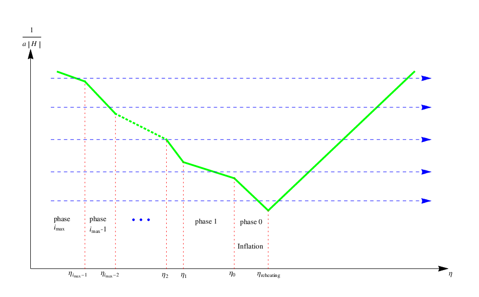
The pre-inflationary era may consist of multiple phases. We define the inflation as phase 0, the latest pre-inflationary phase as phase $1$ , and so on.

The cosmological evolution of phase $i$ is

a_{i}\sim\eta^{\frac{2}{1+3\omega_{i}}},\,\,\,{or}\,\,\,(-\eta)^{\frac{2}{1+3\omega_{i}}},

(1)

where $\omega_{i}=p_{i}/\rho_{i}$ is a constant, $\omega_{i}\neq-{1}/{3}$ , and $\eta=\int dt/a$ is the conformal time. The phase $i$ may be expanding or contracting.

However, noting the continuities of $a$ and $|H|$ , the evolutions of the inflation and phase $i$ can be rewritten as

a_{0}(\eta)=\frac{a_{0}(\eta_{0})}{1-{\cal H}_{inf}\cdot(\eta-\eta_{0})},

(2)

a_{i}(\eta)=a_{i}(\eta_{i-1})\left[1+\frac{1+3\omega_{i}}{2}{\cal H}_{i}(\eta_{i-1})\cdot(\eta-\eta_{i-1})\right]^{\frac{2}{1+3\omega_{i}}},

(3)

respectively, where $\eta_{0}$ is that at the onset of inflation, ${\cal H}_{inf}={\cal H}_{0}(\eta_{0})$ is the conformal Hubble parameter during slow-roll inflation, and $\eta_{i-1}$ is the matching time between phase $i$ and phase $i-1$ , which signals the onset of phase $i-1$ .

It seems that $\omega_{i}$ is arbitrary. However, if we require that initially all perturbation modes are in the BD state, which is right only if its wavelength $\lambda\ll{1/{\cal H}}$ , $\omega_{i}$ will be constrained. That the perturbation mode with $\lambda\sim 1/k$ extends outside the horizon in phase $i$ marks the primordial perturbation that is produced in this phase, which requires ${\cal H}_{i}(\eta_{i})<k<{\cal H}_{i}(\eta_{i-1})$ . Thus $|{\cal H}_{i}(\eta)|$ must increase with time, which implies

	$\displaystyle\omega_{i}$	$\displaystyle<$	$\displaystyle-1/3~\,\,\,\,for\,\,{{\rm the}}\,\,{{\rm expanding}}\,\,{{\rm phase}},$
	$\displaystyle or\,\,\,\omega_{i}$	$\displaystyle>$	$\displaystyle-1/3~\,\,\,\,for\,\,{{\rm the}}\,\,{{\rm contracting}}\,\,{{\rm phase}}.$		(4)

Or equally in other words, (4) must be satisfied to guarantee the primordial perturbations that can be produced during phase $i$ . The slow-roll inflation is the evolution with $\omega\simeq-1$ , which satisfies (4).

In general, there may be multiple pre-inflationary phases. Any one of them might be a contracting phase or an expanding phase. Therefore, there are two kinds of typical scenarios which have aroused lots of interests, i.e., the bouncing scenario and the superinflation scenario, which we will focus on in Secs. III.A and III.B.

In the bouncing scenario, a bounce happened near the end of the contracting phase then was followed by an expanding phase with $\omega<-1/3$ . The bounce may be implemented by applying a higher-order derivative field [31],[32],[33],[34], which is ghost-free, and also viscous fluid [35] and modified gravity [36],[37],[38],[39],[40].

The expansion with $\omega<-1$ is called superinflation, which is similar to the emergent scenario and describes a monotonically expanding universe with increasing energy density. The primordial perturbations generated during the superinflation have been studied earlier in Refs.[41],[42]. The case with $\omega\ll-1$ corresponds to the slow expansion scenario, which has been proposed in Ref.[44] (see also [45],[46] for the genesis scenario) and investigated in detail in Refs.[47],[48]. It is shown in Ref.[48] that there is no ghost instability during superinflation. Thus the pre-inflationary universe may also be superinflating. It is interesting to notice that both bounce and superinflation preceding slow-roll inflation may provide a singular-free realization of inflation.

However, if the pre-inflationary era is the expanding phase with $\omega=1$ characterized by fast-rolling dominance, e.g., [9],[49],[50],[51], except for the initial fast-roll inflation, e.g., [52], or the expanding phase with radiation dominance [10],[13], initially the perturbation mode should be outside the horizon, so it is not clear how to set its initial condition. It is possible that its initial value is set in a phase preceding fast-rolling dominance; however, this phase is still required to satisfy (4), e.g., a higher energy inflation preceding the fast-rolling phase [53]; see [24] for comments, and see also [23] for a domain wall or cosmic string phase. Here, we will not involve this issue and will assume that all pre-inflationary phases satisfy (4), which assures initially all perturbation modes are naturally set in BD vacuum and each phase may contribute to the production of primordial perturbations with the certain range of wave numbers.

We qualitatively plot the evolutions of background and perturbation modes, which we will focus on, in Fig.1.

Refer to caption — Figure 1: The green line denotes the evolution of the comoving Hubble radius $\frac{1}{a|H|}$ , and $\eta_{i}$ signals the onset of phase $i$ . The blue dashed lines denote the evolutions of the primordial perturbations.

II.2 The power spectrum of pre-inflationary perturbations

The equation of the primordial perturbation $\cal R$ is [54],[55]

u^{\prime\prime}+\left(c_{s}^{2}k^{2}-\frac{z^{\prime\prime}}{z}\right)u=0,

(5)

where $u\equiv z{\cal R}$ , the prime is the derivative with respect to conformal time, $z\equiv a\sqrt{2M_{p}^{2}\epsilon}/c_{s}$ [56], and $z\simeq a\sqrt{2M_{p}^{2}|\epsilon|}/c_{s}$ [48] for the superinflationary phase, and the definition of $\epsilon$ is $\epsilon\equiv-{\dot{H}}/{H^{2}}={3(1+\omega)\over 2}$ . We assume $c_{s}^{2}=1$ for simplicity.

In the slow-roll inflationary phase, we have

\frac{z^{\prime\prime}_{0}}{z_{0}}\simeq\frac{2{\cal H}_{inf}^{2}}{\left[1-{\cal H}_{inf}(\eta-\eta_{0})\right]^{2}},

(6)

the solution of Eq.(5) is

\displaystyle u_{0}

\displaystyle=

\displaystyle\sqrt{-k{\eta}_{eff_{0}}}\left[C_{0,1}H^{(1)}_{3/2}\left(-k{\eta}_{eff_{0}}\right)+C_{0,2}H^{(2)}_{3/2}\left(-k{\eta}_{eff_{0}}\right)\right],

(7)

where $H^{(1)}_{3/2}$ and $H^{(2)}_{3/2}$ are the $(3/2)$ th order Hankel functions of the first and second kinds, respectively, and ${\eta}_{eff_{0}}=\eta-\eta_{0}-\frac{1}{{\cal H}_{inf}}$ .

In pre-inflationary phase $i$ , we have

\frac{z_{i}^{\prime\prime}}{z_{i}}\simeq\frac{(1-3\omega_{i}){\cal H}_{i}^{2}(\eta_{i-1})}{2\left[1+\frac{1+3\omega_{i}}{2}{\cal H}_{i}(\eta_{i-1})\cdot(\eta-\eta_{i-1})\right]^{2}},

(8)

the solution of Eq.(5) is

\displaystyle u_{i}=\sqrt{-k{\eta}_{eff_{i}}}\left[C_{i,1}H^{(1)}_{v_{i}}\left(-k{\eta}_{eff_{i}}\right)+C_{i,2}H^{(2)}_{v_{i}}\left(-k{\eta}_{eff_{i}}\right)\right],

(9)

where $v_{i}=\frac{3}{2}\left|\frac{1-\omega_{i}}{1+3\omega_{i}}\right|$ . $H^{(1)}_{v_{i}}$ and $H^{(2)}_{v_{i}}$ are the $v_{i}$ th order Hankel functions of the first and second kinds, respectively, and ${\eta}_{eff_{i}}=\eta-\eta_{i-1}+\frac{2}{(1+3\omega_{i}){\cal H}_{i}(\eta_{i-1})}$ . In fact, Eq.(7) can be obtained from Eq.(9) while $i=0$ , but $\eta_{i-1}$ should be replaced by $\eta_{0}$ .

Here, we require that around and at the matching surface besides there is not the ghost instability; there is also not gradient instability, i.e., $c_{s}^{2}>0$ . In this case, the perturbation can continuously pass through the matching surface between two adjacent phases, and its spectrum is insensitive to the physical details around the matching surface; see e.g., [57] for the bounce. The coefficients $C_{i}$ in Eqs.(7) and (9) are determined by requiring the continuity of $u$ and $u^{\prime}$ at the matching surface. We can write the coefficients $C_{i,1}$ and $C_{i,2}$ of phase $i$ recursively as

	$\displaystyle\left(\begin{array}[]{ccc}C_{i,1}\\ C_{i,2}\end{array}\right)$	$\displaystyle=$	$\displaystyle{\cal M}^{(i,i+1)}\times\left(\begin{array}[]{ccc}C_{i+1,1}\\ C_{i+1,2}\end{array}\right)$
		$\displaystyle=$	$\displaystyle{\cal M}^{(i,i+1)}\times{\cal M}^{(i+1,i+2)}\times\cdots\times{\cal M}^{(i_{max}-1,i_{max})}\times\left(\begin{array}[]{ccc}C_{i_{max},1}\\ C_{i_{max},2}\end{array}\right),$

where the earliest phase is defined as the phase $i_{max}$ , and ${\cal M}^{(i,i+1)}=\left(\begin{array}[]{ccc}{\cal M}_{11}&{\cal M}_{12}\\ {\cal M}_{21}&{\cal M}_{22}\end{array}\right)$ is the recursive matrix, which is given by

$\displaystyle{\cal M}_{11}$	$\displaystyle=$	$\displaystyle\frac{i\pi\sqrt{xy}}{8}\bigg\{\left[-H^{(1)}_{-1+v_{i+1}}(y)+H^{(1)}_{1+v_{i+1}}(y)\right]H^{(2)}_{v_{i}}(x)+\left[H^{(2)}_{-1+v_{i}}(x)-H^{(2)}_{1+v_{i}}(x)\right]H^{(1)}_{v_{i+1}}(y)$
	$\displaystyle+$	$\displaystyle(x^{-1}-y^{-1})H^{(2)}_{v_{i}}(x)H^{(1)}_{v_{i+1}}(y)\bigg\},$
$\displaystyle{\cal M}_{12}$	$\displaystyle=$	$\displaystyle\frac{i\pi\sqrt{xy}}{8}\bigg\{\left[-H^{(2)}_{-1+v_{i+1}}(y)+H^{(2)}_{1+v_{i+1}}(y)\right]H^{(2)}_{v_{i}}(x)+\left[H^{(2)}_{-1+v_{i}}(x)-H^{(2)}_{1+v_{i}}(x)\right]H^{(2)}_{v_{i+1}}(y)$
	$\displaystyle+$	$\displaystyle(x^{-1}-y^{-1})H^{(2)}_{v_{i}}(x)H^{(2)}_{v_{i+1}}(y)\bigg\},$
$\displaystyle{\cal M}_{21}$	$\displaystyle=$	$\displaystyle\frac{i\pi\sqrt{xy}}{8}\bigg\{\left[H^{(1)}_{-1+v_{i+1}}(y)-H^{(1)}_{1+v_{i+1}}(y)\right]H^{(1)}_{v_{i}}(x)-\left[H^{(1)}_{-1+v_{i}}(x)-H^{(1)}_{1+v_{i}}(x)\right]H^{(1)}_{v_{i+1}}(y)$
	$\displaystyle-$	$\displaystyle(x^{-1}-y^{-1})H^{(1)}_{v_{i}}(x)H^{(1)}_{v_{i+1}}(y)\bigg\},$
$\displaystyle{\cal M}_{22}$	$\displaystyle=$	$\displaystyle\frac{i\pi\sqrt{xy}}{8}\bigg\{\left[H^{(2)}_{-1+v_{i+1}}(y)-H^{(2)}_{1+v_{i+1}}(y)\right]H^{(1)}_{v_{i}}(x)-\left[H^{(1)}_{-1+v_{i}}(x)-H^{(1)}_{1+v_{i}}(x)\right]H^{(2)}_{v_{i+1}}(y)$	(18)
	$\displaystyle-$	$\displaystyle(x^{-1}-y^{-1})H^{(1)}_{v_{i}}(x)H^{(2)}_{v_{i+1}}(y)\bigg\},$	(18)

where $x=-\frac{2k}{(1+3\omega_{i}){\cal H}_{i}(\eta_{i})}$ and $y=-\frac{2k}{(1+3\omega_{i+1}){\cal H}_{i+1}(\eta_{i})}$ . When $i=0$ , $\eta_{i-1}$ should be replaced with $\eta_{0}$ . A result similar to (18) was obtained in [24].

In the earliest phase, the coefficients $C_{i_{max},1}$ and $C_{i_{max},2}$ are determined by the initial condition. When $k^{2}\gg\frac{z_{i_{max}}^{\prime\prime}}{z_{i_{max}}}$ , the perturbation mode is deep inside the horizon, which is set in BD vacuum,

u\sim\frac{1}{\sqrt{2k}}e^{-ik\eta}.

(19)

When $k^{2}\gg\frac{z_{i_{max}}^{\prime\prime}}{z_{i_{max}}}$ , $u_{i_{max}}$ given in Eq.(9) should approximate to the form in Eq.(19). Thus, we get

C_{i_{max},1}=\frac{\sqrt{\pi}}{2\sqrt{k}},\,\,\,C_{i_{max},2}=0.

(20)

Obviously, $C_{i_{max},1}$ and $C_{i_{max},2}$ satisfy the so-called Wronskian (or canonical normalization) constraint (see e.g. [58], [59])

\frac{4k}{\pi}\left(|C_{i_{max},1}|^{2}-|C_{i_{max},2}|^{2}\right)=1.

(21)

And actually, for the following phase $i$ , $C_{i,1}$ and $C_{i,2}$ will always satisfy the Wronskian constraint, which will be proved in Appendix A. $C_{i,1}$ and $C_{i,2}$ are related to the so-called Bogoliubov coefficients by Eq.(36).

The power spectrum of $\cal R$ is

{\cal P}_{\cal R}=\frac{k^{3}}{2\pi^{2}}\left|\frac{u_{0}}{z_{0}}\right|^{2}.

(22)

After substituting Eq.(7) into Eq.(22) and requiring $\left|k(\eta-\eta_{0})-\frac{k}{{\cal H}_{inf}}\right|\ll 1$ , we get a universal formula

{\cal P}_{\cal R}={\cal P}^{inf}_{\cal R}\frac{4}{\pi}k\left|C_{0,1}-C_{0,2}\right|^{2},

(23)

where ${\cal P}^{inf}_{\cal R}=\frac{1}{2M_{p}^{2}\epsilon_{inf}}\left(\frac{H_{inf}}{2\pi}\right)^{2}$ is the spectrum of the standard slow-roll inflation, $H_{inf}={{\cal H}_{0}(\eta_{0})}/{a_{0}(\eta_{0})}$ is the Hubble parameter during inflation, and in this sense actually ${\cal H}_{0}(\eta_{0})={\cal H}_{inf}$ . The spectral index of $\cal R$ is

n_{\cal R}=n_{inf}+\frac{d\ln(k\left|C_{0,1}-C_{0,2}\right|^{2})}{d\ln k},

(24)

where $n_{inf}={d\ln{\cal P}^{inf}_{\cal R}\over d\ln{k}}+1$ is the spectral index of slow-roll inflation, which is nearly unity.

The coefficients $C_{0,1}$ and $C_{0,2}$ are determined by the recursive Eq.(II.2), and thus the effects of all pre-inflationary phases are encoded in $C_{0,1}$ and $C_{0,2}$ , which are nontrivial. By calculating Eq.(23), it can be found that the perturbations produced in phase $i$ roughly have a power spectrum

{\cal P}_{\cal R}\sim k^{3-2v_{i}}.

(25)

We give a proof for this result in Appendix B. It is observed in Appendix B that the power spectrum of perturbations is Eq.(25) but modulated with a small oscillation, which is induced by the evolution of perturbation through the matching surface between adjacent phases.

III The large-scale power suppression

In this section, we will apply our universal formula (23) to the bounce inflation and the superinflation preceding slow-roll inflation, and show how the intensity of the large-scale power suppression in the CMB fluctuations is affected by the pre-inflationary evolution.

The large-scale power suppression requires that the $e$ -folding number of slow-roll inflation is just enough or less, and in the meantime the pre-inflationary era can contribute a strong blue-tilt spectrum. The spectral index of pre-inflationary perturbations is approximately

n_{\cal R}-1\simeq\frac{d\ln(k\left|C_{0,1}-C_{0,2}\right|^{2})}{d\ln k}.

(26)

Thus the intensity of suppression can be model dependent, since $|C_{0,1}-C_{0,2}|^{2}$ is different for different parameters $\omega_{i}$ and $\eta_{i}$ .

Here, we will focus on the cases that the pre-inflationary era consists of two phases, i.e., $i_{max}=2$ , and set ${\cal H}_{0}(\eta_{0})={\cal H}_{inf}$ and $\eta_{0}=0$ is the time at the onset of inflation; thus, we have $\eta<0$ in the pre-inflationary phases and $\eta>0$ in the inflationary phase. According to Sec.IIB, for $i_{max}=2$ , the solutions of Eq.(5) are

$\displaystyle u_{0}$	$\displaystyle=$	$\displaystyle\sqrt{-k\eta+\frac{k}{{\cal H}_{inf}}}\left[C_{0,1}H^{(1)}_{3/2}(-k\eta+\frac{k}{{\cal H}_{inf}})+C_{0,2}H^{(2)}_{3/2}(-k\eta+\frac{k}{{\cal H}_{inf}})\right],$
$\displaystyle u_{1}$	$\displaystyle=$	$\displaystyle\sqrt{-k\eta-\frac{2k}{(1+3\omega_{1}){\cal H}_{1}(0)}}\Big[C_{1,1}H^{(1)}_{v_{1}}(-k\eta-\frac{2k}{(1+3\omega_{1}){\cal H}_{1}(0)})$
		$\displaystyle\qquad\qquad\qquad\qquad\qquad\quad\,\,+C_{1,2}H^{(2)}_{v_{1}}(-k\eta-\frac{2k}{(1+3\omega_{1}){\cal H}_{1}(0)})\Big],$
$\displaystyle u_{2}$	$\displaystyle=$	$\displaystyle\frac{\sqrt{\pi}}{2}\sqrt{-\eta+\eta_{1}-\frac{2}{(1+3\omega_{2}){\cal H}_{2}(\eta_{1})}}H^{(1)}_{v_{2}}(-k\eta+k\eta_{1}-\frac{2k}{(1+3\omega_{2}){\cal H}_{2}(\eta_{1})}),$	(27)

respectively, where $\eta_{1}<0$ is the conformal time at the matching surface between phase $1$ and phase $2$ .

We define

P(\eta_{1},\omega_{1},\omega_{2})=\frac{{\cal P}_{\cal R}}{{\cal P}_{\cal R}^{inf}}=\frac{4}{\pi}k|C_{0,1}-C_{0,2}|^{2},

(28)

where according to Eq.(II.2), we have

\displaystyle\left(\begin{array}[]{ccc}C_{0,1}\\ C_{0,2}\end{array}\right)={\cal M}^{(0,1)}\times{\cal M}^{(1,2)}\times\left(\begin{array}[]{ccc}\frac{\sqrt{\pi}}{2\sqrt{k}}\\ 0\end{array}\right),

and the components of ${\cal M}^{(0,1)}$ , ${\cal M}^{(1,2)}$ can be obtained from Eq.(18). $P(\eta_{1},\omega_{1},\omega_{2})$ reflects the shape of the spectrum. We will check how the shape of the spectrum, as well as the intensity of suppression on a large scale, changes with the parameters $\eta_{1}$ , $\omega_{1}$ , and $\omega_{2}$ in the bounce inflation and the superinflation preceding slow-roll inflation.

III.1 The superinflationary phase before inflation

The superinflation is defined as the evolution with $\epsilon\equiv-{\dot{H}}/H^{2}<0$ or $\omega<-1$ , e.g., [41],[42],[43],[44]. The model with one single superinflationary phase $\omega=-{5}/{3}$ preceding slow-roll inflation has been built in string theory in Ref.[18]. In Refs.[29],[30], the pre-inflationary universe is in a slowly expanding genesis phase with $\epsilon\ll-1$ , which is almost Minkowski space. This genesis phase actually also belongs to the superinflation, but since $\epsilon\ll-1$ , the expansion is actually slow; see also [28] for the emergent universe.

We will fix phase 2 with $\omega_{2}=-{5}/{3}$ . Thus in a certain sense phase 1 actually corresponds to an intermediate phase, which obviously must also be expanding. The duration that this intermediate phase lasts is $\Delta\eta=|\eta_{1}|$ . Here, the parameter $\omega_{1}$ in phase 1 is model-dependent but should satisfy $\omega_{1}<-{1}/{3}$ . By requiring the continuity of $|{\cal H}|$ , we get

{\cal H}_{1}(0)={\cal H}_{inf}\,,\qquad{\cal H}_{2}(\eta_{1})=\frac{2{\cal H}_{inf}}{2+(1+3\omega_{1})\eta_{1}{\cal H}_{inf}},

(34)

where ${\cal H}_{inf}$ is determined by the amplitude of CMB fluctuations. Thus in equation set (27) only parameters $\eta_{1}$ and $\omega_{1}$ are left to be free.

We plot $P(\eta_{1},\omega_{1},-{5}/{3})$ in Fig.2 with different $\eta_{1}$ and $\omega_{1}$ . The black solid curve, i.e., $P(0,-1,-{5}/{3})$ , is the case with only one single superinflationary phase before slow-roll inflation, which has been studied in Ref.[18]. The perturbation mode with wavelength $1/k=1/{\cal H}_{inf}$ is that exiting the horizon at conformal time $\eta=0$ , i.e., the onset of inflation. In Fig.3, we plot $\bar{P}(\eta_{1},\omega_{1},-{5}/{3})$ by replacing $k$ with ${k}/{|\eta_{1}|}$ , which corresponds to move the suppression of the spectrum to a smaller scale.

In Fig.2, the effects of an intermediate phase between superinflation and slow-roll inflation is obvious, compared with the case without the intermediate phase. The first peaks in the dashed curves will left shift with the increase of the duration $|\eta_{1}|$ that the intermediate phase lasts. The height of the first peak will lower with the decrease of $\omega_{1}$ , since the first peak corresponds to $\frac{k}{{\cal H}_{inf}}<1$ while the spectrum is blue tilted. The power spectrum of perturbation from the intermediate phase , i.e. phase $1$ , is roughly ${\cal P}_{{\cal R}}\sim(\frac{k}{{\cal H}_{inf}})^{3-2v_{1}}$ , which will be proved in Appendix B.

III.2 The bounce inflation

The pre-inflationary universe may be contracting. After the bounce, the slow-roll inflation begins, which is the so-called bounce inflation scenario [11],[14],[15],[16],[17], [21] with $G$ -bounce, and [22] with the quintom. It has been found that in this scenario the power spectrum of primordial perturbations will get a large-scale cutoff, which may lead to the power deficit of CMB TT-mode on a large angular scale.

However, around the bounce the evolution of the universe is complicated. It might be possible that after the bounce the universe enters into an intermediate phase prior to the slow-roll inflation. We will check how the shape of the spectrum changes with this intermediate phase. We fixed $\omega_{2}=1$ and assume that the intermediate phase is characterized by the constant state parameter $\omega_{1}$ , which is model dependent but satisfies $\omega_{1}<-{1}/{3}$ . By requiring the continuity of $|{\cal H}|$ , we get

{\cal H}_{1}(0)={\cal H}_{inf}\,,\qquad{\cal H}_{2}(\eta_{1})=-\frac{2{\cal H}_{inf}}{2+(1+3\omega_{1})\eta_{1}{\cal H}_{inf}},

(35)

where ${\cal H}_{inf}$ is determined by the amplitude of CMB fluctuations. Thus in equation set (27) only parameters $\eta_{1}$ and $\omega_{1}$ are left to be free.

We plot $P(\eta_{1},\omega_{1},1)$ with different $\eta_{1}$ and $\omega_{1}$ in Fig.4, in which the black solid curves, i.e. $P(0,-1,1)$ , correspond to the bounce inflation studied explicitly in [11] [16]. In Fig.4, the effects of an intermediate phase between contraction and slow-roll inflation is obvious. The case is similar to III.1. In Fig.5, we plot $\bar{P}(\eta_{1},\omega_{1},1)$ by replacing $k$ with ${k}/{|\eta_{1}|}$ , which corresponds to move the suppression of the spectrum to a smaller scale. Actually, similar shapes of the power spectrum have also been obtained in Ref.[20].

IV Discussion

The large-scale power deficit in the CMB TT-mode spectrum may imply certain pre-inflationary physics, e.g., a contracting phase followed by the bounce or a superinflationary phase before slow-roll inflation, which can provide a singular-free realization of inflation. However, the physics of the pre-inflationary era might be complex; sometimes a single phase can hardly reflect the drastic change of the background dynamics. Thus it is interesting to have a quantitative estimate for the power spectrum of primordial perturbations from an arbitrary pre-inflationary era, involving multiple phases with different background dynamics.

We perform a model-independent calculation for the power spectrum of primordial perturbations produced during the pre-inflation with different background evolutions. We require the relevant physical quantities to continuously pass through the matching surface between adjacent phases, and we obtain a universal formula (23) for the primordial spectrum in terms of the recursive Bogoliubov coefficients.

We apply our formula to the bounce inflation and the superinflation preceding slow-roll inflation and show how the intensity of the CMB power suppression on the large scale is affected by the pre-inflationary physics. It is found that due to the existence of the intermediate phase, the intensity of the power suppression becomes model dependent.

We, with the power spectrum in Fig.4, plot the CMB TT-mode spectrum in Fig.6, in which Planck 2013 data are used and the model with an intermediate phase is called the extended bounce inflation. It has been found in Ref.[16] that the bounce inflation model can improve the fit to the data with $\Delta\chi_{\rm eff}^{2}\approx-4.6$ with respect to the standard inflation model with the power-law spectrum. Thus, it is interesting to have a global fitting analysis with the Planck new data, which is left in the upcoming work.

In addition, both the bounce inflation and the superinflation preceding slow-roll inflation may also explain a large dipole power asymmetry at low- $l$ in CMB TT-mode spectrum [16],[18]; see also other attempts [60],[61],[62],[63],[64],[65], as well as [66],[67]. Actually, there may also be dipole power asymmetry in CMB polarization [68],[69], which might be larger than those in the TT-mode power spectrum. Thus it is interesting to have an estimate for the dipole power asymmetry of CMB polarization in the scenarios discussed here.

For the sake of simplifying the analysis and algorithm, we have made several assumptions. We have divided the pre-inflationary evolution into multiple phases and assumed that each phase possesses a constant equation of state parameter, and the transitions from one phase to the next are instantaneous. But in reality, the equation of state parameter may be nonconstant, the transitions should be smooth, and the equation of state parameter should change smoothly. However, as long as there are long phases with approximately constant equation of state parameters and relatively quick transitions between the different phases, the approximation we adopted to simplify our analysis and algorithm is reasonable. Of course, the influence on the perturbations induced by a nonconstant equation of state parameter is interesting, and the effects of the modes that exit the Hubble radius near the transition from one phase to another are even more intriguing, which have been studied in [70],[71].

Throughout, we have used perturbation and background equations that are valid for general relativity (GR), since we lack the knowledge of the new physics that is needed for the pre-inflationary evolution. To implement bounce and superinflation evolutions in GR, we must violate the null energy condition(NEC) or require a closed universe. Otherwise, one must go beyond GR.

The violation of NEC in GR usually leads to ghosts, which indicate dangerous instability. One of the several ways to avoid ghosts is by introducing the higher-order derivative scalar field. In some ghost-free Galileon bounce or superinflation models, by delicately designing the Lagrangian, one can get the perturbation equation similar to ours in the form (see, e.g., [31],[48],[72]), in which the sound speed is constant, which is set as 1 here. In that case, our analysis is still able to approximately capture the bounce or superinflation dynamics. Additionally, in singular bounce models, e.g., the original ekpyrotic model, the background is GR and the perturbation equation does not need to be modified, until the scale factor $a(t)$ is so small that quantum gravity effects become important. Then, if the bounce period is short so that the link between the contracting phase and the expanding phase is approximately instantaneous just as we have assumed, our analysis is also approximately valid. However, in some kinds of modified gravity theories, in which the perturbation equations are modified, especially when higher-order terms of gravity appear in the perturbation equations, e.g., [73], our analysis will no longer be robust and will need to be revisited.

It is significant that recently in [74], some general results for the evolutions of perturbation modes during bounce have become available, which might be used to track the perturbations during the bounce. And obtaining the recursive matrix for some specific bouncing model to better understand how the modes evolve during this period is an interesting issue, which we will back to in the future.

We have assumed $c_{s}^{2}=1$ after Eq.(5), which is suitable for the cosmology driven by the scalar field. However, for an ideal fluid, $c_{s}^{2}=\omega$ , and for $\omega<0$ , it is negative which indicates an instability in the system. It is well known in thermal physics that a negative heat capacity typically implies that one is looking at thermal fluctuations around an incorrect (possibly tachyonic) vacuum. For $\omega<0$ , essentially the short wavelength fluctuations grow exponentially rather than oscillate. Actually, for scalar fields, $c_{s}^{2}$ may also be different from $1$ . The effects of varying sound speed on primordial perturbations has been studied; see, e.g., [75],[76]. But as long as $c_{s}^{2}$ is a positive constant during each phase, our result is not qualitatively altered.

When deriving (23), we assume that around and at matching surfaces the perturbation mode has no ghost and gradient instabilities. How to implement such a requirement is an interesting issue, e.g., [30],[57]. However, if this requirement is not satisfied, which actually is not allowed physically, the result of the perturbation spectrum will be strongly affected by the physical details around the matching surface.

Acknowledgments

We thank Zhi-Guo Liu for helpful discussions. This work is supported by NSFC, No.11222546, and National Basic Research Program of China, No.2010CB832804. We acknowledge the use of CAMB.

Appendix A: The Wronskian constraint for $C_{i,1}$ and $C_{i,2}$

Initially $k\ll{\cal H}$ , and the perturbation should be in its minimal energy state, i.e., BD vacuum. Thus, the BD vacuum is usually regarded as the initial state of the primordial perturbations. The effects of non-BD initial states on the primordial perturbation has been discussed in, e.g., Refs., [77],[78],[79],[80],[81],[82],[83],[84]. Here, the Bogoliubov coefficients are

	$\displaystyle\alpha_{i}=2\sqrt{\frac{k}{\pi}}C_{i,1},$
	$\displaystyle\beta_{i}=2\sqrt{\frac{k}{\pi}}C_{i,2}.$		(36)

The Wronskian (or canonical normalization) constraint requires $|\alpha_{i}|^{2}-|\beta_{i}|^{2}=1$ . The initial state, i.e., BD vacuum, corresponds to $\alpha_{i_{max}}=1$ and $\beta_{i_{max}}=0$ , i.e.,

C_{i_{max},1}=\frac{\sqrt{\pi}}{2\sqrt{k}},\qquad C_{i_{max},2}=0.

(37)

We will prove that if $C_{i_{max},1}$ and $C_{i_{max},2}$ satisfy the Wronskian constraint, for any phase $i$ , $C_{i,1}$ and $C_{i,2}$ also satisfy this constraint. This is equivalent to the statement that for any phase $i$ , if

\frac{4k}{\pi}\left(|C_{i+1,1}|^{2}-|C_{i+1,2}|^{2}\right)=1

(38)

is satisfied, we always have

\frac{4k}{\pi}\left(|C_{i,1}|^{2}-|C_{i,2}|^{2}\right)=1.

(39)

It equals the proof that

\displaystyle\left(\begin{array}[]{ccc}\overline{C}_{i,1}&\overline{C}_{i,2}\end{array}\right)\times\left(\begin{array}[]{ccc}1&0\\ 0&-1\end{array}\right)\times\left(\begin{array}[]{ccc}C_{i,1}\\ C_{i,2}\end{array}\right)=\left(\begin{array}[]{ccc}\overline{C}_{i+1,1}&\overline{C}_{i+1,2}\end{array}\right)\times\left(\begin{array}[]{ccc}1&0\\ 0&-1\end{array}\right)\times\left(\begin{array}[]{ccc}C_{i+1,1}\\ C_{i+1,2}\end{array}\right),

where $\overline{C}$ is the complex conjugation of $C$ . Because of

\displaystyle\left(\begin{array}[]{ccc}C_{i,1}\\ C_{i,2}\end{array}\right)={\cal M}^{(i,i+1)}\times\left(\begin{array}[]{ccc}C_{i+1,1}\\ C_{i+1,2}\end{array}\right),

we have

	$\displaystyle\left(\begin{array}[]{ccc}\overline{C}_{i,1}&\overline{C}_{i,2}\end{array}\right)$	$\displaystyle=$	$\displaystyle\left(\begin{array}[]{ccc}C_{i,1}\\ C_{i,2}\end{array}\right)^{{\dagger}}=\left(\begin{array}[]{ccc}C_{i+1,1}\\ C_{i+1,2}\end{array}\right)^{{\dagger}}\times\left({\cal M}^{(i,i+1)}\right)^{{\dagger}}$
		$\displaystyle=$	$\displaystyle\left(\begin{array}[]{ccc}\overline{C}_{i+1,1}&\overline{C}_{i+1,2}\end{array}\right)\times\left({\cal M}^{(i,i+1)}\right)^{{\dagger}}.$

Thus after substituting Eqs.(Appendix A: The Wronskian constraint for $C_{i,1}$ and $C_{i,2}$ ) and (Appendix A: The Wronskian constraint for $C_{i,1}$ and $C_{i,2}$ ) into Eq.(Appendix A: The Wronskian constraint for $C_{i,1}$ and $C_{i,2}$ ), we have

\displaystyle\left({\cal M}^{(i,i+1)}\right)^{{\dagger}}\times\left(\begin{array}[]{ccc}1&0\\ 0&-1\end{array}\right)\times\left({\cal M}^{(i,i+1)}\right)=\left(\begin{array}[]{ccc}1&0\\ 0&-1\end{array}\right),

where ${\cal M}^{(i,i+1)}$ is defined in Eq.(18).

Therefore, it is left to prove

\displaystyle\left\{\begin{array}[]{ll}|{\cal M}_{11}|^{2}-|{\cal M}_{21}|^{2}=1\\ \overline{{\cal M}}_{11}\times{\cal M}_{12}-\overline{{\cal M}}_{21}\times{\cal M}_{22}=0\\ \overline{{\cal M}}_{12}\times{\cal M}_{11}-\overline{{\cal M}}_{22}\times{\cal M}_{21}=0\\ |{\cal M}_{12}|^{2}-|{\cal M}_{22}|^{2}=-1\end{array}\right..

This actually can be obtained by using

\overline{H^{(1)}_{v}}(\xi)=H^{(2)}_{v}(\xi),

(74)

and

H^{(1)}_{v}(\xi)H^{(2)}_{-1+v}(\xi)-H^{(1)}_{-1+v}(\xi)H^{(2)}_{v}(\xi)=-\frac{4i}{\pi\xi}.

(75)

Hence, for any phase $i$ , if (38) is satisfied, we always have (39).

The Wronskian constraint for $C_{0,1}$ and $C_{0,2}$ is

\frac{4k}{\pi}\left(|C_{0,1}|^{2}-|C_{0,2}|^{2}\right)=1.

(76)

Thus, ${\cal P}_{\cal R}$ in (23) becomes

{\cal P}_{\cal R}={\cal P}^{inf}_{\cal R}\frac{4}{\pi}k\left|C_{0,1}-C_{0,2}\right|^{2}={\cal P}^{inf}_{\cal R}\left|\alpha_{0}-\beta_{0}\right|^{2},

(77)

where $\beta_{0}\neq 0$ . Thus, in a certain sense the scenario with the pre-inflationary era is equivalent to the inflation scenario with the non-BD initial state.

Appendix B: The perturbation spectrum from pre-inflationary phase $i$

In this appendix, we will prove that the power spectrum of perturbations produced in phase $i$ is approximately

{\cal P}_{{\cal R}}\sim\left(\frac{k}{{\cal H}_{inf}}\right)^{n_{i}-1},

(78)

where

n_{i}-1=3-2v_{i},

(79)

and $v_{i}$ is defined as $v_{i}=\frac{3}{2}\left|\frac{1-\omega_{i}}{1+3\omega_{i}}\right|$ .

First, we give a proof for the case with $i_{max}=1$ . The wave number of the perturbations produced in phase $i$ satisfies $k\ll{\cal H}_{inf}$ . We assume that phase $1$ is an expanding phase, thus $\omega_{1}<-{1}/{3}$ . According to Sec.II, we have

$\displaystyle u_{0}$	$\displaystyle=$	$\displaystyle\sqrt{-k\eta+\frac{k}{{\cal H}_{inf}}}\left(C_{0,1}H^{(1)}_{3/2}(-k\eta+\frac{k}{{\cal H}_{inf}})+C_{0,2}H^{(2)}_{3/2}(-k\eta+\frac{k}{{\cal H}_{inf}})\right),$
$\displaystyle u_{1}$	$\displaystyle=$	$\displaystyle\sqrt{-k\eta-\frac{2k}{(1+3\omega_{1}){\cal H}_{inf}}}\Big(C_{1,1}H^{(1)}_{v_{i}}(-k\eta-\frac{2k}{(1+3\omega_{1}){\cal H}_{inf}})$	(80)
		$\displaystyle\qquad\qquad\qquad\qquad\qquad+C_{1,2}H^{(2)}_{v_{i}}(-k\eta-\frac{2k}{(1+3\omega_{1}){\cal H}_{inf}})\Big),$	(80)

where

C_{1,1}=\frac{\sqrt{\pi}}{2\sqrt{k}},\qquad\qquad C_{1,2}=0.

(81)

Because ${\cal H}_{inf}$ always appears with $k$ as ${k}/{{\cal H}_{inf}}$ below, we will set ${\cal H}_{inf}=1$ for convenience, and actually can easily get it back. We have

\displaystyle{\cal P}_{\cal R}={\cal P}^{inf}_{\cal R}\frac{4}{\pi}k\left|C_{0,1}-C_{0,2}\right|^{2},

(82)

where

	$\displaystyle C_{0,1}$	$\displaystyle=$	$\displaystyle-\frac{\pi k}{8i}\Bigg\{\sqrt{\frac{-\pi}{(1+3\omega_{1})(2k)^{3}}}\bigg[2k\Big(-H^{(1)}_{-1+v_{1}}(\frac{-2k}{1+3\omega_{1}})+H^{(1)}_{1+v_{1}}(\frac{-2k}{1+3\omega_{1}})\Big)H^{(2)}_{3/2}(k)$
			$\displaystyle+H^{(1)}_{v_{1}}(\frac{-2k}{1+3\omega_{1}})\Big(2kH^{(2)}_{1/2}(k)+3(1+\omega_{1})H^{(2)}_{3/2}(k)-2kH^{(2)}_{5/2}(k)\Big)\bigg]\Bigg\},$

	$\displaystyle C_{0,2}$	$\displaystyle=$	$\displaystyle\frac{\pi k}{8i}\Bigg\{\sqrt{\frac{-\pi}{(1+3\omega_{1})(2k)^{3}}}\bigg[2k\Big(H^{(1)}_{1/2}(k)-H^{(1)}_{5/2}(k)\Big)H^{(1)}_{v_{1}}(\frac{-2k}{1+3\omega_{1}})$		(84)
			$\displaystyle+H^{(1)}_{3/2}(k)\Big(-2kH^{(1)}_{-1+v_{1}}(\frac{-2k}{1+3\omega_{1}})+3(1+\omega_{1})H^{(1)}_{v_{1}}(\frac{-2k}{1+3\omega_{1}})+2kH^{(1)}_{1+v1}(\frac{-2k}{1+3\omega_{1}})\Big)\bigg]\Bigg\}.$		(84)

The special case is $\omega_{1}=-{5}/{3}$ , which gives $v_{1}=1$ , $-1+v_{1}=0$ . When $k\ll 1$ , i.e. $\frac{k}{{\cal H}_{inf}}\ll 1$ , we get

{\cal P}_{\cal R}\approx{\cal P}_{\cal R}^{inf}\frac{4k}{\pi{\cal H}_{inf}}\left(1+\frac{k^{2}}{12{\cal H}_{inf}^{2}}\ln{\frac{k}{4{\cal H}_{inf}}}-\frac{k^{2}}{6{\cal H}_{inf}^{2}}\right)^{2}\sim\frac{k}{{\cal H}_{inf}}.

(85)

If $-{5}/{3}<\omega_{1}<-{1}/{3}$ , then $v_{1}>1$ , $-1+v_{1}>0$ . When $\frac{k}{{\cal H}_{inf}}\ll 1$ , we get

$\displaystyle{\cal P}_{\cal R}$	$\displaystyle\approx$	$\displaystyle{\cal P}_{\cal R}^{inf}\frac{1}{\pi}\left(\frac{-1}{1+3\omega_{1}}\right)^{3-2v_{1}}\cdot\left(\frac{k}{{\cal H}_{inf}}\right)^{3-2v_{1}}$	(86)
		$\displaystyle\times\Big\{-(1+3\omega_{1})\Gamma(v_{1})+\frac{k^{2}}{6{\cal H}_{inf}}\Big[(1+3\omega_{1})\Gamma(v_{1})-\Gamma(-1+v_{1})\Big]\Big\}^{2}$
	$\displaystyle\sim$	$\displaystyle\left(\frac{k}{{\cal H}_{inf}}\right)^{3-2v_{1}}.$

If $\omega_{1}<-{5}/{3}$ , then $v_{1}<1$ , $-1+v_{1}<0$ , $H^{(1)}_{-1+v_{1}}$ should be replaced by $e^{i(-1+v_{1})\pi}H^{(1)}_{1-v_{1}}$ . When $\frac{k}{{\cal H}_{inf}}\ll 1$ , we get

$\displaystyle{\cal P}_{\cal R}$	$\displaystyle\approx$	$\displaystyle{\cal P}_{\cal R}^{inf}\frac{1}{\pi}\left(\frac{k}{{\cal H}_{inf}}\right)^{3-2v_{1}}$	(87)
		$\displaystyle\times\left[\Gamma^{2}(v_{1})(-1-3\omega_{1})^{-1+2v_{1}}+\frac{1}{3}\left(\frac{k}{{\cal H}_{inf}}\right)^{2v_{1}}\cos(v_{1}\pi)\Gamma(1-v_{1})\Gamma(v_{1})\right]$
	$\displaystyle\sim$	$\displaystyle\left(\frac{k}{{\cal H}_{inf}}\right)^{3-2v_{1}}.$

Thus, we always have ${\cal P}_{{\cal R}}\sim\left(\frac{k}{{\cal H}_{inf}}\right)^{n_{i}-1}$ . This result can also apply to the case with $\omega_{1}>-{1}/{3}$ .

Then, we focus on the case with $i_{max}>1$ . Though the spectra index seems nontrivial, based on some assumptions, we could get a similar result.

We assume that the pre-inflationary era is phase $\tilde{i}$ dominated, i.e., the phase $\tilde{i}$ lasts long enough, nearly, $(\eta_{\tilde{i}-1}-\eta_{\tilde{i}})\rightarrow\infty$ . The modes of the perturbations produced in phase $\tilde{i}$ satisfy ${\cal H}_{\tilde{i}}(\eta_{\tilde{i}})\ll k\ll{\cal H}_{\tilde{i}}(\eta_{\tilde{i}-1})$ . Thus, for $i\geq\tilde{i}$ , we always have $x\gg 1$ and $y\gg 1$ , $x$ and $y$ are those in Eq.(II.2), and we obtain

$\displaystyle{\cal M}_{11}$	$\displaystyle=$	$\displaystyle\left(1-\frac{x^{-1}-y^{-1}}{4i}\right)e^{-i(x-y-\frac{v_{i}-v_{i+1}}{2}\pi)}\approx e^{-i(x-y-\frac{v_{i}-v_{i+1}}{2}\pi)},$
$\displaystyle{\cal M}_{12}$	$\displaystyle=$	$\displaystyle-\frac{x^{-1}-y^{-1}}{4}e^{-i(x+y-\frac{v_{i}+v_{i+1}}{2}\pi)}\approx 0,$
$\displaystyle{\cal M}_{21}$	$\displaystyle=$	$\displaystyle-\frac{x^{-1}-y^{-1}}{4}e^{i(x+y-\frac{v_{i}+v_{i+1}}{2}\pi)}\approx 0,$
$\displaystyle{\cal M}_{22}$	$\displaystyle=$	$\displaystyle\left(1+\frac{x^{-1}-y^{-1}}{4i}\right)e^{i(x-y-\frac{v_{i}-v_{i+1}}{2}\pi)}\approx e^{i(x-y-\frac{v_{i}-v_{i+1}}{2}\pi)}.$	(88)

Thus, when $i\geq\tilde{i}$ , the recursive matrixes ${\cal M}^{(i,i+1)}$ are diagonal. We get

	$\displaystyle\left(\begin{array}[]{ccc}C_{\tilde{i},1}\\ C_{\tilde{i},2}\end{array}\right)$	$\displaystyle=$	$\displaystyle{\cal M}^{(\tilde{i},\tilde{i}+1)}\times{\cal M}^{(\tilde{i}+1,\tilde{i}+2)}\times\cdots\times{\cal M}^{(i_{max}-1,i_{max})}\times\left(\begin{array}[]{ccc}C_{i_{max},1}\\ C_{i_{max},2}\end{array}\right)$
		$\displaystyle=$	$\displaystyle\left(\begin{array}[]{ccc}e^{-i\cdot E}&0\\ 0&e^{i\cdot E}\end{array}\right)\times\left(\begin{array}[]{ccc}\frac{\sqrt{\pi}}{2\sqrt{k}}\\ 0\end{array}\right)=e^{-i\cdot E}\left(\begin{array}[]{ccc}C_{i_{max},1}\\ 0\end{array}\right),$

where $E$ is real, $C_{i_{max},1}=\frac{\sqrt{\pi}}{2\sqrt{k}}$ . Because we are concerned about $\left|C_{0,1}-C_{0,2}\right|$ in the final result, $e^{-i\cdot E}$ makes no difference, we can ignore it and write that

\displaystyle\left(\begin{array}[]{ccc}C_{\tilde{i},1}\\ C_{\tilde{i},2}\end{array}\right)=\frac{\sqrt{\pi}}{2\sqrt{k}}\left(\begin{array}[]{ccc}1\\ 0\end{array}\right)=\left(\begin{array}[]{ccc}C_{i_{max},1}\\ 0\end{array}\right).

For $i<\tilde{i}$ , we always have $x\ll 1$ , $y\ll 1$ . By expanding the Hankel functions to second order, we have

$\displaystyle C_{i,1}+C_{i,2}$	$\displaystyle=$	$\displaystyle({\cal M}_{11}+{\cal M}_{21})C_{i+1,1}+({\cal M}_{12}+{\cal M}_{22})C_{i+1,2}$
	$\displaystyle\approx$	$\displaystyle A_{i,1}\cdot(C_{i+1,1}+C_{i+1,2})\left(\frac{k}{{\cal H}_{i}(\eta_{i})}\right)^{v_{i+1}-v_{i}}$
	$\displaystyle+$	$\displaystyle A_{i,2}\cdot(C_{i+1,1}-C_{i+1,2})\left(\frac{k}{{\cal H}_{i}(\eta_{i})}\right)^{-v_{i+1}-v_{i}},$
$\displaystyle C_{i,1}-C_{i,2}$	$\displaystyle=$	$\displaystyle({\cal M}_{11}-{\cal M}_{21})C_{i+1,1}+({\cal M}_{12}-{\cal M}_{22})C_{i+1,2}$	(108)
	$\displaystyle\approx$	$\displaystyle A_{i,3}\cdot(C_{i+1,1}+C_{i+1,2})\left(\frac{k}{{\cal H}_{i}(\eta_{i})}\right)^{v_{i+1}+v_{i}}$
	$\displaystyle+$	$\displaystyle A_{i,4}\cdot(C_{i+1,1}-C_{i+1,2})\left(\frac{k}{{\cal H}_{i}(\eta_{i})}\right)^{-v_{i+1}+v_{i}},$

where the constants $A_{i,1},A_{i,2},A_{i,3},A_{i,4}$ are independent with $k$ , and $v_{i}$ is defined as $v_{i}=\frac{3}{2}\left|\frac{1-\omega_{i}}{1+3\omega_{i}}\right|$ . Because $k\ll{\cal H}(\eta_{\tilde{i}-1})<{\cal H}(\eta_{\tilde{i}-2})<\cdots<{\cal H}(\eta_{0})$ , we will not care about ${\cal H}(\eta_{\tilde{i}-1}),...,{\cal H}(\eta_{0})$ below, and just regard $\frac{k}{{\cal H}(\eta_{i})}\ll 1$ as $k\ll 1$ instead.

According to Eqs.(Appendix B: The perturbation spectrum from pre-inflationary phase $i$ ) and (108), we get

	$\displaystyle C_{\tilde{i}-1,1}+C_{\tilde{i}-1,2}$	$\displaystyle=$	$\displaystyle C_{i_{max},1}\cdot\left(A_{\tilde{i}-1,1}\cdot k^{v_{\tilde{i}}-v_{\tilde{i}-1}}+A_{\tilde{i}-1,2}\cdot k^{-v_{\tilde{i}}-v_{\tilde{i}-1}}\right),$
	$\displaystyle C_{\tilde{i}-1,1}-C_{\tilde{i}-1,2}$	$\displaystyle=$	$\displaystyle C_{i_{max},1}\cdot\left(A_{\tilde{i}-1,3}\cdot k^{v_{\tilde{i}}+v_{\tilde{i}-1}}+A_{\tilde{i}-1,4}\cdot k^{-v_{\tilde{i}}+v_{\tilde{i}-1}}\right),$		(109)

and then

	$\displaystyle C_{\tilde{i}-2,1}+C_{\tilde{i}-2,2}$	$\displaystyle=$	$\displaystyle C_{i_{max},1}\cdot\left(A_{\tilde{i}-2,1}\cdot k^{v_{\tilde{i}}-v_{\tilde{i}-2}}+A_{\tilde{i}-2,2}\cdot k^{-v_{\tilde{i}}-v_{\tilde{i}-2}}\right),$
	$\displaystyle C_{\tilde{i}-2,1}-C_{\tilde{i}-2,2}$	$\displaystyle=$	$\displaystyle C_{i_{max},1}\cdot\left(A_{\tilde{i}-2,3}\cdot k^{v_{\tilde{i}}+v_{\tilde{i}-2}}+A_{\tilde{i}-2,4}\cdot k^{-v_{\tilde{i}}+v_{\tilde{i}-2}}\right),$

\vdots\qquad\qquad\vdots\qquad\qquad\vdots\qquad\qquad\vdots

	$\displaystyle C_{0,1}+C_{0,2}$	$\displaystyle=$	$\displaystyle C_{i_{max},1}\cdot\left(A_{0,1}\cdot k^{v_{\tilde{i}}-v_{0}}+A_{0,2}\cdot k^{-v_{\tilde{i}}-v_{0}}\right),$
	$\displaystyle C_{0,1}-C_{0,2}$	$\displaystyle=$	$\displaystyle C_{i_{max},1}\cdot\left(A_{0,3}\cdot k^{v_{\tilde{i}}+v_{0}}+A_{0,4}\cdot k^{-v_{\tilde{i}}+v_{0}}\right).$		(110)

After neglecting the high order terms, we have

\displaystyle C_{0,1}-C_{0,2}\approx C_{i_{max},1}\cdot A_{0,4}\cdot k^{-v_{\tilde{i}}+v_{0}}\sim\frac{\sqrt{\pi}}{2\sqrt{k}}k^{-v_{\tilde{i}}+v_{0}},

(111)

where $v_{0}={3}/{2}$ for the inflationary phase. Therefore

\displaystyle{\cal P}_{\cal R}={\cal P}^{inf}_{\cal R}\frac{4}{\pi}k\left|C_{0,1}-C_{0,2}\right|^{2}\sim{\cal P}^{inf}_{\cal R}\cdot k^{3-2v_{\tilde{i}}}.

(112)

It should be noted that (112) is a good approximation only if phase $\tilde{i}$ lasts long enough, i.e., ${\cal H}_{\tilde{i}}(\eta_{\tilde{i}})\ll k\ll{\cal H}_{\tilde{i}}(\eta_{\tilde{i}-1})$ . The reason is apparent, since if phase $\tilde{i}$ lasts only a very short time, the oscillations of spectrum around the matching surface would destroy the relation we proofed above.

We plot $n_{i}-1$ with respect to $\omega_{i}$ in Fig.7 (see also [85]), which provides guidance for building a pre-inflationary model leading to a cutoff spectrum on a large scale. We see that the power spectrum is strong blue-tilt only for the expansion with $\omega_{i}<-1$ and the contraction with $\omega_{i}>0$ .

References

[1] A. H. Guth, Phys. Rev. D 23, 347 (1981).
[2] A. A. Starobinsky, Phys. Lett. B 91, 99 (1980).
[3] A. D. Linde, Phys. Lett. B 108, 389 (1982).
[4] A. Albrecht and P. J. Steinhardt, Phys. Rev. Lett. 48, 1220 (1982).
[5] D. N. Spergel et al. [WMAP Collaboration], Astrophys. J. Suppl. 148, 175 (2003) [astro-ph/0302209].
[6] P. A. R. Ade et al. [ Planck Collaboration], arXiv:1303.5062 [astro-ph.CO].
[7] P. A. R. Ade et al. [Planck Collaboration], arXiv:1303.5082 [astro-ph.CO].
[8] E. Ramirez, D. J. Schwarz, Phys. Rev. D 85, 103516 (2012) [arXiv:1111.7131 [astro-ph.CO]].
[9] C. R. Contaldi, M. Peloso, L. Kofman and A. D. Linde, JCAP 0307, 002 (2003) [astro-ph/0303636].
[10] J. M. Cline, P. Crotty and J. Lesgourgues, JCAP 0309, 010 (2003) [astro-ph/0304558].
[11] Y. -S. Piao, B. Feng and X. -m. Zhang, Phys. Rev. D 69, 103520 (2004) [hep-th/0310206]; Y. -S. Piao, Phys. Rev. D 71, 087301 (2005) [astro-ph/0502343].
[12] Y. -S. Piao, S. Tsujikawa and X. -m. Zhang, Class. Quant. Grav. 21, 4455 (2004) [hep-th/0312139].
[13] B. A. Powell and W. H. Kinney, Phys. Rev. D 76, 063512 (2007) [astro-ph/0612006].
[14] F. T. Falciano, M. Lilley and P. Peter, Phys. Rev. D 77, 083513 (2008) [arXiv:0802.1196 [gr-qc]]; M. Lilley, L. Lorenz and S. Clesse, JCAP 1106, 004 (2011) [arXiv:1104.3494 [gr-qc]].
[15] J. Mielczarek, JCAP 0811, 011 (2008) [arXiv:0807.0712 [gr-qc]]; J. Mielczarek, M. Kamionka, A. Kurek and M. Szydlowski, JCAP 1007, 004 (2010) [arXiv:1005.0814 [gr-qc]].
[16] Z. G. Liu, Z. K. Guo and Y. S. Piao, Phys. Rev. D 88, 063539 (2013) [arXiv:1304.6527].
[17] T. Biswas and A. Mazumdar, arXiv:1304.3648 [hep-th].
[18] Z. G. Liu, Z. K. Guo and Y. S. Piao, Eur. Phys. J. C 74, 3006 (2014) [arXiv:1311.1599 [astro-ph.CO]].
[19] E. Dudas, N. Kitazawa, S. P. Patil and A. Sagnotti, JCAP 1205 (2012) 012; C. Condeescu and E. Dudas, JCAP 1308 (2013) 013.
[20] N. Kitazawa and A. Sagnotti, JCAP 1404, 017 (2014) [arXiv:1402.1418 [hep-th]]; N. Kitazawa and A. Sagnotti, arXiv:1411.6396 [hep-th].
[21] T. Qiu, arXiv:1404.3060 [gr-qc].
[22] J. Liu, Y. -F. Cai and H. Li, J. Theor. Phys. 1, 1 (2012) [arXiv:1009.3372 [astro-ph.CO]]; J. Q. Xia, Y. F. Cai, H. Li and X. Zhang, Phys. Rev. Lett. 112, 251301 (2014) [arXiv:1403.7623 [astro-ph.CO]].
[23] M. Bouhmadi-Lopez, P. Chen, Y. -C. Huang and Y. -H. Lin, arXiv:1212.2641 [astro-ph.CO].
[24] M. Cicoli, S. Downes, B. Dutta, F. G. Pedro and A. Westphal, arXiv:1407.1048 [hep-th].
[25] D. Battefeld and P. Peter, arXiv:1406.2790 [astro-ph.CO].
[26] J. -L. Lehners, Class. Quant. Grav. 28, 204004 (2011) [arXiv:1106.0172 [hep-th]].
[27] Y. T. Wang and Y. S. Piao, Phys. Lett. B 741, 55 (2015) [arXiv:1409.7153 [gr-qc]].
[28] P. Labrana, arXiv:1312.6877 [astro-ph.CO].
[29] Z. G. Liu, H. Li and Y. S. Piao, Phys. Rev. D 90, no. 8, 083521 (2014) [arXiv:1405.1188 [astro-ph.CO]].
[30] D. Pirtskhalava, L. Santoni, E. Trincherini and P. Uttayarat, arXiv:1410.0882 [hep-th].
[31] T. Qiu, J. Evslin, Y. -F. Cai, M. Li and X. Zhang, JCAP 1110, 036 (2011) [arXiv:1108.0593 [hep-th]]; T. Qiu, X. Gao and E. N. Saridakis, Phys. Rev. D 88, 043525 (2013) [arXiv:1303.2372 [astro-ph.CO]].
[32] D. A. Easson, I. Sawicki and A. Vikman, JCAP 1111, 021 (2011) [arXiv:1109.1047 [hep-th]].
[33] M. Osipov and V. Rubakov, JCAP 1311, 031 (2013) [arXiv:1303.1221 [hep-th]].
[34] M. Koehn, J. -L. Lehners and B. A. Ovrut, arXiv:1310.7577 [hep-th].
[35] R. Myrzakulov and L. Sebastiani, Astrophys. Space Sci. 352, 281 (2014) [arXiv:1403.0681 [gr-qc]].
[36] K. Bamba, A. N. Makarenko, A. N. Myagky, S. Nojiri and S. D. Odintsov, JCAP01(2014)008 [arXiv:1309.3748 [hep-th]]; K. Bamba, A. N. Makarenko, A. N. Myagky and S. D. Odintsov, Phys. Lett. B 732, 349 (2014) [arXiv:1403.3242 [hep-th]]; K. Bamba, A. N. Makarenko, A. N. Myagky and S. D. Odintsov, arXiv:1411.3852 [hep-th]..
[37] T. Biswas, A. Mazumdar and W. Siegel, JCAP 0603, 009 (2006) [hep-th/0508194]; T. Biswas, E. Gerwick, T. Koivisto and A. Mazumdar, Phys. Rev. Lett. 108, 031101 (2012) [arXiv:1110.5249 [gr-qc]]; T. Biswas, A. S. Koshelev, A. Mazumdar and S. Y. .Vernov, JCAP 1208, 024 (2012) [arXiv:1206.6374 [astro-ph.CO]].
[38] G. Calcagni, JHEP 1003, 120 (2010) [arXiv:1001.0571 [hep-th]]; G. Calcagni, JCAP12(2013)041 [arXiv:1307.6382 [hep-th]].
[39] N. Paul, S. N. Chakrabarty and K. Bhattacharya, JCAP 1410 (2014) 10, 009 [arXiv:1405.0139 [gr-qc]].
[40] V. K. Oikonomou, arXiv:1412.4343 [gr-qc]; S. D. Odintsov and V. K. Oikonomou, arXiv:1410.8183 [gr-qc].
[41] Y. S. Piao and Y. Z. Zhang, Phys. Rev. D 70, 063513 (2004) [astro-ph/0401231]; Y. S. Piao, Phys. Rev. D 73, 047302 (2006) [gr-qc/0601115].
[42] M. Baldi, F. Finelli and S. Matarrese, Phys. Rev. D 72, 083504 (2005) [astro-ph/0505552].
[43] S. Capozziello, S. Nojiri and S. D. Odintsov, Phys. Lett. B 632, 597 (2006) [hep-th/0507182].
[44] Y. S. Piao and E. Zhou, Phys. Rev. D 68, 083515 (2003) [hep-th/0308080].
[45] P. Creminelli, A. Nicolis and E. Trincherini, JCAP 1011, 021 (2010) [arXiv:1007.0027 [hep-th]].
[46] K. Hinterbichler, A. Joyce, J. Khoury and G. E. J. Miller, JCAP 1212, 030 (2012) [arXiv:1209.5742 [hep-th]]; Phys. Rev. Lett. 110, 24, 241303 (2013) [arXiv:1212.3607 [hep-th]].
[47] Y. -S. Piao, Phys. Lett. B 701, 526 (2011) [arXiv:1012.2734 ]
[48] Z. -G. Liu, J. Zhang and Y. -S. Piao, Phys. Rev. D 84, 063508 (2011) [arXiv:1105.5713 ]; Z. -G. Liu and Y. -S. Piao, Phys. Lett. B 718, 734 (2013) [arXiv:1207.2568 ].
[49] M. Cicoli, S. Downes and B. Dutta, arXiv:1309.3412 [hep-th].
[50] F. G. Pedro and A. Westphal, arXiv:1309.3413 [hep-th].
[51] R. K. Jain, P. Chingangbam, J. O. Gong, L. Sriramkumar and T. Souradeep, JCAP 0901, 009 (2009) [arXiv:0809.3915 [astro-ph]]; R. K. Jain, P. Chingangbam, L. Sriramkumar and T. Souradeep, Phys. Rev. D 82, 023509 (2010) [arXiv:0904.2518 [astro-ph.CO]].
[52] D. K. Hazra, A. Shafieloo, G. F. Smoot and A. A. Starobinsky, Phys. Rev. Lett. 113, no. 7, 071301 (2014) [arXiv:1404.0360 [astro-ph.CO]]; D. K. Hazra, A. Shafieloo, G. F. Smoot and A. A. Starobinsky, JCAP 1408, 048 (2014) [arXiv:1405.2012 [astro-ph.CO]].
[53] M. H. Namjoo, H. Firouzjahi and M. Sasaki, JCAP 1212, 018 (2012) [arXiv:1207.3638 [hep-th]].
[54] V.F. Mukhanov, JETP lett. 41, 493 (1985); Sov. Phys. JETP. 68, 1297 (1988).
[55] H. Kodama, M. Sasaki, Prog. Theor. Phys. Suppl. 78 1 (1984).
[56] J. Garriga, V.F. Mukhanov, Phys. Lett. B458, 219 (1999).
[57] L. Battarra, M. Koehn, J. L. Lehners and B. A. Ovrut, JCAP 1407, 007 (2014) [arXiv:1404.5067 [hep-th]].
[58] A. Ashoorioon and A. Krause, hep-th/0607001.
[59] A. Ashoorioon and G. Shiu, JCAP 1103, 025 (2011) [arXiv:1012.3392 [astro-ph.CO]].
[60] D. H. Lyth, JCAP 1308, 007 (2013) [arXiv:1304.1270 [astro-ph.CO]].
[61] J. McDonald, JCAP 1307, 043 (2013) [arXiv:1305.0525 [astro-ph.CO]]; JCAP 1311, 041 (2013) [arXiv:1309.1122 [astro-ph.CO]]; Phys. Rev. D 89, 127303 (2014) [arXiv:1403.2076 [astro-ph.CO]].
[62] A. R. Liddle and M. Cortes, Phys. Rev. Lett. 111, no. 11, 111302 (2013) [arXiv:1306.5698 [astro-ph.CO]].
[63] M. H. Namjoo, S. Baghram and H. Firouzjahi, Phys. Rev. D 88, 083527 (2013) [arXiv:1305.0813 [astro-ph.CO]]; A. A. Abolhasani, S. Baghram, H. Firouzjahi and M. H. Namjoo, Phys. Rev. D 89, 063511 (2014) [arXiv:1306.6932 [astro-ph.CO]]; H. Firouzjahi, J. O. Gong and M. H. Namjoo, arXiv:1405.0159 [astro-ph.CO]; M. H. Namjoo, A. A. Abolhasani, S. Baghram and H. Firouzjahi, JCAP 1408, 002 (2014) [arXiv:1405.7317 [astro-ph.CO]]; H. Assadullahi, H. Firouzjahi, M. H. Namjoo and D. Wands, arXiv:1410.8036 [astro-ph.CO].
[64] A. Mazumdar and L. Wang, JCAP 1310, 049 (2013) [arXiv:1306.5736 [astro-ph.CO]].
[65] Y. F. Cai, W. Zhao and Y. Zhang, Phys. Rev. D 89, no. 2, 023005 (2014) [arXiv:1307.4090 [astro-ph.CO]].
[66] K. Kohri, C. M. Lin and T. Matsuda, JCAP 1408, 026 (2014) [arXiv:1308.5790 [hep-ph]].
[67] S. Kanno, M. Sasaki and T. Tanaka, PTEP 2013, no. 11, 111E01 (2013) [arXiv:1309.1350 [astro-ph.CO]].
[68] M. H. Namjoo, A. A. Abolhasani, H. Assadullahi, S. Baghram, H. Firouzjahi and D. Wands, arXiv:1411.5312 [astro-ph.CO].
[69] M. Zarei, arXiv:1412.0289 [hep-th].
[70] T. Biswas, R. Brandenberger, T. Koivisto and A. Mazumdar, Phys. Rev. D 88, no. 2, 023517 (2013) [arXiv:1302.6463 [astro-ph.CO]].
[71] T. Biswas, T. Koivisto and A. Mazumdar, JHEP 1408, 116 (2014) [arXiv:1403.7163 [hep-th]].
[72] T. Qiu and Y. T. Wang, JHEP 1504, 130 (2015) [arXiv:1501.03568 [astro-ph.CO]].
[73] T. Biswas and S. Talaganis, Mod. Phys. Lett. A 30, no. 03n04, 1540009 (2015) [arXiv:1412.4256 [gr-qc]].
[74] T. Biswas, R. Mayes and C. Lattyak, arXiv:1502.05875 [gr-qc].
[75] M. Nakashima, R. Saito, Y. i. Takamizu and J. Yokoyama, Prog. Theor. Phys. 125, 1035 (2011) [arXiv:1009.4394 [astro-ph.CO]].
[76] H. Firouzjahi and M. H. Namjoo, Phys. Rev. D 90, 063525 (2014) [arXiv:1404.2589 [astro-ph.CO]].
[77] R. Holman and A. J. Tolley, JCAP 0805, 001 (2008) [arXiv:0710.1302 [hep-th]].
[78] A. Dey and S. Paban, JCAP 1204, 039 (2012) [arXiv:1106.5840 [hep-th]]; A. Aravind, D. Lorshbough and S. Paban, JHEP 1307, 076 (2013) [arXiv:1303.1440 [hep-th]].
[79] J. O. Gong and M. Sasaki, Class. Quant. Grav. 30, 095005 (2013) [arXiv:1302.1271 [astro-ph.CO]].
[80] N. Agarwal, R. Holman, A. J. Tolley and J. Lin, JHEP 1305, 085 (2013) [arXiv:1212.1172 [hep-th]].
[81] A. Ashoorioon, K. Dimopoulos, M. M. Sheikh-Jabbari and G. Shiu, JCAP 1402, 025 (2014) [arXiv:1306.4914 [hep-th]].
[82] X. Chen, R. Emami, H. Firouzjahi and Y. Wang, arXiv:1408.2096 [astro-ph.CO].
[83] S. Kundu, JCAP 1202, 005 (2012) [arXiv:1110.4688 [astro-ph.CO]].
[84] S. Kundu, JCAP 1404, 016 (2014) [arXiv:1311.1575 [astro-ph.CO]].
[85] Y. S. Piao and Y. Z. Zhang, Phys. Rev. D 70, 043516 (2004) [astro-ph/0403671]; Y. S. Piao, Phys. Lett. B 606, 245 (2005) [hep-th/0404002].

Pre-inflationary primordial perturbations

Abstract

I Introduction

II Pre-inflationary primordial perturbations

II.1 The pre-inflationary background

II.2 The power spectrum of pre-inflationary perturbations

III The large-scale power suppression

III.1 The superinflationary phase before inflation

III.2 The bounce inflation

IV Discussion

Appendix A: The Wronskian constraint for Ci,1C_{i,1} and Ci,2C_{i,2}

Appendix B: The perturbation spectrum from pre-inflationary phase ii

References

Appendix A: The Wronskian constraint for $C_{i,1}$ and $C_{i,2}$

Appendix B: The perturbation spectrum from pre-inflationary phase $i$