Simple cubic random-site percolation thresholds for neighborhoods containing fourth-nearest neighbors
Abstract
In the paper random-site percolation thresholds for simple cubic lattice with sites’ neighborhoods containing next-next-next-nearest neighbors (4NN) are evaluated with Monte Carlo simulations. A recently proposed algorithm with low sampling for percolation thresholds estimation [Bastas et al., arXiv:1411.5834] is implemented for the studies of the top-bottom wrapping probability. The obtained percolation thresholds are 02, 02, 02, 02, 02, 02, 02, 02, where 3NN, 2NN, NN stands for next-next-nearest neighbors, next-nearest neighbors, and nearest neighbors, respectively. As an SC lattice with 4NN neighbors may be mapped onto two independent interpenetrated SC lattices but with two times larger lattice constant the percolation threshold (4NN) is exactly equal to (NN). The simplified Bastas et al. method allows for reaching uncertainty of the percolation threshold value similar to those obtained with classical method but ten times faster.
Keywords:
Complex neighborhoods. Phase transition in finite-size systems. Applications of Monte Carlo methods in mathematical physics.pacs
02.70.Uu,64.60.ah,64.60.an,64.60.aq,I Introduction
Finding percolation thresholds and observing cluster properties near percolation threshold [1, 2, 3, 4] are one of the most extensively studied problems in statistical physics. The beauty of percolation [5, *Frisch1961, *Frisch1962] lays both in its simplicity and possible practical applications. The latter ranges from theoretical studies of geometrical model of the phase transition [8, *Wierman2005, *Rosowsky2000, *ISI:A1983QF02000016, *ISI:A1976BD65000014, *Sykes1976b, *Sykes1976c, *Sykes1976d, *Gaunt1976], via condensed matter physics [17, *Silva2011, *Shearing2010, *Halperin2010], rheology [21, *Amiaz2011, *Bolandtaba2011, *Mourzenko2011], forest fires [25, *Camelo-Neto2011, *Guisoni2011, *Simeoni2011, *Kaczanowska2002] to immunology [30, *Suzuki2011, *Lindquist2011, *Naumova2008, *Floyd2008] and quantum mechanics [35].
In random-site percolation model the nodes of lattice, graph or network are randomly occupied with a probability . The critical probability separates two phases: for the system percolates, i.e. one may find a single cluster of occupied sites which extends to the borders of the system; while for only smaller clusters exist. Usually, the finite size scaling theory [36, 37, 38, 39] is employed for percolation threshold estimation. This requires checking properties of some quantity in the vicinity of phase transition as it depends on the linear system size
| (1) |
where is a scaling function, is a scaling exponent and is a critical exponent associated with the correlation length [1]. Eq. (1) yields an efficient way for determination as does not depend on the linear system size . It means that curves plotted for various values of should have one common point exactly at . Unfortunately, the results of computer simulations rather rarely reproduce a single common point of curves unless the number of prepared lattices is very high.
Recently, Bastas et al. proposed efficient method for estimating scaling exponents and percolation thresholds in percolation processes with low sampling [40, 41]. According to Refs. [41, 40] instead of searching for the point where curves intercept each other one may wish to minimize the pairwise difference
| (2) |
with respect to both parameters and , where
| (3a) | |||
| as suggested in Ref. [40] or | |||
| (3b) | |||
as proposed in Ref. [41] and in both cases
| (4) |
The minimum of is reached for and , where is a critical exponent associated with the order parameter (for instance probability of an arbitrary site belonging to the infinite cluster [1]).
In this paper we propose simplified version of Bastas et al. algorithm, where only a single-parameter function must be minimized in order to provide percolation threshold estimation. With such approach we estimate simple cubic (SC) random-site percolation thresholds for eight complex neighborhoods containing next-next-next-nearest neighbors. Our results enhance those of the earlier studies regarding percolation thresholds for complex neighborhoods on square [42, *Galam2005b, *Majewski2007] or SC [45] lattices.

II Approach
Our proposition is to apply Bastas et al. technique for such quantity which does not require scaling along axis by a factor in order to achieve statistical invariance of the shape for various values of . An example of such quantity is the (top-bottom) wrapping probability 11 1 The detailed studies of properties and its scaling function but for a square lattice are given in Ref. [47].:
| (5) |
where is a number of percolating lattices with occupied sites among lattices constructed for fixed values and . In thermodynamic limit we have and and thus scaling exponent of is equal to zero [1]. Consequently, instead of the form given by Eq. (1) wrapping probability obeys a simplified scaling relation [1, 47]
| (6) |
Eq. (6) again makes possible determination as does not depend on the system size .
Now, the equivalent of Eq. (2) may be written as
| (7) |
where
| (8) |
Following Bastas et al. technique one should minimize function ; the found minimum may be then used for the estimation.
Several numerical techniques allows for clusters of connected sites identification [48, 49, 47, 50]. Here we apply Hoshen–Kopelman algorithm [48], which allows for sites labeling in a such way, that occupied sites in the same cluster have assigned the same labels and different clusters have different labels associated with them.
Here we investigate an SC lattice with sites’ neighbors ranging from the nearest neighbors (NN), via the next-nearest neighbors (2NN) and the next-next-next-nearest neighbors (3NN) to the next-next-next-next-nearest neighbors (4NN). A scheme showing only single sites of each of the neighborhood types mentioned above is presented in Fig. 1. The full neighborhoods contain , 12, 8 and 6 sites for NN, 2NN, 3NN and 4NN neighborhoods, respectively. Also all available combinations of these neighborhoods are considered, i.e. (4NN+NN), (4NN+2NN), (4NN+3NN), (4NN+2NN+NN), (4NN+3NN+NN), (4NN+3NN+2NN) and (4NN+3NN+2NN+NN) containing , 18, 14, 24, 20, 26 and 32 sites, respectively.
III Results and discussion
| neighborhood | ||
|---|---|---|
| 4NN | 6 | 02 |
| 4NN+NN | 12 | 02 |
| 4NN+2NN | 18 | 02 |
| 4NN+3NN | 14 | 02 |
| 4NN+2NN+NN | 24 | 02 |
| 4NN+3NN+NN | 20 | 02 |
| 4NN+3NN+2NN | 26 | 02 |
| 4NN+3NN+2NN+NN | 32 | 02 |


For each pair of parameters lattices with randomly occupied sites were simulated for , 80, 120 and 160. The wrapping probabilities for various neighborhoods combinations are presented in Fig. 2.
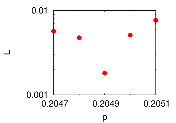
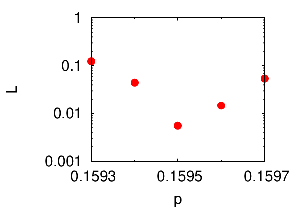
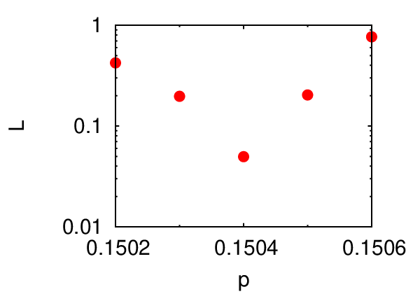
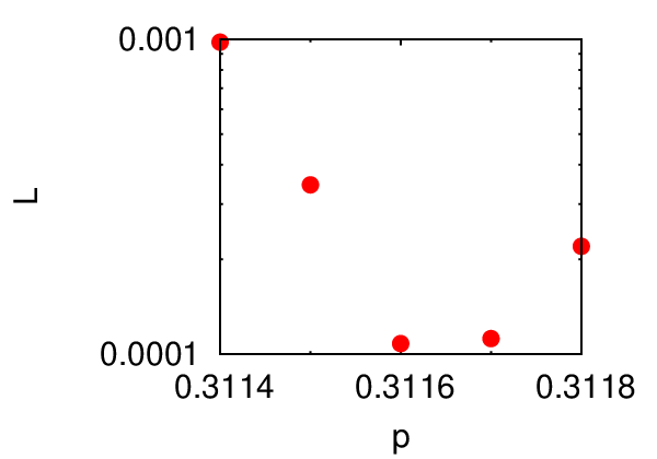
As it was mentioned in the Introduction, the results of computer simulations rather rarely reproduce a single common point of curves unless the number of prepared lattices is very high. It means, that finding the common point of curves for various linear system sizes may be quite problematic. In order to illustrate better this situation, we plot dependencies near with sites occupation probability step (see Fig. 3). And indeed, except for 4NN+2NN+NN neighborhood, the curves for various pairs of intersect at different points. Moreover, for the smallest values of the dependencies do not even increase monotonically with . At the same time, the dependencies prepared with the same accuracy exhibit single and sharp minimum (it is worth to mention, that values of are presented with the use of logarithmic scale). The minimum of corresponds to the percolation threshold . The estimated thresholds are presented in Tab. 1.
The plots presented in Fig. 3 make possible to detrmine the length of interval where the true value of percolation threshold is located. This length is equal to . Assuming that a real percolation threshold value is uniformly distributed in this interval one may evaluate the percolation threshold uncertainty as . The approach based on dependence gives evaluation of twice smaller and consequently . On the other hand the method of estimation based solely on dependencies, applied for similar neighborhood geometries leads to twice smaller lengths and consequently similar uncertainties but for ten times larger sampling () [45]. One can conclude, that the method used by Bastas et al. leads to reaching uncertainty of the percolation threshold value similar to those obtained with classical method but ten times faster.
Note, that an SC lattice with 4NN neighbors may be mapped onto two independent interpenetrated SC lattices but with two times larger lattice constant. Thus we expect the percolation threshold for the next-next-next-next-nearest neighbors to be equal exactly to . Indeed, the obtained value of 0.31160 agrees very well with values of percolation threshold estimated for the nearest neighbors obtained very recently in extensive Monte Carlo simulation [51] and its earlier estimations [52, *Lorenz1998, *Ballesteros1999, *PhysRevE.72.016126, *PhysRevE.87.052107, *Naeem1998, *Acharyya1998, *Grassberger1992].
Note, however, that reaching such accuracy requires, for , sampling over lattices realization [51], while we recovered the first five digits of with statistics lower by more than four orders of magnitude.
Knowing percolation threshold may be practically useful for many systems with neighborhoods ranging beyond nearest neighbors [60, *Vandermeer, *Chen, *Bianconi, *Yiu, *Smits, *Wang, *Kriel, *Rodrigues] or next-nearest neighbors [69, *Albert, *Boer]. Thus practical application of values for longer ranges of interaction among systems’ items cannot be generally excluded in all typical applications of the percolation theory, i.e. physics, chemistry, biology and social sciences.
Acknowledgements.
The work was supported by the Polish Ministry of Science and Higher Education and its grants for scientific research and PL-Grid infrastructure.References
- [1] D. Stauffer and A. Aharony, Introduction to Percolation Theory, 2nd ed. (Taylor and Francis, London, 1994).
- [2] B. Bollobás and O. Riordan, Percolation (Cambridge UP, Cambridge, 2006).
- [3] H. Kesten, Percolation Theory for Mathematicians (Brikhauser, Boston, 1982).
- [4] M. Sahimi, Applications of Percolation Theory (Taylor and Francis, London, 1994).
- [5] S. R. Broadbent and J. M. Hammersley, Mathematical Proceedings of the Cambridge Philosophical Society 53, 629 (1957).
- [6] H. Frisch, V. Vyssotsky, E. Sonnenblick, and J. Hammersley, Phys. Rev. 124, 1021 (1961).
- [7] H. L. Frisch, J. M. Hammersley, and D. J. A. Welsh, Phys. Rev. 126, 949 (1962).
- [8] K. Hoppe and G. J. Rodgers, Phys. Rev. E 90, 012815 (2014).
- [9] J. Wierman, D. Naor, and R. Cheng, Phys. Rev. E 72, 066116 (2005).
- [10] A. Rosowsky, Eur. Phys. J. B 15, 77 (2000).
- [11] D. Gaunt and M. Sykes, J. Phys. A: Math. Gen. 16, 783 (1983).
- [12] M. Sykes and M. Glen, J. Phys. A: Math. Gen. 9, 87 (1976).
- [13] M. Sykes, D. Gaunt, and M. Glen, J. Phys. A: Math. Gen. 9, 97 (1976a).
- [14] M. Sykes, D. Gaunt, and M. Glen, J. Phys. A: Math. Gen. 9, 715 (1976b).
- [15] M. Sykes, D. Gaunt, and M. Glen, J. Phys. A: Math. Gen. 9, 725 (1976c).
- [16] D. Gaunt and M. Sykes, J. Phys. A: Math. Gen. 9, 1109 (1976).
- [17] J. P. Clancy, A. Lupascu, H. Gretarsson, Z. Islam, Y. F. Hu, D. Casa, C. S. Nelson, S. C. LaMarra, G. Cao, and Y.-J. Kim, Phys. Rev. B 89, 054409 (2014).
- [18] J. Silva, R. Simoes, S. Lanceros-Mendez, and R. Vaia, EPL 93, 37005 (2011).
- [19] P. R. Shearing, D. J. L. Brett, and N. P. Brandon, Int. Mater. Rev. 55, 347 (2010).
- [20] B. I. Halperin and D. J. Bergman, Physica B 405, 2908 (2010).
- [21] S. C. Mun, M. Kim, K. Prakashan, H. J. Jung, Y. Son, and O. O. Park, Carbon 67, 64 (2014).
- [22] Y. Amiaz, S. Sorek, Y. Enzel, and O. Dahan, Water Resour. Res. 47, W10513 (2011).
- [23] S. F. Bolandtaba and A. Skauge, Transp. Porous Media 89, 357 (2011).
- [24] V. V. Mourzenko, J. F. Thovert, and P. M. Adler, Phys. Rev. E 84, 036307 (2011).
- [25] S. R. Abades, A. Gaxiola, and P. A. Marquet, J. Ecology 102, 1386 (2014).
- [26] G. Camelo-Neto and S. Coutinho, J. Stat. Mech.-Theory Exp. 2011, P06018 (2011).
- [27] N. Guisoni, E. S. Loscar, and E. V. Albano, Phys. Rev. E 83, 011125 (2011).
- [28] A. Simeoni, P. Salinesi, and F. Morandini, Int. J. Wildland Fire 20, 625 (2011).
- [29] K. Malarz, S. Kaczanowska, and K. Kulakowski, Int. J. Mod. Phys. C 13, 1017 (2002).
- [30] J. Silverberg, A. Barrett, M. Das, P. Petersen, L. Bonassar, and I. Cohen, Biophys. J. 107, 1721 (2014).
- [31] S. U. Suzuki and A. Sasaki, J. Theor. Biol. 276, 117 (2011).
- [32] J. Lindquist, J. Ma, P. van den Driessche, and F. H. Willeboordse, J. Math. Biol. 62, 143 (2011).
- [33] E. N. Naumova, J. Gorski, and Y. N. Naumov, Ann. Zool. Fenn. 45, 369 (2008).
- [34] W. Floyd, L. Kay, and M. Shapiro, Bull. Math. Biol. 70, 713 (2008).
- [35] T. Chandrashekar, C. M. Busch, Sci. Rep. 4, 6583 (2014).
- [36] M. E. Fisher, in Critical Phenomena, edited by M. S. Green (Academic Press, London, 1971) p. 1.
- [37] V. Privman, in Finite size scaling and numerical simulation of statistical systems, edited by V. Privman (World Scientific, Singapore, 1990) p. 1.
- [38] K. Binder, in Computational Methods in Field Theory, edited by C. B. Lang and H. Gausterer (Springer, Berlin, 1992).
- [39] D. P. Landau and K. Binder, A Guide to Monte Carlo Simulations in Statistical Physics, 2nd ed. (Cambridge UP, Cambridge, 2005).
- [40] N. Bastas, K. Kosmidis, and P. Argyrakis, Phys. Rev. E 84, 066112 (2011).
- [41] N. Bastas, K. Kosmidis, P. Giazitzidis, and M. Maragakis, “Method for estimating critical exponents in percolation processes with low sampling,” (2014), arXiv:1411.5834 [cond-mat.stat-mech] .
- [42] K. Malarz and S. Galam, Phys. Rev. E 71, 016125 (2005).
- [43] S. Galam and K. Malarz, Phys. Rev. E 72, 027103 (2005).
- [44] M. Majewski and K. Malarz, Acta Phys. Pol. B 38, 2191 (2007).
- [45] Ł. Kurzawski and K. Malarz, Rep. Math. Phys. 70, 163 (2012).
- [46] The detailed studies of properties and its scaling function but for a square lattice are given in Ref. [47].
- [47] M. Newman and R. Ziff, Phys. Rev. E 64, 016706 (2001).
- [48] J. Hoshen and R. Kopelman, Phys. Rev. B 14, 3438 (1976).
- [49] P. L. Leath, Phys. Rev. Lett. 36, 921 (1976).
- [50] I. V. Torin, Int. J. Mod. Phys. C 25, 1450064 (2014).
- [51] X. Xu, J. Wang, J.-P. Lv, and Y. Deng, Front. Phys. 9, 113 (2014).
- [52] J. Škvor and I. Nezbeda, Phys. Rev. E 79, 041141 (2009).
- [53] C. D. Lorenz and R. M. Ziff, J. Phys. A: Math. Gen. 31, 8147 (1998).
- [54] H. G. Ballesteros, L. A. Fernández, V. Martín-Mayor, A. M. noz Sudupe, G. Parisi, and J. J. Ruiz-Lorenzo, J. Phys. A: Math. Gen. 32, 1 (1999).
- [55] Y. Deng and H. W. J. Blöte, Phys. Rev. E 72, 016126 (2005).
- [56] J. Wang, Z. Zhou, W. Zhang, T. M. Garoni, and Y. Deng, Phys. Rev. E 87, 052107 (2013).
- [57] N. Jan and D. Stauffer, Int. J. Mod. Phys. C 9, 341 (1998).
- [58] M. Acharyya and D. Stauffer, Int. J. Mod. Phys. C 9, 643 (1998).
- [59] P. Grassberger, J. Phys. A: Math. Gen. 25, 5867 (1992).
- [60] A. Y. Birenbaum and C. Ederer, Phys. Rev. B 90, 214109 (2014).
- [61] J. Vandermeer, I. Perfecto, and N. Schellhorn, Landscape Ecol. 25, 509 (2010).
- [62] Y. Chen and C. A. Schuh, Phys. Rev. E 80, 040103 (2009).
- [63] G. Bianconi, EPL 101, 26003 (2013).
- [64] Y. Yiu, P. Bonfá, S. Sanna, R. De Renzi, P. Carretta, M. A. McGuire, A. Huq, and S. E. Nagler, Phys. Rev. B 90, 064515 (2014).
- [65] R. G. Smits, G. J. M. Koper, and M. Mandel, J. Phys. Chem. 97, 5745 (1993).
- [66] R. Wang, Y. Zhang, and C. Zhang, Results in Physics 4, 44 (2014).
- [67] J. N. Kriel, C. Karrasch, and S. Kehrein, Phys. Rev. B 90, 125106 (2014).
- [68] N. T. Rodrigues and T. J. Oliveira, J. Phys. A: Math. Theor. 47, 405002 (2014).
- [69] X. Gratens, A. Paduan-Filho, V. Bindilatti, N. F. Oliveira, Jr., and Y. Shapira, Phys. Rev. B 75, 184405 (2007).
- [70] M. V. Albert, A. Schnabel, and D. J. Field, PLoS Comput. Biol. 4, e000137 (2008).
- [71] M. M. Boer, P. Johnston, and R. J. Sadler, Ecol. Complex. 8, 347 (2011).