跳到论文正文
W Papers独立论文阅读器 arXiv:1501.01531 论文正文 计算阅读时间 · 0%
引用这篇论文根据当前论文元数据生成,正式投稿前建议核对。


License: arXiv.org perpetual non-exclusive license
arXiv:1501.01531v2 [math.DS] 07 Apr 2015

Non-standard real-analytic realizations of some rotations of the circle

Shilpak Banerjee
Abstract

We extend some aspects of the smooth approximation by conjugation method to the real-analytic set-up and create examples of zero entropy, uniquely ergodic real-analytic diffeomorphisms of the two dimensional torus metrically isomorphic to some (Liouvillian) irrational rotations of the circle.

1 Introduction

A smooth (C∞C^{\infty}) diffeomorphism ff of a compact manifold MM preserving a smooth measure mm is said to be a smooth realization of an abstract system (X,T,ν)(X,T,\nu) if there exists a metric isomorphism between the two systems. This problem of smooth realization remains stubbornly intractable in general, despite the fact that after assuming finiteness of the measure theoretic entropy of the system (X,T,ν)(X,T,\nu) and in some cases large (>2>2) dimension of MM, there is no known restriction for (X,T,ν)(X,T,\nu) to be realized as a smooth dynamical system on MM. See section 7.2 in [5] for a detailed discussion of this question.

Several variants of the smooth realization problem described above exists and in this paper we are interested in a particular case, namely the problem of non-standard realization in the real-analytic set-up. The problem of non-standard realization starts with a diffeomorphism gg of a compact manifold NN preserving a smooth measure ν\nu and seeks out a diffeomorphism ff of a compact manifold MM preserving a smooth measure mm such that the two systems are metrically isomorphic but not smoothly isomorphic. In this case we say that ff is a non-standard realization of gg on the manifold MM.

The earliest examples of non-standard realization appears in [1] where D.V. Anosov and A. Katok developed a scheme known as the approximation by conjugation method. They used this scheme to produce examples of non-standard realization of some irrational rotations of the circle as an ergodic smooth diffeomorphism of any manifold MM preserving a smooth measure mm provided the manifold admits an effective smooth action of the circle by mm-preserving smooth diffeomorphisms. The diffeomorphisms constructed in [1] realized circle rotations with Liouvillan rotation numbers. However it was not clear from this construction which Liouvillian rotations were realized. Later B. Fayad, M. Saprykina and A. Windsor extended this result in [6] and proved that any Liouvillian rotation of the circle can be realized. Moreover they also proved that if MM is a finite dimensional torus, then this realization can be made uniquely ergodic. Proving unique ergodicity using this technique brings out another aspect of this theory since one needs to retain control over every orbit as opposed to almost every orbit.

Also it should be mentioned that in [1], examples of non-standard realization of some ergodic translations of any finite dimensional torus were produced on any manifold admitting an effective smooth action of the circle by mm-preserving diffeomorphisms. Recently, M. Benhenda in [7] expanded this result to the case of ergodic translations by vectors with one arbitrary Liouvillian coordinate on any finite dimensional torus.

To complete the history of the smooth realization problem and its variants, it should also be noted that recently M. Benhenda in [9] produced examples of smooth diffeomorphisms on the product of a circle with a Hilbert cube having perfect Kronecker sets as their spectrum.

In our paper we seek to use the approximation by conjugation method and find examples of real-analytic uniquely ergodic diffeomorphisms on the two dimensional torus that are metrically isomorphic to some irrational rotation of the circle. However requiring the diffemorphism to be real-analytic imposes some additional difficulties (see section 7.2 in [5]). One possible way to overcome such difficulties is to work in manifolds which have a large collection of real-analytic diffeomorphisms commuting with the circle action and their singularities are uniformly bounded away from a complex neighbourhood of the real domain. An example of such a construction appears in [8]. In our case we work in the torus and customize the approximation by conjugation scheme with a trick that appeared in [2]. The key idea is to use entire functions that approximate certain carefully chosen step functions.

Our main theorem can be stated as follows:

Theorem 1.1.

There exists uniquely ergodic real-analytic diffeomorphisms of the two dimensional torus 𝕋2\mathbb{T}^{2} preserving the Lebesgue measure that are metrically isomorphic to some irrational rotations of the circle.

In this article we produce a complete proof of the above theorem. However we would also like to point out that the result easily generalizes to a higher dimensional torus. In section 7, we outline a proof of the above theorem in the case of a torus of any dimension.

We would also like to point out that very recently P. Kunde has proved the existence of a Real-analytic weak mixing diffeomorphism preserving a measurable Riemannian metric in [10] using some of the techniques developed in this paper. This solves Problem 3.9 posed by R. Gunesch and A. Katok in [3].

2 Preliminaries

The purpose of this section is to introduce some notations, give a brief description of the topology of real-analytic diffeomorphisms and finally lay down the approximation by conjugation scheme customized for our problem.

Throughout this paper, we will denote the two dimensional torus by 𝕋2:=ℝ2/ℤ2\mathbb{T}^{2}:=\mathbb{R}^{2}/\mathbb{Z}^{2}. We will use μ\mu to denote the standard Lebesgue measure on 𝕋2\mathbb{T}^{2} and λ\lambda to denote the Lebesgue measure on the unit circle 𝕋1:=ℝ/ℤ\mathbb{T}^{1}:=\mathbb{R}/\mathbb{Z}.

The topology of real-analytic diffeomorphisms

We start this section by giving a description of the space of measure preserving real-analytic diffeomorphisms on 𝕋2\mathbb{T}^{2}.

Any real-analytic diffeomorphism on 𝕋2\mathbb{T}^{2} homotopic to the identity admits a lift to a map from ℝ2\mathbb{R}^{2} to ℝ2\mathbb{R}^{2} of the form F⁡(x1,x2)=(x1+f1​(x1,x2),x2+f2​(x1,x2))F(x_{1},x_{2})=(x_{1}+f_{1}(x_{1},x_{2}),x_{2}+f_{2}(x_{1},x_{2})), where fi:ℝ2→ℝ2f_{i}:\mathbb{R}^{2}\to\mathbb{R}^{2} is a ℤ2\mathbb{Z}^{2}-periodic real-analytic functions. Any real-analytic ℤ2\mathbb{Z}^{2}-periodic function on ℝ2\mathbb{R}^{2} can be extended as a complex analytic function using the natural embedding (x1,x2)↦(x1+i​y1,x2+i​y2)(x_{1},x_{2})\mapsto(x_{1}+iy_{1},x_{2}+iy_{2}) of ℝ2\mathbb{R}^{2} in ℂ2\mathbb{C}^{2}. For a fixed ρ>0\rho>0, let Ωρ:={(z1,z2)∈ℂ2:|Im​(z1)|<ρ​ and ​|Im​(z2)|<ρ}\Omega_{\rho}:=\{(z_{1},z_{2})\in\mathbb{C}^{2}:|\text{Im}(z_{1})|<\rho\text{ and }|\text{Im}(z_{2})|<\rho\} and for a function ff defined on this set, define ‖f‖ρ:=supΩρ|f⁡((z1,z2))|\|f\|_{\rho}:=\sup_{\Omega_{\rho}}|f((z_{1},z_{2}))|. We define Cρω​(𝕋2)C^{\omega}_{\rho}(\mathbb{T}^{2}) to be the space of all ℤ2\mathbb{Z}^{2}-periodic real-analytic functions on ℝ2\mathbb{R}^{2} that extends to a holomorphic function on Ωρ\Omega_{\rho} and ‖f‖ρ<∞\|f\|_{\rho}<\infty.

Now we define, Diff ρω​(𝕋2,μ)\text{Diff }^{\omega}_{\rho}(\mathbb{T}^{2},\mu) to be the set of all measure preserving real-analytic diffeomorphisms of 𝕋2\mathbb{T}^{2} homotopic to the identity, whose lift FF to ℝ2\mathbb{R}^{2} satisfies fi∈Cρω​(𝕋2)f_{i}\in C^{\omega}_{\rho}(\mathbb{T}^{2}).

The metric in Diff ρω​(𝕋2,μ)\text{Diff }^{\omega}_{\rho}(\mathbb{T}^{2},\mu) is defined by

dρ​(F,G)=maxi=1,2⁡{infn∈ℤ‖fi−gi+n‖ρ}\displaystyle d_{\rho}(F,G)=\max_{i=1,2}\{\inf_{n\in\mathbb{Z}}\|f_{i}-g_{i}+n\|_{\rho}\}

Let (F1,F2)(F_{1},F_{2}) be the lift of a diffeomorphism F∈Diff ρω​(𝕋2,μ)F\in\text{Diff }^{\omega}_{\rho}(\mathbb{T}^{2},\mu), we define

‖D​F‖ρ:=maxi=1,2j=1,2⁡‖∂Fi∂xi‖ρ\displaystyle\|DF\|_{\rho}:=\max_{\begin{subarray}{c}i=1,2\\ j=1,2\end{subarray}}\Big\|\frac{\partial F_{i}}{\partial x_{i}}\Big\|_{\rho}

This completes the description of the analytic topology necessary for our construction. Also throughout this paper, the word “diffeomorphism” will refer to a real-analytic diffeomorphism. Also, the word “analytic topology” will refer to the topology of Diff ρω​(𝕋2,μ)\text{Diff }^{\omega}_{\rho}(\mathbb{T}^{2},\mu) described above. See [4] for a more extensive treatment of these spaces.

The approximation by conjugation scheme

Next in this section, we give a brief description of the approximation by conjugation scheme tailored for our purpose. This scheme was introduced in [1]. For a relatively upto date description of this scheme and its usefulness, one might refer to [5].

We start with ϕ\phi, a measure preserving 𝕋1\mathbb{T}^{1} action on the torus 𝕋2:=ℝ2/ℤ2\mathbb{T}^{2}:=\mathbb{R}^{2}/\mathbb{Z}^{2} defined as follows:

ϕt​((x1,x2))=(x1+t,x2)\displaystyle\phi^{t}\big((x_{1},x_{2})\big)=(x_{1}+t,x_{2})

The required measure preserving ergodic diffeomorphism TT is going to be constructed as a limit of periodic measure preserving diffeomorphisms TnT_{n} in the analytic topology described above. The diffeomorphisms TnT_{n} are defined by

Tn:=Hn−1∘ϕαn∘Hn\displaystyle T_{n}:=H_{n}^{-1}\circ\phi^{\alpha_{n}}\circ H_{n}

where αn∈ℚ∩[0,1)\alpha_{n}\in\mathbb{Q}\cap[0,1) and Hn∈Diff ρω​(𝕋2)H_{n}\in\text{Diff }^{\omega}_{\rho}(\mathbb{T}^{2}). The diffeomorphisms HnH_{n} and the rationals αn\alpha_{n} s are constructed inductively. Given HnH_{n} and αn\alpha_{n}, we construct at the n+1n+1 th stage, a diffeomorphism hn+1∈Diff ρω​(𝕋2)h_{n+1}\in\text{Diff }^{\omega}_{\rho}(\mathbb{T}^{2}) and define:

Hn+1=hn+1∘Hn\displaystyle H_{n+1}=h_{n+1}\circ H_{n}

αn+1\alpha_{n+1} is then defined and we would require it to be extremely close to αn\alpha_{n} in order to ensure the convergence of our construction.

The construction of hnh_{n} to suit our purpose is done in section 4. At each stage we ensure that TnT_{n} satisfies a finite version of the conjugacy that we would need eventually to conclude existence of the required metric isomorphism for the limit diffeomorphism. The measure theoretic result we require in that direction appears in section 3.

3 A measure theoretic lemma

In this section, our goal is to prove an abstract lemma from measure theory which is a slight generalization of Lemma 4.1 in [1].

First we recall a few definitions. A sequence of partitions {𝒫n}n\{\mathcal{P}_{n}\}_{n} of a Lebesgue space11 1 Also known as a standard probability space or a Lebesgue-Rokhlin space. We consider those spaces which are isomorphic mod 00 to the unit interval with the usual Lebesgue measure. (M,μ)(M,\mu) is called generating if there exists a measurable subset M′M^{\prime} of full measure such that {x}=∩n=1∞𝒫n(x)∀x∈M′\{x\}=\cap_{n=1}^{\infty}\mathcal{P}_{n}(x)\;\;\forall x\in M^{\prime}. We say that the sequence {𝒫n}n\{\mathcal{P}_{n}\}_{n} is monotonic if 𝒫n+1\mathcal{P}_{n+1} is a refinement of 𝒫n\mathcal{P}_{n}.

Lemma 4.1 from [1] gave us an easily checkable finite version of the conjugacy that one can use to prove the existence of a metric isomorphism of the limiting diffeomorphisms. Since the generating partitions used in the C∞C^{\infty} non-standard realization problem can easily made to be monotonic, this Lemma was sufficient. But in the real-analytic case, our construction is not flexible enough to guarantee monotonicity, so we need a modified version. Let us recall Lemma 4.1 from [1] since we will need it for our version.

Lemma 3.1.

Let {M(i),μ(i)},i=1,2\{M^{(i)},\mu^{(i)}\},\;i=1,2 be two Lebesgue spaces. Let 𝒫n(i)\mathcal{P}_{n}^{(i)} be a monotonic sequences of generating finite partitions of M(i)M^{(i)}. Let Tn(i)T_{n}^{(i)} be a sequence of automorphisms of M(i)M^{(i)} satisfying Tn(i)​𝒫n(i)=𝒫n(i)T_{n}^{(i)}\mathcal{P}_{n}^{(i)}=\mathcal{P}_{n}^{(i)} and suppose limn→∞Tn(i)=T(i)\lim_{n\to\infty}T_{n}^{(i)}=T^{(i)} weakly. Suppose ∃\exists metric isomorphisms Kn:M(1)/𝒫n(1)→M(2)/𝒫n(2)K_{n}:M^{(1)}/\mathcal{P}_{n}^{(1)}\to M^{(2)}/\mathcal{P}_{n}^{(2)} satisfying:

Kn−1​Tn(2)|𝒫n(2)​Kn=Tn(1)|𝒫n(1)\displaystyle K_{n}^{-1}T_{n}^{(2)}|_{\mathcal{P}_{n}^{(2)}}K_{n}=T_{n}^{(1)}|_{\mathcal{P}_{n}^{(1)}} (3.2)
Kn+1​(𝒫n(1))=Kn​(𝒫n(1))\displaystyle K_{n+1}(\mathcal{P}_{n}^{(1)})=K_{n}(\mathcal{P}_{n}^{(1)}) (3.3)

Then the automorphisms T(1)T^{(1)} and T(2)T^{(2)} are metrically isomorphic.

We would also like to point out at this point of time that KK in the proof was defined to be

K(x):=∩n=1∞Kn(Pn(1)(x))a.e.x∈M(1)\displaystyle K(x):=\cap_{n=1}^{\infty}K_{n}(P_{n}^{(1)}(x))\qquad\text{a.e.}\;\;x\in M^{(1)} (3.4)

Now we prove this variation which will allow us to accommodate a marginal “twist” that will appear in our construction.

Lemma 3.5.

Let {M(i),μ(i)},i=1,2\{M^{(i)},\mu^{(i)}\},\;i=1,2 be two Lebesgue spaces and let 𝒫n(1)\mathcal{P}_{n}^{(1)}. Let 𝒫n(i)\mathcal{P}_{n}^{(i)} be a sequence of generating finite partitions of M(i)M^{(i)}. Let {εn}\{\varepsilon_{n}\} be a sequence of positive numbers satisfying ∑n=1∞εn<∞\sum_{n=1}^{\infty}\varepsilon_{n}<\infty. In addition, assume that there exists a sequence of sets {En(i)}\{E_{n}^{(i)}\} in M(i)M^{(i)} satisfying:

μ(1)​(En(1))=μ(2)​(En(2))<εn\displaystyle\mu^{(1)}(E_{n}^{(1)})=\mu^{(2)}(E_{n}^{(2)})<\varepsilon_{n} (3.6)
Pn+1(1)​(x)∖En+1(1)⊂Pn(1)​(x)∀x∈M(1)∖En+1(1)\displaystyle P_{n+1}^{(1)}(x)\setminus E_{n+1}^{(1)}\subset P_{n}^{(1)}(x)\quad\forall\;x\in M^{(1)}\setminus E_{n+1}^{(1)} (3.7)
Pn+1(2)​(y)⊂Pn(2)​(y)∀y∈M(2)\displaystyle P_{n+1}^{(2)}(y)\subset P_{n}^{(2)}(y)\quad\forall\;y\in M^{(2)} (3.8)

Let Tn(1)T_{n}^{(1)} and Tn(2)T_{n}^{(2)} be two sequences of automorphisms of the spaces M(1)M^{(1)} and M(2)M^{(2)} satisfying:

Tn(i)​𝒫n(i)=𝒫n(i)i=1,2\displaystyle T_{n}^{(i)}\mathcal{P}_{n}^{(i)}=\mathcal{P}_{n}^{(i)}\quad\quad i=1,2 (3.9)
limn→∞Tn(i)=T(i)i=1,2\displaystyle\lim_{n\to\infty}T_{n}^{(i)}=T^{(i)}\quad\quad i=1,2 (3.10)
Tn(i)(∪m=n∞Em(i))=∪m=n∞Em(i)i=1,2\displaystyle T_{n}^{(i)}(\cup_{m=n}^{\infty}E_{m}^{(i)})=\cup_{m=n}^{\infty}E_{m}^{(i)}\quad\quad i=1,2 (3.11)

Note that the limit in 3.10 is taken in the weak topology. Suppose additionally there exists a sequence of metric isomorphisms Kn:M(1)/𝒫n(1)→M(2)/𝒫n(2)K_{n}:M^{(1)}/\mathcal{P}_{n}^{(1)}\to M^{(2)}/\mathcal{P}_{n}^{(2)} satisfying:

Kn−1​Tn(2)|𝒫n(2)​Kn=Tn(1)|𝒫n(1)\displaystyle K_{n}^{-1}T_{n}^{(2)}|_{\mathcal{P}_{n}^{(2)}}K_{n}=T_{n}^{(1)}|_{\mathcal{P}_{n}^{(1)}} (3.12)
Kn+1​(𝒫n+1(1)​(x))⊂Kn​(𝒫n(1)​(x))∀x∈M(1)∖En+1(1)\displaystyle K_{n+1}(\mathcal{P}_{n+1}^{(1)}(x))\subset K_{n}(\mathcal{P}_{n}^{(1)}(x))\quad\forall\;x\in M^{(1)}\setminus E_{n+1}^{(1)} (3.13)

Then the automorphisms T(1)T^{(1)} and T(2)T^{(2)} are metrically isomorphic.

Proof.

Put F(i)N:=∪n=N∞En(i)F^{(i)}_{N}:=\cup_{n=N}^{\infty}E_{n}^{(i)}. Consider the sequence of Lebesgue spaces MN(i):=M(i)∖FN(i)M^{(i)}_{N}:=M^{(i)}\setminus F^{(i)}_{N}.

Claim 1: ∃\exists a metric isomorphism K(N):MN(1)→MN(2)K_{(N)}:M^{(1)}_{N}\to M^{(2)}_{N}, satisfying K(N)−1​T(2)|MN(2)​K(N)=T(1)|MN(1)K_{(N)}^{-1}T^{(2)}|_{M_{N}^{(2)}}K_{(N)}=T^{(1)}|_{M_{N}^{(1)}}.

We define 𝒫N,k(i)\mathcal{P}^{(i)}_{N,k}, a finite measurable partition of MN(i)M^{(i)}_{N} by 𝒫N,k(i)​(x):=𝒫N+k(i)​(x)∖FN(i)\mathcal{P}^{(i)}_{N,k}(x):=\mathcal{P}^{(i)}_{N+k}(x)\setminus F^{(i)}_{N}. We note that the sequence of partition {𝒫N,k(i)}k\{\mathcal{P}^{(i)}_{N,k}\}_{k} is generating because {𝒫k(i)}k\{\mathcal{P}^{(i)}_{k}\}_{k} is generating. Additionally, condition 3.7 makes {𝒫N,k(i)}k\{\mathcal{P}^{(i)}_{N,k}\}_{k} a monotonic sequence of partition. We define KN,k​(𝒫N,k(1)​(x)):=KN+k​(𝒫N+k(1)​(x))∖FN(2)K_{N,k}(\mathcal{P}^{(1)}_{N,k}(x)):=K_{N+k}(\mathcal{P}^{(1)}_{N+k}(x))\setminus F^{(2)}_{N}. With this definition we claim that KN,k+1​(𝒫N,k(1)​(x))=KN,k​(𝒫N,k(1)​(x))K_{N,k+1}(\mathcal{P}^{(1)}_{N,k}(x))=K_{N,k}(\mathcal{P}^{(1)}_{N,k}(x)) ∀x∈MN(1)\forall x\in M^{(1)}_{N}. (Indeed, from 3.13 we get for a.e. x∈MN(1)x\in M^{(1)}_{N}, KN,k+1​(𝒫N,k+1(1)​(x))=KN+k+1​(𝒫N+k+1(1)​(x))∖FN(2)⊂KN+k​(𝒫N+k(1)​(x))∖FN(2)=KN,k​(𝒫N,k(1)​(x))K_{N,k+1}(\mathcal{P}^{(1)}_{N,k+1}(x))=K_{N+k+1}(\mathcal{P}^{(1)}_{N+k+1}(x))\setminus F^{(2)}_{N}\subset K_{N+k}(\mathcal{P}^{(1)}_{N+k}(x))\setminus F^{(2)}_{N}=K_{N,k}(\mathcal{P}^{(1)}_{N,k}(x)). This with the fact that KN,k+1​(𝒫N,k+1(1)​(x))∈𝒫N,k+1(2)K_{N,k+1}(\mathcal{P}^{(1)}_{N,k+1}(x))\in\mathcal{P}^{(2)}_{N,k+1} and {𝒫N,k(2)}k\{\mathcal{P}^{(2)}_{N,k}\}_{k} is a monotonic sequence of partitions helps us in concluding the claim). Observe that 3.9, 3.11 and 3.12 guarantees that KN,k−1​TN+k(2)|𝒫N,k(2)​KN,k=TN+k(1)|𝒫N,k(1)K_{N,k}^{-1}T_{N+k}^{(2)}|_{\mathcal{P}_{N,k}^{(2)}}K_{N,k}=T_{N+k}^{(1)}|_{\mathcal{P}_{N,k}^{(1)}}. So we can apply Lemma 3.1 to guarantee the existence of a metric isomorphism K(N):MN(1)→MN(2)K_{(N)}:M^{(1)}_{N}\to M^{(2)}_{N} defined for a.e. x∈MN(1)x\in M^{(1)}_{N} by K(N)(x)=∩k=1∞KN,k(𝒫N,k(1)(x))K_{(N)}(x)=\cap^{\infty}_{k=1}K_{N,k}(\mathcal{P}^{(1)}_{N,k}(x)). This finishes claim 1.

Claim 2: K(N+1)​(x)=KN​(x)K_{(N+1)}(x)=K_{N}(x) for a.e. x∈MN(1)x\in M^{(1)}_{N}

Follows from the definition of K(N)K_{(N)}. Indeed, note that K(N+1)(x)=∩k=1∞KN+1,k(𝒫N+1,k(1)(x))=∩k=1∞KN+k+1(𝒫N+k+1(1)(x))∖FN+1(2)=∩k=0∞KN+k+1(𝒫N+k+1(1)(x))∖FN+1(2)K_{(N+1)}(x)=\cap^{\infty}_{k=1}K_{N+1,k}(\mathcal{P}^{(1)}_{N+1,k}(x))=\cap^{\infty}_{k=1}K_{N+k+1}(\mathcal{P}^{(1)}_{N+k+1}(x))\setminus F^{(2)}_{N+1}=\cap^{\infty}_{k=0}K_{N+k+1}(\mathcal{P}^{(1)}_{N+k+1}(x))\setminus F^{(2)}_{N+1}. The last equality follows from 3.13.

Claim 3: There exists a metric isomorphism K:M(1)→M(2)K:M^{(1)}\to M^{(2)} satisfying K−1​T(2)​K=T(1)K^{-1}T^{(2)}K=T^{(1)}

Note that condition 3.6 implies that a.e. x∈En(1)x\in E_{n}^{(1)} for at most finitely many nn. Indeed, if E={x:x∈En​ for infinitely many ​n}E=\{x:x\in E_{n}\text{ for infinitely many }n\}, then E⊂∩n=m∞En∀mE\subset\cap_{n=m}^{\infty}E_{n}\;\forall\;m and limm→∞μ(1)(∩n=m∞En)=0\lim_{m\to\infty}\mu^{(1)}(\cap_{n=m}^{\infty}E_{n})=0. So we can define for a.e. x∈M(1)x\in M^{(1)}, K​(x):=K(N)​(x)K(x):=K_{(N)}(x) if x∈MN(1)x\in M^{(1)}_{N}. Now claim 3 easily follows from claim 2. ∎

4 Construction of hn+1h_{n+1} and the conjugating analytic diffeomorphism

As mentioned earlier, the construction in an inductive process so we assume that we have already defined h1,…,hn∈ Diff ρω​(𝕋2)h_{1},\ldots,h_{n}\in\text{ Diff }^{\omega}_{\rho}(\mathbb{T}^{2}), two sequences of integers {km}m=0n−1\{k_{m}\}_{m=0}^{n-1} and {lm}m=0n−1\{l_{m}\}_{m=0}^{n-1} and a sequence of rational numbers {αm}m=1n\{\alpha_{m}\}_{m=1}^{n}. At the n+1n+1 th stage we construct hn+1∈ Diff ρω​(𝕋2)h_{n+1}\in\text{ Diff }^{\omega}_{\rho}(\mathbb{T}^{2}) as a composition of four different diffeomorphisms.

First, we let lnl_{n} to be a large enough integer so that in particular we have

ln>2n​‖D​Hn‖0\displaystyle l_{n}>2^{n}\|DH_{n}\|_{0} (4.1)

We will use this parameter to ensure that a sequence of partitions we construct later is generating.

At this point we continue with our construction by assuming knk_{n} to be any integer. Later we will impose more conditions on the largeness of knk_{n} (see 5.5) to ensure that αn+1\alpha_{n+1} is sufficiently close to αn\alpha_{n} which will be required to show the convergence of TnT_{n}. Largeness of {kn}\{k_{n}\} will also be during the proof of unique ergodicity of TT (see proof of proposition 6.2). So later we will choose knk_{n} to be larger than the maximum of these two requirements.

The key idea which we use here for constructing the diffeomorphism hn+1h_{n+1} is from [2]. We observe that using functions of the form (x1,x2)↦(x1+ψ~1​(x2),x2)(x_{1},x_{2})\mapsto(x_{1}+\tilde{\psi}_{1}(x_{2}),x_{2}) and (x1,x2)↦(x1,x2+ψ~2​(x1))(x_{1},x_{2})\mapsto(x_{1},x_{2}+\tilde{\psi}_{2}(x_{1})), where ψ~i\tilde{\psi}_{i}s are carefully chosen step functions, we can “break” a partition of 𝕋2\mathbb{T}^{2} which is permuted cyclically by ϕαn+1\phi^{\alpha_{n+1}} and reform it into a generating partition that is permuted cyclically by Tn+1T_{n+1}. One can imagine that this construction is similar to playing the sliding puzzle game called “mystic square” or “game of 15”.

Construction of a discontinuous version of the conjugating diffeomorphism

Refer to caption →h~1,n+1\xrightarrow{\tilde{h}_{1,n+1}} Refer to caption
→h~2,n+1\xrightarrow{\tilde{h}_{2,n+1}} Refer to caption →h~3,n+1\xrightarrow{\tilde{h}_{3,n+1}} Refer to caption
→h~4,n+1\xrightarrow{\tilde{h}_{4,n+1}} Refer to caption     Refer to caption
Figure 1: Illustration of the action of h~n+1\tilde{h}_{n+1} on three vertically stacked up atoms of 𝒢l,q\mathcal{G}_{l,q} and how it is transformed into three atoms of 𝒯q\mathcal{T}_{q} by h~n+1\tilde{h}_{n+1}. This diagram is drawn with qn=3q_{n}=3 and ln=3l_{n}=3. Note that the choice of knk_{n} and sns_{n} has not been used for this illustration since they do not alter the combinatorics in any way. Also one should note that the last map h~4,n+1\tilde{h}_{4,n+1} preserves the atoms of 𝒯q\mathcal{T}_{q}, so combinatorially it is unnecessary.

Here our goal is to construct a discontinuous map h~n+1:𝕋2→𝕋2\tilde{h}_{n+1}:\mathbb{T}^{2}\to\mathbb{T}^{2} which “breaks” down a partition of 𝕋2\mathbb{T}^{2} and rearranges it into a generating partition. Later in this section, we will see that we can approximate this function by real-analytic diffeomorphisms.

Let us consider the following three step functions:

ψ~1,n+1:[0,1)→ℝ\displaystyle\tilde{\psi}_{1,n+1}:[0,1)\to\mathbb{R} defined by ψ~1,n+1​(x)=∑i=1ln−1ln−iln2​qn​χ[iln,i+1ln]​(x)\displaystyle\tilde{\psi}_{1,n+1}(x)=\sum_{i=1}^{l_{n}-1}\frac{l_{n}-i}{l_{n}^{2}q_{n}}\chi_{[\frac{i}{l_{n}},\frac{i+1}{l_{n}}]}(x)
ψ~2,n+1:[0,1)→ℝ\displaystyle\tilde{\psi}_{2,n+1}:[0,1)\to\mathbb{R} defined by ψ~2,n+1​(x)=∑i=0ln2​qn−1(iln−⌊iln⌋)​χ[iln2​qn,i+1ln2​qn]​(x)\displaystyle\tilde{\psi}_{2,n+1}(x)=\sum_{i=0}^{l_{n}^{2}q_{n}-1}\biggl(\frac{i}{l_{n}}-\Big\lfloor\frac{i}{l_{n}}\Big\rfloor\biggr)\chi_{[\frac{i}{l_{n}^{2}q_{n}},\frac{i+1}{l_{n}^{2}q_{n}}]}(x)
ψ~3,n+1:[0,1)→ℝ\displaystyle\tilde{\psi}_{3,n+1}:[0,1)\to\mathbb{R} defined by ψ~3,n+1​(x)=∑i=0ln−1iln2​qn​χ[iln,i+1ln]​(x)\displaystyle\tilde{\psi}_{3,n+1}(x)=\sum_{i=0}^{l_{n}-1}\frac{i}{l_{n}^{2}q_{n}}\chi_{[\frac{i}{l_{n}},\frac{i+1}{l_{n}}]}(x) (4.2)

Now we are ready to define the required map h~n+1\tilde{h}_{n+1} as the composition of four different maps:

h~n+1:=h~4,n+1∘h~3,n+1∘h~2,n+1∘h~1,n+1\displaystyle\tilde{h}_{n+1}:=\tilde{h}_{4,n+1}\circ\tilde{h}_{3,n+1}\circ\tilde{h}_{2,n+1}\circ\tilde{h}_{1,n+1} (4.3)

Here the maps h~i,n+1:𝕋2→𝕋2\tilde{h}_{i,n+1}:\mathbb{T}^{2}\to\mathbb{T}^{2} for i=1,2,3i=1,2,3 and 44 are defined as follows:

h~1,n+1​((x1,x2))\displaystyle\tilde{h}_{1,n+1}((x_{1},x_{2})) =(x1+ψ~1,n+1​(x2)mod1,x2)\displaystyle=(x_{1}+\tilde{\psi}_{1,n+1}(x_{2})\mod 1\;,\;x_{2})
h~2,n+1​((x1,x2))\displaystyle\tilde{h}_{2,n+1}((x_{1},x_{2})) =(x1,x2+ψ~2,n+1​(x1)mod1)\displaystyle=(x_{1}\;,\;x_{2}+\tilde{\psi}_{2,n+1}(x_{1})\mod 1)
h~3,n+1​((x1,x2))\displaystyle\tilde{h}_{3,n+1}((x_{1},x_{2})) =(x1−ψ~3,n+1​(x2)mod1,x2)\displaystyle=(x_{1}-\tilde{\psi}_{3,n+1}(x_{2})\mod 1\;,\;x_{2})
h~4,n+1​((x1,x2))\displaystyle\tilde{h}_{4,n+1}((x_{1},x_{2})) :=(x1,x2+qn​x2mod1)\displaystyle:=(x_{1},\;x_{2}+q_{n}x_{2}\mod 1) (4.4)

In order to properly understand the action of h~n+1\tilde{h}_{n+1} on 𝕋2\mathbb{T}^{2}, we look at the following two partitions of 𝕋2\mathbb{T}^{2}:

𝒯q\displaystyle\mathcal{T}_{q} ={Δi,q:=[iq,i+1q)×[0,1):i=0,1,…,q−1}\displaystyle=\big\{\Delta_{i,q}:=[\frac{i}{q},\frac{i+1}{q})\times[0,1):i=0,1,\ldots,q-1\big\} (4.5)
𝒢l,q\displaystyle\mathcal{G}_{l,q} ={[il​q,i+1l​q)×[jl,j+1l):i=0,1,…lq−1,j=0,1,…l−1}\displaystyle=\big\{[\frac{i}{lq},\frac{i+1}{lq})\times[\frac{j}{l},\frac{j+1}{l}):i=0,1,\ldots lq-1,\;\;j=0,1,\ldots l-1\big\} (4.6)

Now the action of h~n+1−1\tilde{h}_{n+1}^{-1} is clear. Its job is to break the atoms of the partition 𝒯ln2​qn\mathcal{T}_{l_{n}^{2}q_{n}} into lnl_{n} pieces and rearrange those broken pieces into the atoms of the partition 𝒢ln,qn\mathcal{G}_{l_{n},q_{n}}. Note that the diameter of the atoms of partition 𝒢ln,qn\mathcal{G}_{l_{n},q_{n}} is bounded by a small number, namely 1l\frac{1}{l}. See figure 1 for an elementary demonstration of this combinatorics at work.

Of course h~n+1\tilde{h}_{n+1} is not analytic and in fact it is not even continuous, so we need to construct hn+1h_{n+1}, an entire diffeomorphism ‘close’ to h~n+1\tilde{h}_{n+1}. At this point we need to remind ourself that this will be possible because we can approximate step functions by real-analytic functions which extends holomorphically to the entire complex plane as an entire function. This hn+1h_{n+1} will somewhat successfully emulate the combinatorial picture produced by h~n+1\tilde{h}_{n+1} i.e. hn+1−1h_{n+1}^{-1} successfully compresses the bulk of the measure of an element of 𝒯qn+1\mathcal{T}_{q_{n+1}} into a set of small diameter but one needs to remember that there is an ‘error’ set (see 5.1) of small measure where we loose control.

Construction of the real-analytic conjugating diffeomorphism

Refer to caption Refer to caption Refer to caption Refer to caption
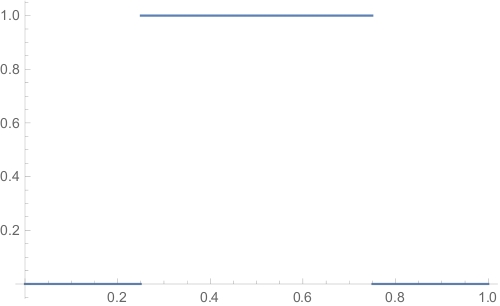
Figure 2: Illustration (using mathematica) of approximation of a step function χ[14,34]\chi_{[\frac{1}{4},\frac{3}{4}]} using the function ss. Here the first three pictures depict the function s⁡(x):=exp⁡(−exp⁡(−A⁡(x−14)))−exp⁡(−exp⁡(−A⁡(x−34)))s(x):=\exp(-\exp(-A(x-\frac{1}{4})))-\exp(-\exp(-A(x-\frac{3}{4}))) is depicted with A=10A=10, A=25A=25 and A=45A=45. We should also note that ss here is not periodic. In Lemma 4.7, we use an infinite sum of such functions to obtain periodicity.

We need the following lemma about approximation of step functions by real-analytic functions. This will allow us to construct an analytic hn+1h_{n+1} ‘close’ to the discontinuous map h~n+1\tilde{h}_{n+1} obtained by using step functions. The approximation used in the lemma is illustrated in Figure 2.

Lemma 4.7.

Let kk and NN be two positive integer and α=(α0,…,αk−1)∈[0,1)k\alpha=(\alpha_{0},\ldots,\alpha_{k-1})\in[0,1)^{k}. Consider a step function of the form

s~α,N:[0,1)→ℝ defined bys~α,N​(x)=∑i=0k​N−1α~i​χ[ik​N,i+1k​N)​(x)\displaystyle\tilde{s}_{\alpha,N}:[0,1)\to\mathbb{R}\quad\text{ defined by}\quad\tilde{s}_{\alpha,N}(x)=\sum_{i=0}^{kN-1}\tilde{\alpha}_{i}\chi_{[\frac{i}{kN},\frac{i+1}{kN})}(x)

Here α~i:=αj\tilde{\alpha}_{i}:=\alpha_{j} where j:=imodkj:=i\mod k. Then, given any ε>0\varepsilon>0 and δ>0\delta>0, there exists a 1N\frac{1}{N}-periodic entire function sα,N:ℝ→ℝs_{\alpha,N}:\mathbb{R}\to\mathbb{R} satisfying

supx∈[0,1)∖F|sα,N​(x)−s~α,N​(x)|<ε\displaystyle\sup_{x\in[0,1)\setminus F}|s_{\alpha,N}(x)-\tilde{s}_{\alpha,N}(x)|<\varepsilon (4.8)

Where F=∪i=0k​N−1Ii⊂[0,1)F=\cup_{i=0}^{kN-1}I_{i}\subset[0,1) is a union of intervals centred around ik​N,i=1,…,k​N−1\frac{i}{kN},\;i=1,\ldots,kN-1 and I0=[0,δ2​k​N]∪[1−δ2​k​N,1)I_{0}=[0,\frac{\delta}{2kN}]\cup[1-\frac{\delta}{2kN},1) and λ⁡(Ii)=δk​N​∀i\lambda(I_{i})=\frac{\delta}{kN}\;\forall\;i.

Proof.

We define the following function:

sα,N:ℝ→ℝ defined by\displaystyle s_{\alpha,N}:\mathbb{R}\to\mathbb{R}\quad\text{ defined by }
sα,N​(x)=∑n=−∞∞(∑i=0k−1αi​(e−e−A⁡(x−n​k+ik​N)−e−e−A⁡(x−n​k+i+1k​N)))\displaystyle s_{\alpha,N}(x)=\sum_{n=-\infty}^{\infty}\biggl(\sum_{i=0}^{k-1}\alpha_{i}\big(e^{-e^{-A(x-\frac{nk+i}{kN})}}-e^{-e^{-A(x-\frac{nk+i+1}{kN})}}\big)\biggr)

Note that sα,Ns_{\alpha,N} is a 1N\frac{1}{N}-periodic entire function defined on the real line. After choosing a large enough constant AA, we can guarantee that sα,Ns_{\alpha,N} satisfies condition 4.8. ∎

Now we are ready to produce an entire diffeomorphism ‘close’ to h~n+1\tilde{h}_{n+1}. First we use Lemma 4.7 to define three entire functions approximating the step functions defined above as follows:

ψ1,n+1:=sα(1),N(1)where α(1)0=0,α(1)i=ln−iln2​qn,i=1,…kn−1,N(1)=1;\displaystyle\psi_{1,n+1}:=s_{\alpha^{(1)},N^{(1)}}\;\text{where }\alpha^{(1)}_{0}=0,\;\alpha^{(1)}_{i}=\frac{l_{n}-i}{l_{n}^{2}q_{n}},\;i=1,\ldots k_{n}-1,\;N^{(1)}=1; (4.9)
ψ2,n+1:=sα(2),N(2)where α(2)i=iln,i=1,…ln−1,N(2)=lnqn;\displaystyle\psi_{2,n+1}:=s_{\alpha^{(2)},N^{(2)}}\;\text{where }\alpha^{(2)}_{i}=\frac{i}{l_{n}},\;i=1,\ldots l_{n}-1,\;N^{(2)}=l_{n}q_{n}; (4.10)
ψ3,n+1:=sα(3),N(3)where α(3)i=iln2​qn,i=1,…ln−1,N(3)=1;\displaystyle\psi_{3,n+1}:=s_{\alpha^{(3)},N^{(3)}}\;\text{where }\alpha^{(3)}_{i}=\frac{i}{l_{n}^{2}q_{n}},\;i=1,\ldots l_{n}-1,\;N^{(3)}=1; (4.11)

With the above definitions, and using 3​ε=δ=12ln2​qn​ln2​qn3\varepsilon=\delta=\frac{1}{2^{l_{n}^{2}q_{n}}l_{n}^{2}q_{n}} in Lemma 4.7, we can conclude that there exists three measurable sets Fi,n+1F_{i,n+1} for i=1,2,3i=1,2,3 such that:

supx∈[0,1)−F1,n|ψ1,n+1​(x)−ψ~1,n+1​(x)|<ελ⁡(F1,n)<12ln2​qn​ln2​qn\displaystyle\sup_{x\in[0,1)-F_{1,n}}|\psi_{1,n+1}(x)-\tilde{\psi}_{1,n+1}(x)|<\varepsilon\quad\quad\lambda(F_{1,n})<\frac{1}{2^{l_{n}^{2}q_{n}}l_{n}^{2}q_{n}} (4.12)
supx∈[0,1)−F2,n|ψ2,n+1​(x)−ψ~2,n+1​(x)|<ελ⁡(F2,n)<12ln2​qn​ln2​qn\displaystyle\sup_{x\in[0,1)-F_{2,n}}|\psi_{2,n+1}(x)-\tilde{\psi}_{2,n+1}(x)|<\varepsilon\quad\quad\lambda(F_{2,n})<\frac{1}{2^{l_{n}^{2}q_{n}}l_{n}^{2}q_{n}} (4.13)
supx∈[0,1)−F3,n|ψ3,n+1​(x)−ψ~3,n+1​(x)|<ελ⁡(F3,n)<12ln2​qn​ln2​qn\displaystyle\sup_{x\in[0,1)-F_{3,n}}|\psi_{3,n+1}(x)-\tilde{\psi}_{3,n+1}(x)|<\varepsilon\quad\quad\lambda(F_{3,n})<\frac{1}{2^{l_{n}^{2}q_{n}}l_{n}^{2}q_{n}} (4.14)

Additionally its important to notice at this point that ψ2,n+1\psi_{2,n+1} is 1qn\frac{1}{q_{n}} periodic.

Now we are ready to define hn+1h_{n+1} as the composition of four entire diffeomorphisms:

hn+1:=h4,n+1∘h3,n+1∘h2,n+1∘h1,n+1\displaystyle h_{n+1}:=h_{4,n+1}\circ h_{3,n+1}\circ h_{2,n+1}\circ h_{1,n+1} (4.15)

Here the diffeomorphisms hi,n+1:𝕋2→𝕋2h_{i,n+1}:\mathbb{T}^{2}\to\mathbb{T}^{2} for i=1,2,3i=1,2,3 and 44 are defined as follows:

h1,n+1​((x1,x2))\displaystyle h_{1,n+1}((x_{1},x_{2})) :=(x1+ψ1,n+1​(x2)mod1,x2)\displaystyle:=(x_{1}+\psi_{1,n+1}(x_{2})\mod 1\;,\;x_{2})
h2,n+1​((x1,x2))\displaystyle h_{2,n+1}((x_{1},x_{2})) :=(x1,x2+ψ2,n+1​(x1)mod1)\displaystyle:=(x_{1}\;,\;x_{2}+\psi_{2,n+1}(x_{1})\mod 1)
h3,n+1​((x1,x2))\displaystyle h_{3,n+1}((x_{1},x_{2})) :=(x1−ψ3,n+1​(x2)mod1,x2)\displaystyle:=(x_{1}-\psi_{3,n+1}(x_{2})\mod 1\;,\;x_{2})
h4,n+1​((x1,x2))\displaystyle h_{4,n+1}((x_{1},x_{2})) :=(x1,x2+qn​x2mod1)\displaystyle:=(x_{1},\;x_{2}+q_{n}x_{2}\mod 1) (4.16)

Note that it follows from the periodicity of ψi,n+1\psi_{i,n+1} (which was guaranteed by lemma 4.7):

hn+1∘ϕαn=ϕαn∘hn+1\displaystyle h_{n+1}\circ\phi^{\alpha_{n}}=\phi^{\alpha_{n}}\circ h_{n+1} (4.17)

We define our conjugating diffemorphism Hn+1H_{n+1} as follows:

Hn+1:=hn+1∘Hn\displaystyle H_{n+1}:=h_{n+1}\circ H_{n} (4.18)

This completes the construction of the conjugating diffeomorphism at the n+1n+1 th stage of the induction.

We end this section by defining,

qn+1:=kn​ln2​qn,pn+1:=kn​ln2​pn+1,αn+1:=pn+1qn+1\displaystyle q_{n+1}:=k_{n}l_{n}^{2}q_{n},\quad\quad p_{n+1}:=k_{n}l_{n}^{2}p_{n}+1,\quad\quad\alpha_{n+1}:=\frac{p_{n+1}}{q_{n+1}} (4.19)

Finally, we let

Tn+1:=Hn+1−1∘ϕαn+1∘Hn+1\displaystyle T_{n+1}:=H_{n+1}^{-1}\circ\phi^{\alpha_{n+1}}\circ H_{n+1} (4.20)
Remark.

Note that

Tn+1\displaystyle T_{n+1} =Hn+1−1∘ϕαn+1∘Hn+1\displaystyle=H_{n+1}^{-1}\circ\phi^{\alpha_{n+1}}\circ H_{n+1}
=h1,n+1−1∘h2,n+1−1∘h3,n+1−1∘h4,n+1−1∘ϕαn+1∘h4,n+1∘h3,n+1∘h2,n+1∘h1,n+1\displaystyle=h_{1,n+1}^{-1}\circ h_{2,n+1}^{-1}\circ h_{3,n+1}^{-1}\circ h_{4,n+1}^{-1}\circ\phi^{\alpha_{n+1}}\circ h_{4,n+1}\circ h_{3,n+1}\circ h_{2,n+1}\circ h_{1,n+1}
=h1,n+1−1∘h2,n+1−1∘ϕαn+1∘h2,n+1∘h1,n+1\displaystyle=h_{1,n+1}^{-1}\circ h_{2,n+1}^{-1}\circ\phi^{\alpha_{n+1}}\circ h_{2,n+1}\circ h_{1,n+1}

So h3,n+1h_{3,n+1} and h4,n+1h_{4,n+1} are redundant for the definition of Tn+1T_{n+1}, but h3,n+1h_{3,n+1} will later play an important role as a tool to “untwist” our construction albeit with an error. h4,n+1h_{4,n+1} will be crucial to ensure that this error set we would construct does not contain any whole orbit. This is important because we wish to conclude that our limiting diffeomorphism is uniquely ergodic and hence we do not wish to give up control over even a single orbit.

5 Existence of a limiting diffeomorphism conjugate to a rotation

The purpose of this section is to show that the sequence TnT_{n} defined in 4.20 connverges to some T∈Diff ρω​(𝕋2)T\in\text{Diff }^{\omega}_{\rho}(\mathbb{T}^{2}) for any ρ\rho. In fact this TT will be entire.

We define the error set Eqn+1⊂𝕋2E_{q_{n+1}}\subset\mathbb{T}^{2} as follows:

Hn+1​(Eqn+1):=Eqn+1(v)​⋃Eqn+1(d)\displaystyle H_{n+1}(E_{q_{n+1}}):=E_{q_{n+1}}^{(v)}\bigcup E_{q_{n+1}}^{(d)} (5.1)

Here

Eqn+1(v):=⋃i=0ln2​qn−1[iln2​qn−12ln2​qn​ln2​qn,iln2​qn+12ln2​qn​ln2​qn]×𝕋1\displaystyle E_{q_{n+1}}^{(v)}:=\bigcup_{i=0}^{l_{n}^{2}q_{n}-1}\Big[\frac{i}{l_{n}^{2}q_{n}}-\frac{1}{2^{l_{n}^{2}q_{n}}l_{n}^{2}q_{n}},\frac{i}{l_{n}^{2}q_{n}}+\frac{1}{2^{l_{n}^{2}q_{n}}l_{n}^{2}q_{n}}\Big]\times\mathbb{T}^{1}
Eqn+1(d)=h4,n+1​(⋃i=0ln−1𝕋1×[iln−12ln2​qn​ln2​qn,iln+12ln2​qn​ln2​qn])\displaystyle E_{q_{n+1}}^{(d)}=h_{4,n+1}\biggl(\bigcup_{i=0}^{l_{n}-1}\mathbb{T}^{1}\times\Big[\frac{i}{l_{n}}-\frac{1}{2^{l_{n}^{2}q_{n}}l_{n}^{2}q_{n}},\frac{i}{l_{n}}+\frac{1}{2^{l_{n}^{2}q_{n}}l_{n}^{2}q_{n}}\Big]\biggr)

Note that Eqn+1E_{q_{n+1}} is the set where we do not have any control. The darkened region of figure 33 represents how this error set is spread over 𝕋2\mathbb{T}^{2}.

Getting back to the proof, we define the following partition of 𝕋2\mathbb{T}^{2}:

ℱq:={Hn+1−1Δi,q:i=0,1,…,q−1}\displaystyle\mathcal{F}_{q}:=\{H_{n+1}^{-1}\Delta_{i,q}:i=0,1,\ldots,q-1\} (5.2)

We need the following proposition about some basic inclusions and estimates.

Refer to caption
Figure 3: The darkened region represents Hn+1​(Eqn+1)H_{n+1}(E_{q_{n+1}}) and the horizontal line represents a ϕt\phi^{t}-orbit. The diagram is made with qn=3q_{n}=3 and ln=3l_{n}=3. Note that the diagonal parts corresponds to Eqn+1(d)E^{(d)}_{q_{n+1}} and the vertical portion corresponds to Eqn+1(v)E^{(v)}_{q_{n+1}}.
Proposition 5.3.
(1)\displaystyle(1) μ⁡(Eqn+1)≤22ln2​qn\displaystyle\quad\mu(E_{q_{n+1}})\leq\frac{2}{2^{l_{n}^{2}q_{n}}}
(2)\displaystyle(2) ℱqn+1​(x)∖Eqn+1⊂ℱqn​(x)∀x∈𝕋2∖Eqn+1\displaystyle\quad\mathcal{F}_{q_{n+1}}(x)\setminus E_{q_{n+1}}\subset\mathcal{F}_{q_{n}}(x)\quad\forall\;x\in\mathbb{T}^{2}\setminus E_{q_{n+1}}
(3)\displaystyle(3) ℱqn→ε​ as ​n→∞(Here ​ε​ is the trivial partition into points).\displaystyle\quad\mathcal{F}_{q_{n}}\to\varepsilon\text{ as }n\to\infty\qquad(\text{Here }\varepsilon\text{ is the trivial partition into points}).
(4)\displaystyle(4) Tn​(ℱqn)=ℱqn\displaystyle\quad T_{n}\big(\mathcal{F}_{q_{n}}\big)=\mathcal{F}_{q_{n}}
Proof.

Statement (1) follows as a result of direct but obvious computation.

To conclude statement (2), first we note that F1,n×𝕋1⊂Eqn+1(v)F_{1,n}\times\mathbb{T}^{1}\subset E_{q_{n+1}}^{(v)}, 𝕋1×F2,n⊂h4,n+1−1​Eqn+1(d)\mathbb{T}^{1}\times F_{2,n}\subset h_{4,n+1}^{-1}E_{q_{n+1}}^{(d)} and F3,n×𝕋1⊂Eqn+1(v)F_{3,n}\times\mathbb{T}^{1}\subset E_{q_{n+1}}^{(v)} (see 4.12, 4.13 and 4.14). So, for any 0≤i<qn+10\leq i<q_{n+1}, i′=⌊iln2​qn⌋i^{\prime}=\lfloor\frac{i}{l_{n}^{2}q_{n}}\rfloor and j=⌊iqn⌋j=\lfloor\frac{i}{q_{n}}\rfloor, we have:

hn+1−1​(Δi′,ln2​qn∖Hn+1​(Eqn+1))⊂Δj,qn\displaystyle\quad h_{n+1}^{-1}(\Delta_{i^{\prime},l_{n}^{2}q_{n}}\setminus H_{n+1}(E_{q_{n+1}}))\subset\Delta_{j,q_{n}}
⇒\displaystyle\Rightarrow hn+1−1​(Δi,qn+1∖Hn+1​(Eqn+1))⊂Δj,qn\displaystyle\quad h_{n+1}^{-1}(\Delta_{i,q_{n+1}}\setminus H_{n+1}(E_{q_{n+1}}))\subset\Delta_{j,q_{n}}
⇒\displaystyle\Rightarrow Hn+1−1​(Δi,qn+1∖Hn+1​(Eqn+1))⊂Hn−1​(Δj,qn)\displaystyle\quad H_{n+1}^{-1}(\Delta_{i,q_{n+1}}\setminus H_{n+1}(E_{q_{n+1}}))\subset H_{n}^{-1}(\Delta_{j,q_{n}})
⇒\displaystyle\Rightarrow Hn+1−1​(Δi,qn+1)∖Eqn+1⊂Hn−1​(Δj,qn)\displaystyle\quad H_{n+1}^{-1}(\Delta_{i,q_{n+1}})\setminus E_{q_{n+1}}\subset H_{n}^{-1}(\Delta_{j,q_{n}})

Statement (3) follows from the observation that

diam ​(hn+1−1​Δi,qn+1∩(𝕋2∖Hn+1​(Eqn+1)))<1ln\displaystyle\quad\text{diam }(h_{n+1}^{-1}\Delta_{i,q_{n+1}}\cap(\mathbb{T}^{2}\setminus H_{n+1}(E_{q_{n+1}})))<\frac{1}{l_{n}}
⇒\displaystyle\Rightarrow diam ​(Hn+1−1​Δi,qn+1∩(𝕋2∖Hn−1∘Hn+1​(Eqn+1)))<‖D​Hn‖​1ln<12n(see 4.1)\displaystyle\quad\text{diam }(H_{n+1}^{-1}\Delta_{i,q_{n+1}}\cap(\mathbb{T}^{2}\setminus H_{n}^{-1}\circ H_{n+1}(E_{q_{n+1}})))<\|DH_{n}\|\frac{1}{l_{n}}<\frac{1}{2^{n}}\qquad(\text{see \ref{ln}})

Note that limn→∞μ⁡(𝕋2∖Hn−1∘Hn+1​(Eqn+1))=1\lim_{n\to\infty}\mu(\mathbb{T}^{2}\setminus H_{n}^{-1}\circ H_{n+1}(E_{q_{n+1}}))=1.

Proof of statement (4) is obvious. ∎

Our next objective is to show that TnT_{n} converges in the real-analytic topology to a real-analytic diffeomorphism TT. We have the following proposition in that direction:

Proposition 5.4.
Tn→T\displaystyle T_{n}\to T

Where TT is real-analytic.

Proof.

Here we show that if knk_{n} is chosen appropriately large enough then {Tn}\{T_{n}\} is Cauchy in Diff ρω​(𝕋2,μ)\text{Diff }^{\omega}_{\rho}(\mathbb{T}^{2},\mu). This will allow us to conclude that TnT_{n} converges to some real-analytic TT.

Fix any ρ>0\rho>0 (since we are dealing with entire functions, any choice of ρ\rho will work). First we note that

‖hn+1−1∘ϕ1kn​ln2​qn∘hn+1−I​d‖ρ\displaystyle\|h_{n+1}^{-1}\circ\phi^{\frac{1}{k_{n}l_{n}^{2}q_{n}}}\circ h_{n+1}-Id\|_{\rho}
=max{infm∈ℤ{sup(z1,z2)∈Ωρ{ψ1,n+1(z2)−ψ1,n+1(z2+ψ2,n+1(z1+ψ1,n+1(z2))\displaystyle=\max\Big\{\inf_{m\in\mathbb{Z}}\big\{\sup_{(z_{1},z_{2})\in\Omega_{\rho}}\{\psi_{1,n+1}(z_{2})-\psi_{1,n+1}\big(z_{2}+\psi_{2,n+1}(z_{1}+\psi_{1,n+1}(z_{2}))
−ψ2,n+1(z1+ψ1,n+1(z2)+1kn​ln2​qn))+1kn​ln2​qn+m}},\displaystyle\quad\quad\quad\quad\quad\quad\quad-\psi_{2,n+1}(z_{1}+\psi_{1,n+1}(z_{2})+\frac{1}{k_{n}l_{n}^{2}q_{n}})\big)+\frac{1}{k_{n}l_{n}^{2}q_{n}}+m\}\big\},
infm∈ℤ{sup(z1,z2)∈Ωρ{ψ2,n+1(z1+ψ1(z2))\displaystyle\quad\quad\quad\quad\inf_{m\in\mathbb{Z}}\big\{\sup_{(z_{1},z_{2})\in\Omega_{\rho}}\{\psi_{2,n+1}(z_{1}+\psi_{1}(z_{2}))
−ψ2(z1+ψ1(z2)+1kn​ln2​qn)+m}}}\displaystyle\quad\quad\quad\quad\quad\quad\quad-\psi_{2}(z_{1}+\psi_{1}(z_{2})+\frac{1}{k_{n}l_{n}^{2}q_{n}})+m\}\big\}\Big\}

So if we choose knk_{n} to be a large enough integer, we can make the above norm arbitrarily small. More precisely, we have the following inequality:

‖hn+1−1∘ϕ1kn​ln2​qn∘hn+1−I‖ρ<12n​‖D​Hn‖ρ\displaystyle\|h_{n+1}^{-1}\circ\phi^{\frac{1}{k_{n}l_{n}^{2}q_{n}}}\circ h_{n+1}-I\|_{\rho}<\frac{1}{2^{n}\|DH_{n}\|_{\rho}} (5.5)

We should also point out that we will make one more demand on the largeness of knk_{n} in the proof of proposition 6.2. So we proceed by assuming knk_{n} to be larger than requirements imposed by both the restrictions. We complete the proof using the following computation involving the mean value theorem and estimate 5.5:

‖Tn+1−Tn‖ρ=\displaystyle\|T_{n+1}-T_{n}\|_{\rho}= ‖Hn+1−1∘ϕαn+1∘Hn+1−Hn−1∘ϕαn∘Hn‖ρ\displaystyle\|H_{n+1}^{-1}\circ\phi^{\alpha_{n+1}}\circ H_{n+1}-H_{n}^{-1}\circ\phi^{\alpha_{n}}\circ H_{n}\|_{\rho}
≤\displaystyle\leq ‖D​Hn‖ρ​‖hn+1−1∘ϕαn+1∘hn+1−ϕαn‖ρ\displaystyle\|DH_{n}\|_{\rho}\|h_{n+1}^{-1}\circ\phi^{\alpha_{n+1}}\circ h_{n+1}-\phi^{\alpha_{n}}\|_{\rho}
=\displaystyle= ‖D​Hn‖ρ​‖hn+1−1∘ϕαn∘ϕ1kn​ln2​qn∘hn+1−ϕαn‖ρ(see 4.19)\displaystyle\|DH_{n}\|_{\rho}\|h_{n+1}^{-1}\circ\phi^{\alpha_{n}}\circ\phi^{\frac{1}{k_{n}l_{n}^{2}q_{n}}}\circ h_{n+1}-\phi^{\alpha_{n}}\|_{\rho}\quad(\text{see }\ref{diophantine approx})
=\displaystyle= ‖D​Hn‖ρ​‖ϕαn∘hn+1−1∘ϕ1kn​ln2​qn∘hn+1−ϕαn‖ρ(see 4.17)\displaystyle\|DH_{n}\|_{\rho}\|\phi^{\alpha_{n}}\circ h_{n+1}^{-1}\circ\phi^{\frac{1}{k_{n}l_{n}^{2}q_{n}}}\circ h_{n+1}-\phi^{\alpha_{n}}\|_{\rho}\quad(\text{see }\ref{commute})
=\displaystyle= ‖D​Hn‖ρ​‖hn+1−1∘ϕ1kn​ln2​qn∘hn+1−I‖ρ\displaystyle\|DH_{n}\|_{\rho}\|h_{n+1}^{-1}\circ\phi^{\frac{1}{k_{n}l_{n}^{2}q_{n}}}\circ h_{n+1}-I\|_{\rho}
≤\displaystyle\leq 12n\displaystyle\frac{1}{2^{n}}

This implies that the sequence {Tn}\{T_{n}\} Cauchy and hence converges to TT which is real-analytic. ∎

Existence of an ergodic diffeomorphism metrically conjugate to a circle rotation

First we approximate an irrational rotation of the circle by rational rotations. Let αn\alpha_{n} and be as before and consider a sequence of partitions of the circle as follows:

𝒞qn:={Γi,qn:=[iqn,i+1qn):i=0,1,…qn−1}\displaystyle\mathcal{C}_{q_{n}}:=\Big\{\Gamma_{i,q_{n}}:=\Big[\frac{i}{q_{n}},\frac{i+1}{q_{n}}\Big):\;i=0,1,\ldots q_{n}-1\Big\}

Clearly this is a sequence of partitions are monotonic and generating. We also, define a sequence of maps:

Rαn:S1→S1, defined by ​x↦x+αn\displaystyle R_{\alpha_{n}}:S^{1}\to S^{1},\quad\quad\text{ defined by }x\mapsto x+\alpha_{n}

So, we have Rαn→RαR_{\alpha_{n}}\to R_{\alpha}. We also define

E~qn+1:=⋃i=0qn+1[iln2​qn−μ⁡(Eqn+1)2​ln2​qn,iln2​qn+μ⁡(Eqn+1)2​ln2​qn]\displaystyle\tilde{E}_{q_{n+1}}:=\bigcup_{i=0}^{q_{n+1}}\Big[\frac{i}{l_{n}^{2}q_{n}}-\frac{\mu(E_{q_{n+1}})}{2l_{n}^{2}q_{n}},\frac{i}{l_{n}^{2}q_{n}}+\frac{\mu(E_{q_{n+1}})}{2l_{n}^{2}q_{n}}\Big]

Following the notation of lemma 3.5 we let M(1):=𝕋2,μ(1):=μ,𝒫n(1):=ℱqn,En(1):=Eqn,M(2):=𝕋1,μ(2):=λ,𝒫n(2):=𝒞qnM^{(1)}:=\mathbb{T}^{2},\mu^{(1)}:=\mu,\mathcal{P}^{(1)}_{n}:=\mathcal{F}_{q_{n}},E^{(1)}_{n}:=E_{q_{n}},M^{(2)}:=\mathbb{T}^{1},\mu^{(2)}:=\lambda,\mathcal{P}^{(2)}_{n}:=\mathcal{C}_{q_{n}} and En(2):=E~qn+1E^{(2)}_{n}:=\tilde{E}_{q_{n+1}}. Finally we define the conjugacy KnK_{n} by Kn​(Hn−1​Δi,qn)=Γi,qnK_{n}(H_{n}^{-1}\Delta_{i,q_{n}})=\Gamma_{i,q_{n}}. This along with proposition 5.3 and proposition 5.4 together gives us that 𝒫n(i)\mathcal{P}^{(i)}_{n} is generating and conditions 3.6, 3.7, 3.9 and 3.10 in lemma 3.5. Conditions 3.12 and 3.13 follows from the definition. Now note that ϕαn\phi^{\alpha_{n}} preserves Eqn+1(v)E_{q_{n+1}}^{(v)} and Eqn+1(d)E_{q_{n+1}}^{(d)} and hence Tn+1T_{n+1} preserves Eqn+1E_{q_{n+1}}. This gives us 3.11 and we have essentially proved the following proposition:

Proposition 5.6.

TT constructed above is a real-analytic diffeomorphisms of the two dimensional torus 𝕋2\mathbb{T}^{2} preserving the Lebesgue measure and it is metrically isomorphic to an irrational rotation of the circle.

6 Proof of unique ergodicity

Of course it follows from the previous discussion that the limiting diffeomorphism TT constructed above is ergodic with respect to the Lebesgue measure. We would like to show that TT is in fact uniquely ergodic. The proof we present here is almost identical to the one presented in section 3 of [6]. However marginal changes needs to be made because our error set is more spread out than the one constructed in [6]. This is crucial to ensure that we do not loose any finite orbits even though we have control over every 𝕋1\mathbb{T}^{1} orbit.

We need the following abstract lemma from [6] for the proof of unique ergodicity:

Lemma 6.1.

Let qnq_{n} be an increasing sequence of natural numbers and Tn:(M,μ)→(M,μ)T_{n}:(M,\mu)\to(M,\mu) be a sequence of transformations which converge uniformly to a transformation TT. Suppose that for each continuous function gg from a dense set of continuous functions Φ\Phi there is a constant cc such that

1qn​∑i=0qn−1g∘Tni​(x)→n→∞cuniformly\displaystyle\frac{1}{q_{n}}\sum_{i=0}^{q_{n}-1}g\circ T^{i}_{n}(x)\xrightarrow{n\to\infty}c\qquad\text{uniformly}

and,

d(qn)​(Tn,T):=maxx∈M⁡(max0≤i≤qn⁡d⁡(Tni​x,Ti​x))→0\displaystyle d^{(q_{n})}(T_{n},T):=\max_{x\in M}\big(\max_{0\leq i\leq q_{n}}d(T^{i}_{n}x,T^{i}x)\big)\to 0

Then TT is uniquely ergodic.

We need the following very important estimate before we can prove unique ergodicity.

Proposition 6.2.

Given any ε>0\varepsilon>0 and any (1ln,ε)(\frac{1}{l_{n}},\varepsilon)-uniformly continuous function22 2 A function g:(X,d)→(Y,d′)g:(X,d)\to(Y,d^{\prime}) is called (δ,ε)(\delta,\varepsilon)-uniformly continuous if g⁡(Bδ​(x))⊂Bε​(g⁡(x))​∀x∈Xg(B_{\delta}(x))\subset B_{\varepsilon}(g(x))\;\;\forall x\in X. g:𝕋2→ℝg:\mathbb{T}^{2}\to\mathbb{R}, we have for all x∈𝕋2x\in\mathbb{T}^{2},

|1qn+1∑j=0qn+1−1\displaystyle\quad\Big|\frac{1}{q_{n+1}}\sum_{j=0}^{q_{n+1}-1} g∘hn+1−1∘ϕjqn+1​(x)−∫𝕋2g​𝑑μ|<2​ε+6​‖g‖0n2\displaystyle g\circ h_{n+1}^{-1}\circ\phi^{\frac{j}{q_{n+1}}}(x)-\int_{\mathbb{T}^{2}}gd\mu\Big|<2\varepsilon+\frac{6\|g\|_{0}}{n^{2}}
Proof.

Fix any x0∈𝕋2x_{0}\in\mathbb{T}^{2}. Then x=ϕi0qn+1​x0∈Δi,qn+1x=\phi^{\frac{i_{0}}{q_{n+1}}}x_{0}\in\Delta_{i,q_{n+1}} for some i0i_{0} and ii such that Δi,qn+1∩Eqn+1(v)=∅\Delta_{i,q_{n+1}}\cap E_{q_{n+1}}^{(v)}=\emptyset and x∉Eqn+1(d)x\not\in E_{q_{n+1}}^{(d)}. Then for any y∈Δi,qn+1∩(Hn+1​(Eqn+1))cy\in\Delta_{i,q_{n+1}}\cap\big(H_{n+1}(E_{q_{n+1}})\big)^{c}, it follows from our construction,

d⁡(hn+1−1​(x),hn+1−1​(y))<1ln\displaystyle\quad d\big(h_{n+1}^{-1}(x),h_{n+1}^{-1}(y)\big)<\frac{1}{l_{n}}

Using the (1ln,ε)(\frac{1}{l_{n}},\varepsilon)-uniform continuity of gg,

|g∘hn+1−1​(x)−g∘hn+1−1​(y)|<2​ε\displaystyle|g\circ h_{n+1}^{-1}(x)-g\circ h_{n+1}^{-1}(y)|<2\varepsilon

After averaging over all y∈Δi,qn+1∩(Hn+1​(Eqn+1))cy\in\Delta_{i,q_{n+1}}\cap\big(H_{n+1}(E_{q_{n+1}})\big)^{c}

|g\displaystyle\Big|g ∘hn+1−1​(x)−1μ⁡(Δi,qn+1∩(Hn+1​(Eqn+1))c)​∫hn+1−1​(Δi,qn+1∩(Hn+1​(Eqn+1))c)g​𝑑μ|<2​ε\displaystyle\circ h_{n+1}^{-1}(x)-\frac{1}{\mu\big(\Delta_{i,q_{n+1}}\cap(H_{n+1}(E_{q_{n+1}}))^{c}\big)}\int_{h_{n+1}^{-1}\big(\Delta_{i,q_{n+1}}\cap(H_{n+1}(E_{q_{n+1}}))^{c}\big)}gd\mu\Big|<2\varepsilon (6.3)

Now consider the set Λ(x)={j:Δj,qn+1∩Eqn+1(v)=∅,\Lambda^{(x)}=\{j:\Delta_{j,q_{n+1}}\cap E_{q_{n+1}}^{(v)}=\emptyset, and ϕjqn+1(x)∉Eqn+1(d); 0≤j<qn+1}\phi^{\frac{j}{q_{n+1}}}(x)\not\in E^{(d)}_{q_{n+1}};\;0\leq j<q_{n+1}\}. Also let L(x)=card ​{Λ(x)}L^{(x)}=\text{card }\{\Lambda^{(x)}\}. We note that

L(x)≥qn+1​(1−2kn)\displaystyle L^{(x)}\geq q_{n+1}(1-\frac{2}{k_{n}}) (6.4)

Getting back to 6.3 and summing over Λ(x)\Lambda^{(x)} we obtain:

|1qn+1∑j∈Λ(x)g∘hn+1−1∘ϕjqn+1(x)−(1qn+1∑j∈Λ(x)1μ⁡(Δj,qn+1∩(Hn+1​(Eqn+1))c)⋅\displaystyle\Big|\frac{1}{q_{n+1}}\sum_{j\in\Lambda^{(x)}}g\circ h_{n+1}^{-1}\circ\phi^{\frac{j}{q_{n+1}}}(x)-\biggl(\frac{1}{q_{n+1}}\sum_{j\in\Lambda^{(x)}}\frac{1}{\mu\big(\Delta_{j,q_{n+1}}\cap(H_{n+1}(E_{q_{n+1}}))^{c}\big)}\cdot
OPEN∫hn+1−1​(Δj,qn+1∩(Hn+1​(Eqn+1))c)g​𝑑μ)|<2​ε\displaystyle\qquad\qquad\qquad\qquad\qquad\qquad\qquad\qquad\int_{h_{n+1}^{-1}\big(\Delta_{j,q_{n+1}}\cap(H_{n+1}(E_{q_{n+1}}))^{c}\big)}gd\mu\biggr)\Big|<2\varepsilon

Using the fact that Eqn+1E_{q_{n+1}} is a set of small measure,

|1qn+1\displaystyle\Big|\frac{1}{q_{n+1}} ∑j∈Λ(x)g∘hn+1−1∘ϕjqn+1​(x)−\displaystyle\sum_{j\in\Lambda^{(x)}}g\circ h_{n+1}^{-1}\circ\phi^{\frac{j}{q_{n+1}}}(x)-
1qn+1​∑j∈Λ(x)1μ⁡(Δj,qn+1)​∫hn+1−1​(Δj,qn+1∩(Hn+1​(Eqn+1))c)g​𝑑μ|<2​ε+‖g‖0qn+1\displaystyle\quad\frac{1}{q_{n+1}}\sum_{j\in\Lambda^{(x)}}\frac{1}{\mu(\Delta_{j,q_{n+1}})}\int_{h_{n+1}^{-1}\big(\Delta_{j,q_{n+1}}\cap(H_{n+1}(E_{q_{n+1}}))^{c}\big)}gd\mu\Big|<2\varepsilon+\frac{\|g\|_{0}}{q_{n+1}}

Using the fact that qn+1​μ​(Δj,qn+1)=1q_{n+1}\mu(\Delta_{j,q_{n+1}})=1,

|1qn+1​∑j∈Λ(x)g∘hn+1−1∘ϕjqn+1​(x)−∑j∈Λ(x)∫hn+1−1​(Δj,qn+1∩(Hn+1​(Eqn+1))c)g​𝑑μ|<2​ε+‖g‖0qn+1\displaystyle\Big|\frac{1}{q_{n+1}}\sum_{j\in\Lambda^{(x)}}g\circ h_{n+1}^{-1}\circ\phi^{\frac{j}{q_{n+1}}}(x)-\sum_{j\in\Lambda^{(x)}}\int_{h_{n+1}^{-1}\big(\Delta_{j,q_{n+1}}\cap(H_{n+1}(E_{q_{n+1}}))^{c}\big)}gd\mu\Big|<2\varepsilon+\frac{\|g\|_{0}}{q_{n+1}}

Changing the index of the second sum and compensating for the error,

|1qn+1∑j∈Λ(x)g∘hn+1−1∘ϕjqn+1(x)−∑j=0qn+1−1\displaystyle\Big|\frac{1}{q_{n+1}}\sum_{j\in\Lambda^{(x)}}g\circ h_{n+1}^{-1}\circ\phi^{\frac{j}{q_{n+1}}}(x)-\sum_{j=0}^{q_{n+1}-1} ∫hn+1−1​(Δj,qn+1∩(Hn+1​(Eqn+1))c)gdμ|\displaystyle\int_{h_{n+1}^{-1}\big(\Delta_{j,q_{n+1}}\cap(H_{n+1}(E_{q_{n+1}}))^{c}\big)}gd\mu\Big|
<2​ε+‖g‖0qn+1+‖g‖0​(qn+1−L(x))qn+1\displaystyle<2\varepsilon+\frac{\|g\|_{0}}{q_{n+1}}+\frac{\|g\|_{0}(q_{n+1}-L^{(x)})}{q_{n+1}}

Using estimate 6.4 and once again observing that Eqn+1E_{q_{n+1}} is a set of small measure (see proposition 5.3),

|1qn+1∑j∈Λ(x)\displaystyle\Big|\frac{1}{q_{n+1}}\sum_{j\in\Lambda^{(x)}} g∘hn+1−1∘ϕjqn+1​(x)−∫𝕋2g​𝑑μ|<2​ε+‖g‖0qn+1+2​‖g‖0kn+2​‖g‖02ln2​qn\displaystyle g\circ h_{n+1}^{-1}\circ\phi^{\frac{j}{q_{n+1}}}(x)-\int_{\mathbb{T}^{2}}gd\mu\Big|<2\varepsilon+\frac{\|g\|_{0}}{q_{n+1}}+\frac{2\|g\|_{0}}{k_{n}}+\frac{2\|g\|_{0}}{2^{l_{n}^{2}q_{n}}}

We note that 2ln2​qn>n22^{l_{n}^{2}q_{n}}>n^{2}. And once again using estimate 6.4 and changing the indexing of the first sum,

|1qn+1∑j=0qn+1−1\displaystyle\Big|\frac{1}{q_{n+1}}\sum_{j=0}^{q_{n+1}-1} g∘hn+1−1∘ϕjqn+1​(x)−∫𝕋2g​𝑑μ|<2​ε+4​‖g‖0kn+2​‖g‖0n2\displaystyle g\circ h_{n+1}^{-1}\circ\phi^{\frac{j}{q_{n+1}}}(x)-\int_{\mathbb{T}^{2}}gd\mu\Big|<2\varepsilon+\frac{4\|g\|_{0}}{k_{n}}+\frac{2\|g\|_{0}}{n^{2}}

The proposition follows if we assume kn>n2k_{n}>n^{2}. ∎

Proposition 6.5.

The limiting diffeomorphism TT obtained in proposition 5.4 is uniquely ergodic.

Proof.

Let G={gk}G=\{g_{k}\} be a dense set of Lipshitz functions dense in C0​(𝕋2,ℝ)C^{0}(\mathbb{T}^{2},\mathbb{R}). Let KnK_{n} be a uniform Lipshitz constants for g1∘Hn−1,…,gn∘Hn−1g_{1}\circ H_{n}^{-1},\ldots,g_{n}\circ H_{n}^{-1}. Then from proposition 6.2 with ε=1n2\varepsilon=\frac{1}{n^{2}} and NN such that lN>n2​Knl_{N}>n^{2}K_{n}, we get for each 1≤k≤n1\leq k\leq n,

|1qN+1​∑i=0qN+1−1gk∘HN+1−1∘ϕiqN+1​(x)−∫𝕋2gk∘HN+1−1​𝑑μ|<2n2+6​‖gk‖0N2\displaystyle\Big|\frac{1}{q_{N+1}}\sum_{i=0}^{q_{N+1}-1}g_{k}\circ H_{N+1}^{-1}\circ\phi^{\frac{i}{q_{N+1}}}(x)-\int_{\mathbb{T}^{2}}g_{k}\circ H_{N+1}^{-1}d\mu\Big|<\frac{2}{n^{2}}+\frac{6\|g_{k}\|_{0}}{N^{2}}

Using the fact that HN+1H_{N+1} is measure preserving and reordering the orbit as necessary, we get,

|1qN+1​∑i=0qN+1−1gk∘Ti​(x)−∫𝕋2gk​𝑑μ|<2n2+6​‖gk‖0N2\displaystyle\Big|\frac{1}{q_{N+1}}\sum_{i=0}^{q_{N+1}-1}g_{k}\circ T^{i}(x)-\int_{\mathbb{T}^{2}}g_{k}d\mu\Big|<\frac{2}{n^{2}}+\frac{6\|g_{k}\|_{0}}{N^{2}}

Taking n→∞n\to\infty, the first condition in Lemma 6.1 is satisfied. For the second condition one can check that:

d(qn)​(Tn+1,Tn)<12n\displaystyle d^{(q_{n})}(T_{n+1},T_{n})<\frac{1}{2^{n}}

Note that here we map need to choose a knk_{n} larger that the one required in 5.5 since we want closeness of hn+1−1∘ϕikn​ln2​qn∘hn+1h_{n+1}^{-1}\circ\phi^{\frac{i}{k_{n}l_{n}^{2}q_{n}}}\circ h_{n+1} to II for all i≤qni\leq q_{n}. So the second condition of the lemma is also satisfied. ∎

7 Sketch of the construction for higher dimensional torus

Here we point out that our construction can easily be generalized to a higher dimensional torus. More precisely, for d=1,2,3,…d=1,2,3,\dots, we can obtain a real-analytic diffeomorphism fd:𝕋d→𝕋df_{d}:\mathbb{T}^{d}\to\mathbb{T}^{d} that is uniquely ergodic with respect to the Lebesgue measure and metrically isomorphic to an irrational rotation of the circle. The case where d=1d=1 is just the irrational rotation itself and complete proofs for the d=2d=2 case has been given in this article. Now let us assume d≥3d\geq 3 and we will try to give a description of the combinatorics that would allow a generalization of the present case.

Let ϕ\phi be a 𝕋1\mathbb{T}^{1} action on 𝕋d\mathbb{T}^{d} by translation on the first coordinate. More precisely,

ϕt:𝕋d→𝕋ddefined byϕt:(x1,x2,…,xd)↦(x1+t,x2,…,xd)\displaystyle\phi^{t}:\mathbb{T}^{d}\to\mathbb{T}^{d}\quad\quad\text{defined by}\quad\phi^{t}:(x_{1},x_{2},\ldots,x_{d})\mapsto(x_{1}+t,x_{2},\ldots,x_{d})

Our target is to construct a real analytic diffeomorphism hn+1(d):𝕋d→𝕋(d)h_{n+1}^{(d)}:\mathbb{T}^{d}\to\mathbb{T}^{(d)}. hn+1(d)h_{n+1}^{(d)} will be constructed close to a discontinuous map h~n+1(d)\tilde{h}_{n+1}^{(d)} which maps a partition of small diameter (𝒢ln,qn(d)\mathcal{G}_{l_{n},q_{n}}^{(d)}) to a partition permuted cyclically by the 𝕋1\mathbb{T}^{1} action (𝒯lnd​qn(d)\mathcal{T}_{l_{n}^{d}q_{n}}^{(d)}). These two partitions are defined as follows:

𝒯lnd​qn(d)\displaystyle\mathcal{T}_{l_{n}^{d}q_{n}}^{(d)} ={Δi,lnd​qn:=[ilnd​qn,i+1lnd​qn)×𝕋(d−1):i=0,1,…,lndqn−1}\displaystyle=\big\{\Delta_{i,l_{n}^{d}q_{n}}:=[\frac{i}{l_{n}^{d}q_{n}},\frac{i+1}{l_{n}^{d}q_{n}})\times\mathbb{T}^{(d-1)}:i=0,1,\ldots,l_{n}^{d}q_{n}-1\big\}
𝒢ln,qn(d)\displaystyle\mathcal{G}_{l_{n},q_{n}}^{(d)} ={[i1ln​qn,i1+1ln​qn)×[i2ln,i2+1ln)×…×[idln,id+1ln):\displaystyle=\big\{[\frac{i_{1}}{l_{n}q_{n}},\frac{i_{1}+1}{l_{n}q_{n}})\times[\frac{i_{2}}{l_{n}},\frac{i_{2}+1}{l_{n}})\times\ldots\times[\frac{i_{d}}{l_{n}},\frac{i_{d}+1}{l_{n}}):
i1=0,1,…lnqn−1,(i2,…,id)∈{0,1,2,…,ln−1}d}\displaystyle\qquad\qquad\qquad\qquad\qquad\qquad\qquad i_{1}=0,1,\ldots l_{n}q_{n}-1,\;(i_{2},\ldots,i_{d})\in\{0,1,2,\ldots,l_{n}-1\}^{d}\big\}

We construct h~n+1(d)\tilde{h}_{n+1}^{(d)} by a finite induction argument on dimension. Note that for d=2d=2 we put 𝒯ln​qn(2)=𝒯ln​qn\mathcal{T}^{(2)}_{l_{n}q_{n}}=\mathcal{T}_{l_{n}q_{n}}, h~n+1(2)=h~n+1\tilde{h}_{n+1}^{(2)}=\tilde{h}_{n+1} and observe that 𝒢ln,qn(2)=(h~n+1(2))−1​𝒯ln,qn(2)\mathcal{G}_{l_{n},q_{n}}^{(2)}=(\tilde{h}_{n+1}^{(2)})^{-1}\mathcal{T}_{l_{n},q_{n}}^{(2)} (see 4.5 and 4.6). This completes the construction of for d=2d=2 and also starts the induction.

Next we assume that the construction has been carried out upto d−1d-1 and we construct h~n+1(d)\tilde{h}_{n+1}^{(d)}. Before we do that, observe that

((Ln−1∘h~n+1d−1∘Ln)−1×I)​(𝒯lnd​qn(d))\displaystyle((L_{n}^{-1}\circ\tilde{h}_{n+1}^{d-1}\circ L_{n})^{-1}\times I)(\mathcal{T}_{l_{n}^{d}q_{n}}^{(d)}) ={[i1ln2​qn,i1+1ln2​qn]×[i2ln,i2+1ln]×…×[id−1ln,id−1+1ln]×𝕋1:\displaystyle=\big\{[\frac{i_{1}}{l_{n}^{2}q_{n}},\frac{i_{1}+1}{l_{n}^{2}q_{n}}]\times[\frac{i_{2}}{l_{n}},\frac{i_{2}+1}{l_{n}}]\times\ldots\times[\frac{i_{d-1}}{l_{n}},\frac{i_{d-1}+1}{l_{n}}]\times\mathbb{T}^{1}:
i1=0,1,…ln2qn−1,(i2,…,id−1)∈{0,1,2,…,ln−1}d−1}\displaystyle\quad i_{1}=0,1,\ldots l_{n}^{2}q_{n}-1,\;(i_{2},\ldots,i_{d-1})\in\{0,1,2,\ldots,l_{n}-1\}^{d-1}\big\}

Here II is the identity map on 𝕋1\mathbb{T}^{1} and LnL_{n} is multiplication in the first coordinate by lnl_{n}. So we observe that we have the structure of the partition 𝒢ln,qn(d)\mathcal{G}^{(d)}_{l_{n},q_{n}} apart for the last coordinate. Now we consider the following three maps from 𝕋d→𝕋d\mathbb{T}^{d}\to\mathbb{T}^{d}:

h~1,n+1(d)​((,,,,,))\displaystyle\tilde{h}_{1,n+1}^{(d)}((x_{1},\ldots,x_{d})) :=(x1+ψ~1,n+1​(xd)mod1,…,xd)\displaystyle:=(x_{1}+\tilde{\psi}_{1,n+1}(x_{d})\mod 1\;,\ldots,\;x_{d})
h~2,n+1(d)​((,,,,,))\displaystyle\tilde{h}_{2,n+1}^{(d)}((x_{1},\ldots,x_{d})) :=(x1,…,xd+ψ~2,n+1​(x1)mod1)\displaystyle:=(x_{1}\;,\ldots,\;x_{d}+\tilde{\psi}_{2,n+1}(x_{1})\mod 1)
h~3,n+1(d)​((,,,,,))\displaystyle\tilde{h}_{3,n+1}^{(d)}((x_{1},\ldots,x_{d})) :=(x1−ψ~3,n+1​(xd)mod1,…,xd)\displaystyle:=(x_{1}-\tilde{\psi}_{3,n+1}(x_{d})\mod 1\;,\ldots,\;x_{d})

See 4.2 for definition of ψ~i,n+1\tilde{\psi}_{i,n+1}. Observe that h~3,n+1(d)∘h~2,n+1(d)∘h~1,n+1(d)\tilde{h}_{3,n+1}^{(d)}\circ\tilde{h}_{2,n+1}^{(d)}\circ\tilde{h}_{1,n+1}^{(d)} maps 𝒢ln,qn(d)\mathcal{G}^{(d)}_{l_{n},q_{n}} to the partition (Ln−1∘(h~n+1d−1)−1∘Ln×I)​(𝒯lnd​qn(d))(L_{n}^{-1}\circ(\tilde{h}_{n+1}^{d-1})^{-1}\circ L_{n}\times I)(\mathcal{T}_{l_{n}^{d}q_{n}}^{(d)}). Hence we define

h~n+1(d)=h~3,n+1(d)∘h~2,n+1(d)∘h~1,n+1(d)∘(Ln−1∘(h~n+1d−1)−1∘Ln×I)\displaystyle\tilde{h}^{(d)}_{n+1}=\tilde{h}_{3,n+1}^{(d)}\circ\tilde{h}_{2,n+1}^{(d)}\circ\tilde{h}_{1,n+1}^{(d)}\circ(L_{n}^{-1}\circ(\tilde{h}_{n+1}^{d-1})^{-1}\circ L_{n}\times I)

So, h~n+1(d)\tilde{h}^{(d)}_{n+1} constructed above maps the partition 𝒢ln,qn(d)\mathcal{G}^{(d)}_{l_{n},q_{n}} to the partition 𝒯lnd​qn(d)\mathcal{T}^{(d)}_{l_{n}^{d}q_{n}}. However this map is discontinuous. One can use entire functions to approximate the step functions (in the sense of lemma 4.7) that went in the definition of h~n+1(d)\tilde{h}^{(d)}_{n+1} and construct a real-analytic diffeomorphism hn+1(d)h^{(d)}_{n+1} ‘close’ to h~n+1(d)\tilde{h}^{(d)}_{n+1}. Our required real-analytic diffeomorphism fdf_{d} can then be obtained after taking a limit of the conjugates in the real-analytic topology.

Acknowledgements. The author would like to thank Anatole Katok for introducing the problem and highly appreciates his support by numerous useful discussions and encouragement. The author would also thank Changguang Dong for many helps he provided. Finally, the author extends his gratitude towards Philipp Kunde for carefully going through an initial draft of this paper and pointing out a critical error. He also recommended a correction which worked and is incorporated in the present version.

References

  • [1] D.V. Anosov & A. Katok, New examples in smooth ergodic theory. Trans. of the Moscow Math. Soc. 23 (1970), 1-35.
  • [2] A. Katok, Ergodic perturbations of degenerate integrable Hamiltonian systems (Russian). Izv. Akad. Nauk SSSR Ser. Mat. 37 (1973), 539-576.
  • [3] R. Gunesch & A. Katok, Construction of weakly mixing diffeomorphisms preserving measurable Riemannian metric and smooth measure. Discrete Contin. Dynam. Systems 6 (2000), no. 1, 61- 88.
  • [4] M. Saprykina, Analytic non-linearizable uniquely ergodic diffeomorphisms on 𝕋2\mathbb{T}^{2}. Ergodic Theory & Dynam. Systems, 23 (2003), no. 3, 935-955
  • [5] B.R. Fayad & A. Katok, Constructions in elliptic dynamics. Ergodic Theory & Dynam. Systems 24 (2004), no. 5, 1477-1520.
  • [6] B.R. Fayad, M. Saprykina & A. Windsor, Non-Standard smooth realizations of Liouville rotations. Ergodic Theory & Dynam. Systems 27 (2007), no. 6, 1803-1818.
  • [7] M. Benhenda, Non-standard Smooth Realization of Shifts on the Torus, J. Mod. Dyn. 7 (2013), no. 3, 329-367.
  • [8] B.R. Fayad & A. Katok, Analytic uniquely ergodic volume preserving maps on odd spheres, Commentarii Mathematici Helvetici. 89 (2014), no. 4, 963–977.
  • [9] M. Benhenda, A smooth Gaussian-Kronecker diffeomorphism. preprint.
  • [10] P. Kunde, Real-analytic weak mixing diffeomorphisms preserving a measurable Riemannian metric. preprint.