Pattern phase diagram for 2D arrays of coupled limit-cycle oscillators
Abstract
Arrays of coupled limit-cycle oscillators represent a paradigmatic example for studying synchronization and pattern formation. They are also of direct relevance in the context of currently emerging experiments on nano- and optomechanical oscillator arrays. We find that the full dynamical equations for the phase dynamics of such an array go beyond previously studied Kuramoto-type equations. We analyze the evolution of the phase field in a two-dimensional array and obtain a “phase diagram” for the resulting stationary and non-stationary patterns. The possible observation in optomechanical arrays is discussed briefly.
pacs
05.45.Xt, 89.75.Kd, 07.10.CmSynchronization is an important concept in many branches of physics, chemistry, biology and other sciences [1]. Within the past two years, a number of experiments have demonstrated for the first time synchronization between two nanomechanical oscillators [2, 3, 4]. These systems are driven through a Hopf bifurcation into a limit-cycle oscillation, where the energy pump is supplied through feedback or an optical drive. Future arrays of synchronized mechanical Hopf oscillators, with more than just two components, promise to provide robustness against both disorder and noise. Considerable theoretical attention has recently been devoted to the problem of synchronization in arrays, both on the general level and for predicting the behavior of specific systems (e.g. in nanomechanics [5, 6, 7, 8, 9, 10] or trapped ion systems [11]). Some progress has also been made in the quantum regime [12, 13, 14, 15, 16]. It is efficient to focus on the dynamics of the crucial phase degree of freedom, where the most prominent phenomenological model is the one introduced by Kuramoto [17, 18], which more recently has been supplemented by so-called reactive terms [6].
In the present work, we will explore synchronization and deterministic pattern formation [19] for a two-dimensional array of identical Hopf oscillators. We present the complete effective model for the phase dynamics. Starting from the widely applicable model of coupled limit-cycle oscillators, we find that the classical phase evolution is affected by extra contributions beyond those investigated previously. These can have a significant impact on the dynamics. Our simulations of the effective model reveal various stationary and non-stationary patterns in different parameter regimes. Phase correlators, length scales, and macroscopic pattern dynamics will be discussed. These are relevant for determining whether an array can easily settle into a phase-locked state, which is important for applications.
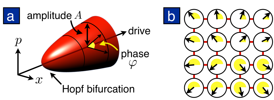
In the system that we study, all oscillators are undergoing motion on a limit cycle, see Fig. 1. We start with the following equations (“Hopf equations”), which describe the effective phase and amplitude dynamics of these resonators close to the limit cycle [8, 13]:
| (1) |
Here is the frequency at the steady-state amplitude . The frequency-pull due to amplitude changes has been kept to leading order in the first line, is the rate at which the amplitude is forced back to the limit cycle, and is the total force exerted on resonator . For the physically most relevant spring-like coupling between nearest neighbors, which will be studied here, the force is given as . The coupling constant is , and indicates nearest neighbor sites.
We consider the case of weak coupling and assume , . Then the amplitude fluctuations around the steady state value are small and the amplitude dynamics can be integrated out (for details on this step, also about disorder, see [8, 13] and the Supplemental Material (SM)). We arrive at effective equations for the resonator phases. Keeping only the slow phase dynamics (and assuming identical resonators), we get
| (2) |
with , , . We will call Eq. (2) the Hopf-Kuramoto model. It has been derived before in the context of optomechanics [8, 13], but it holds generally for a set of weakly coupled Hopf oscillators. Our aim is to explore the dynamics of this model on a square lattice.
The term of Eq. (2) is well known from the Kuramoto model [17], or, equivalently, the XY model [20]. Here the term arises from the amplitude-dependence of the frequency [5]. Both contributions in the first line of Eq. (2) have been derived previously for coupled limit-cycle oscillators, see [21]. They are linear in the coupling . In contrast, the prefactor is of second order in . However, as discussed below, in realistic scenarios and can become small, such that the regime is easily reached. The -term can then have a profound influence on the pattern formation dynamics. The additional contribution also displays next-to-nearest-neighbor coupling of the phases, in spite of the underlying intrinsic nearest-neighbor coupling in the lattice assumed here.
We will first set the stage by highlighting several limiting cases of our model, some of which are known already. For , Eq. (2) can be rewritten in the form . Hence, the system will slide down to a minimum of the potential . In contrast, for non-vanishing , such a potential does not exist and the system may never reach a stationary state (where is constant). The limiting case of Eq. (2) with has been studied before [22, 23, 24, 25, 26]. This is the Sakaguchi-Kuramoto model, usually written in the form with and .
The continuum limit of Eq. (2), which is valid for smooth phase fields, is given by
| (3) |
where , with lattice constant . In this model (with ) it has been found that spirals can develop around singularities in the phase field [27, 24]. Besides, it has been analyzed in connection with chemical turbulence in one dimension [28, 29, 30].
The aim of this paper is to explore pattern formation in the full model, Eq. (2), in large two-dimensional arrays. Our main result is the pattern phase diagram discussed further below. The patterns we find will determine the phase synchronization dynamics of limit-cycle oscillators.
Our numerical results are mostly obtained from simulations with a random initial phase field, since that is the natural starting point in real systems (e.g. after switching on the pump laser or the feedback driving the oscillators into the limit cycle). After some transient dynamics, we often find patterns that do not change qualitatively any more on longer time scales. Moreover, in certain parameter regimes, we find nontrivial stationary patterns.
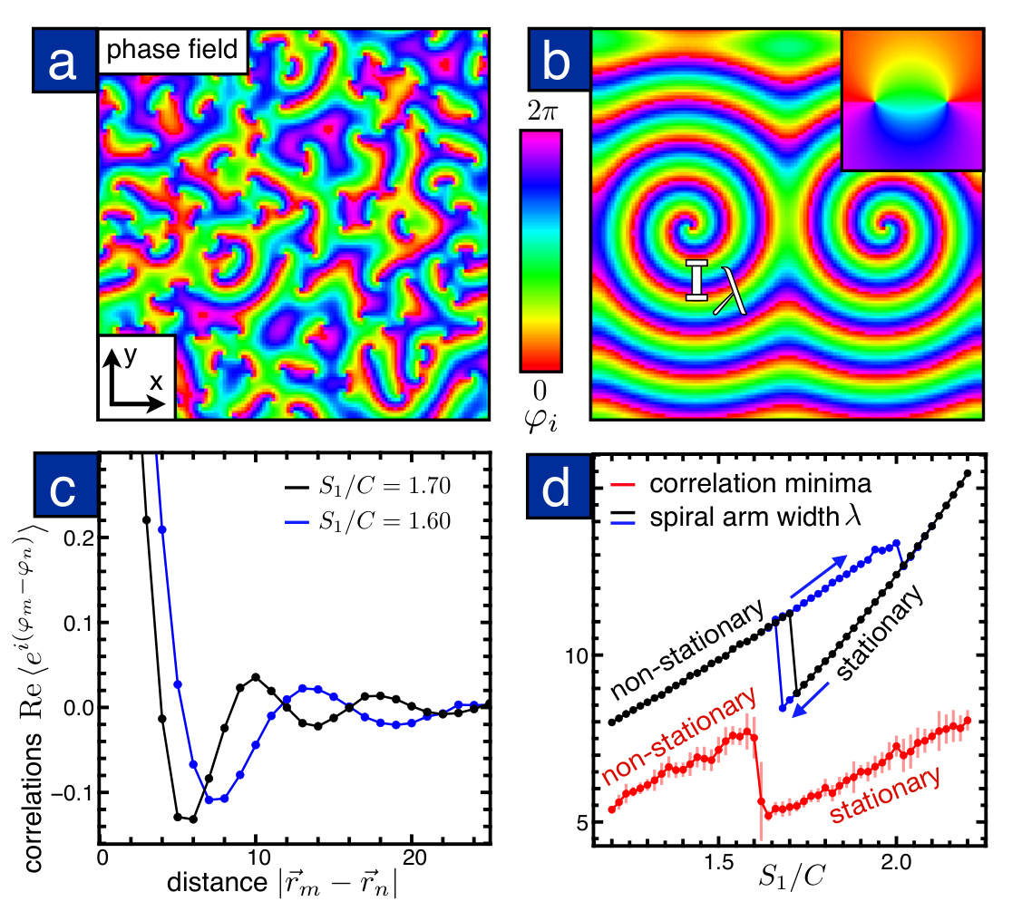
A typical final pattern of a simulation with large is shown in Fig. 2a. This pattern is stationary. It consists of many vortex-like “singularities”, where the phase changes by when going around in a closed loop. These points are surrounded by spiral structures. Spiral patterns in general are well-known as a recurring motif in pattern formation [19, 31]. Since they form an important part of the patterns we observe, we now briefly discuss the properties of isolated spirals, produced from an initial condition with a vortex in the phase field (Fig. 2b).
It is known that in related models, there is a transition from stationary spirals to non-stationary spirals, i.e. a situation when the spiral centers are no longer phase-locked to the bulk of the lattice [23, 32]. We have discovered that this transition also gives rise to a jump in the width of the spiral arms, (Fig. 2). Outside of the jump, increases with increasing and (black curve in Fig. 2d). When sweeping the parameter ratio up and down, we find hysteresis in the spiral arm width (blue line in Fig. 2d). The precise value at which the jump occurs can then depend on the parameter sweep rate. Our analysis illustrates that the microscopic details of the spiral center, on the scale of a few lattice sites, influence both the spiral arm width and the macroscopic pattern considerably. Because the structure of the spiral core is complicated, we cannot provide an analytical prediction for .
We now turn to the statistical properties of the patterns which evolve out of random initial conditions (see Fig. 2a), as they are directly relevant for experiments. The spatial correlations of the phase field are characterized by the correlator , whose distance dependence is displayed in Fig. 2c. We find an oscillatory structure connected to the presence of spiral arms. On top of that, there is an exponential decay, due to the presence of many randomly located spiral centers. The position of the first minimum in the oscillations indicates the distance approximately set by half a spiral arm width. The dependence of this distance on the parameter is shown as the red line in Fig. 2d. Again, we find a sudden jump associated with the transition from stationary to non-stationary spiral centers. We note that the spiral arm width determined for isolated spirals does not agree completely with the length scale extracted from the oscillations of the correlator. The difference can be traced back to changes in the spiral core produced by the presence of other nearby spirals.
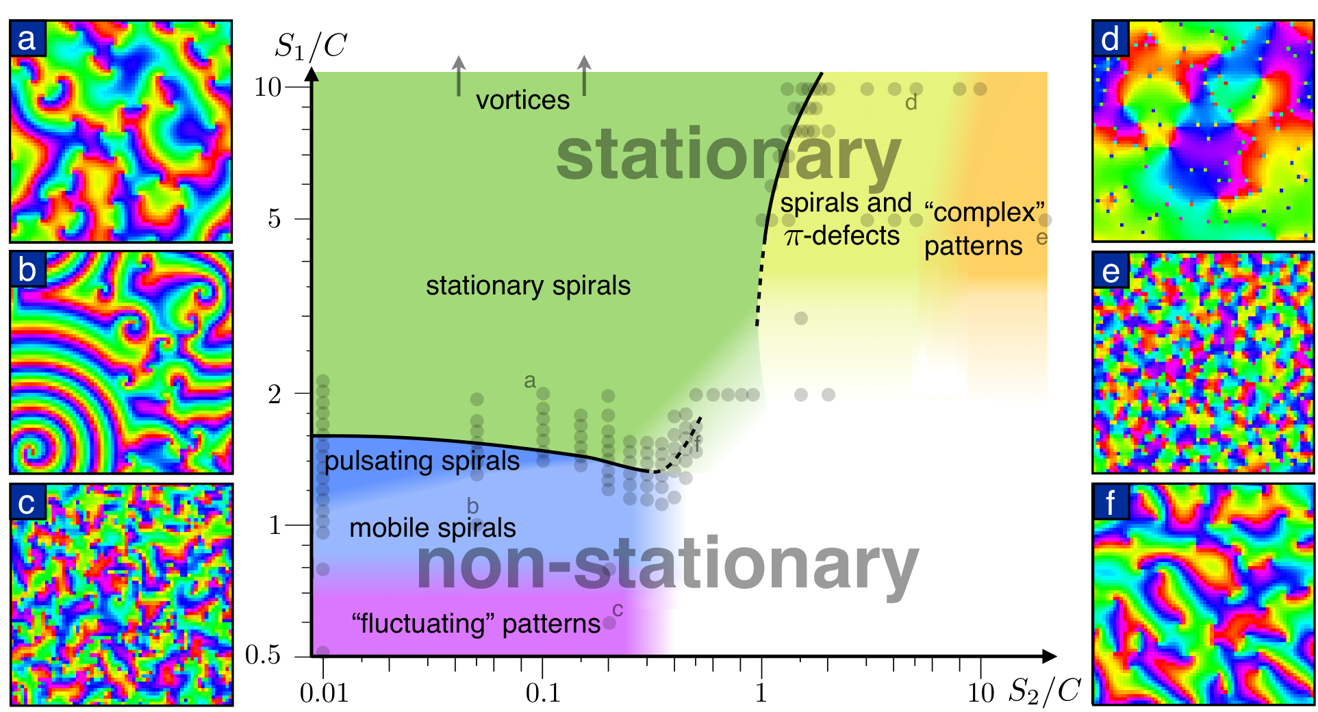
There are only two dimensionless parameters, and , that determine the properties of the final pattern. Therefore, a complete overview of the various regimes in our model is provided by the “pattern phase diagram” in Fig. 3. This summarizes the main results of our studies, and we now explain its features.
The transition discussed above, between stationary and non-stationary spirals, is sharp and can be traced up to intermediate values of . In addition, we find two classes of non-stationary spirals: “pulsating” spirals, where the core keeps orbiting in a small circle around a fixed location [32], and truly mobile spirals that move through the whole lattice. We will comment on their dynamics later. We have not observed a sharp transition between the two regimes (Fig. 3). At larger , the transition is directly from stationary to mobile spirals.
When decreasing the parameter even further, we find a crossover to “fluctuating” patterns, see Fig. 3c. These are non-stationary patterns with a complicated phase structure on the scale of the lattice. For the special case , the location of the crossover (around ) matches the result obtained in [25].
The crucial macroscopic length scale of the Hopf-Kuramoto model, i.e. the spiral arm width, grows with increasing . In view of that, it is surprising to see microscopic structures appearing at larger values of this parameter. Indeed, we find a sharp transition from the domain of “stationary spirals” to stationary patterns that contain “-defects”, see Fig. 3d. These are point defects which are offset by a phase difference of roughly from the smooth surrounding phase field. The stability of a single -defect on a homogeneous background can be analyzed by semi-analytical linear stability analysis (in the limit ; for details, see the SM), which gives the critical value . This defines the asymptote for the transition line in Fig. 3. Above the critical value, the -defect patterns form a fixed point of the dynamics and can be reached from random initial conditions. In contrast to the pure spiral patterns, these patterns resolve the structure of the lattice and hence form a fundamentally different phase. Obviously, they cannot appear in the continuum model, Eq. (3).
When increasing the parameter value further, the density of -defects increases until we observe a smooth transition to “complex” patterns. These are stationary patterns with a complicated phase structure on the scale of the lattice, see Fig. 3e.
Finally, we note that the white region in the phase diagram could not be accessed due to the significant increase of timescales. Apart from that, we have discussed all phases in the Hopf-Kuramoto model, for positive parameters. Changing the sign of or will not give qualitatively different results: The emerging patterns can be reconstructed from the patterns discussed above by the transformations for a sign change of , and /2 (“checkerboard gauge”) for a sign change of . This works for all values of . However, changing the sign of will lead to different patterns. These involve structure on the scale of the lattice, where phase differences of roughly play an important role. We will not discuss these patterns, because for coupled Hopf oscillators is positive.
We now turn to a more detailed discussion of the spiral motion and interaction (see also [33] for the continuum case, at ). Whenever we observe mobile spirals, a fraction of the spirals and anti-spirals eventually annihilate. In some cases, they can also be created dynamically. We observe that the spirals move through the array almost independent of one another for small , whereas they tend to move in pairs for larger values of this parameter. For large values of , mobile and stationary spirals can even coexist, see Fig. 4. Depending on initial conditions, the final state can then be non-stationary or stationary (if all mobile spirals annihilate).
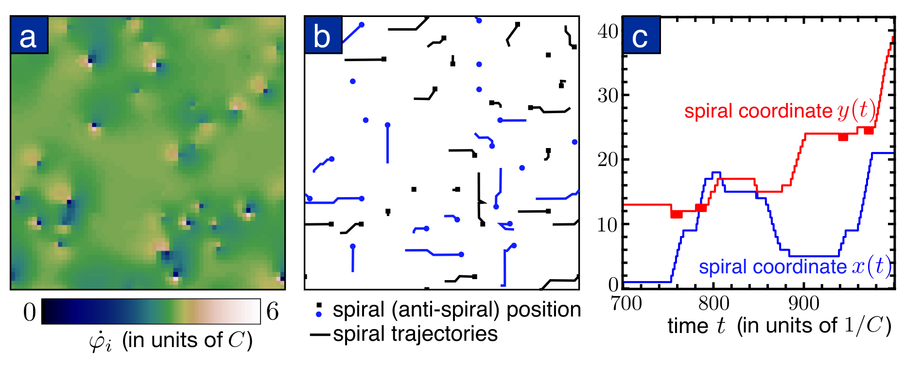
There is also a parameter regime where -defects, stationary and mobile spirals can all be present and interact: Upon the annihilation of a spiral-anti-spiral pair, a -defect can be left behind. This happens more often for larger values of . When a mobile spiral approaches a -defect, it can induce the dissolution of the defect into a spiral-anti-spiral pair. However, the mobile spiral can also move across the defect and make it vanish. All these interactions play an important role even at late times.
Experimental studies of the patterns discussed in this work could be implemented by direct local electrical readout of the motion in electrically coupled nanomechanical resonator arrays [3], or by optical readout of the motion in future optomechanical arrays [8, 13] based on optomechanical crystals [34, 35] or other platforms. The latter consist of an array of localized mechanical modes, each of them coupled to one localized optical mode, driven by a laser. The model parameters could be tuned by varying the laser power and detuning. Simulations of single optomechanical cells, where we extracted the phenomenological parameters , and , suggest that all the important regions of the pattern phase diagram could be explored. Near the Hopf bifurcation, can be reached (since ), so . Furthermore, holds as well for sufficient coupling , when . The motion can be read out by observing the light scattered from the sample. The intensity of the light scattered with wave vector transfer is related to the structure factor (see SM), i.e. the spatial Fourier transform (at ) of the phase correlator . In a typical experiment, the frequencies will be disordered, but first simulations (with standard deviation ) do not show qualitative changes of the patterns we discussed. However, initially mobile spirals could be pinned at sites with lower frequencies [23].
The variety of patterns summarized in Fig. 3 are important for synchronization dynamics and applications. For example, finite phase-differences across the array (in stationary patterns) will reduce the total power output of the collective oscillator, and the mere presence of spirals can reduce the robustness against noise [9]. Finite frequency-differences (in non-stationary patterns) reduce the frequency stability. Tuning the parameters into suitable regions will optimize the array’s properties. Future theoretical studies of the Hopf-Kuramoto model could include noise, which may lead to interesting effects, as discussed for similar models in [18]. In that context, as well as in the deterministic case, the role of spiral motion and interaction could be analyzed in more detail.
Acknowledgements.
We acknowledge support from an ERC Starting Grant, the DARPA program ORCHID, and the ITN cQOM. We thank Ron Lifshitz for helpful discussions.References
- [1] J. Kurths, A. Pikovsky, and M. Rosenblum, Synchronization: A Universal Concept in Nonlinear Sciences (Cambridge University Press, Cambridge, England, 2001).
- [2] M. Bagheri, M. Poot, L. Fan, F. Marquardt, and H. X. Tang, Phys. Rev. Lett. 111, 213902 (2013).
- [3] M. H. Matheny, M. Grau, L. G. Villanueva, R. B. Karabalin, M. C. Cross, and M. L. Roukes, Phys. Rev. Lett. 112, 014101 (2014).
- [4] M. Zhang, G. S. Wiederhecker, S. Manipatruni, A. Barnard, P. McEuen, and M. Lipson, Phys. Rev. Lett. 109, 233906 (2012).
- [5] M. C. Cross, A. Zumdieck, R. Lifshitz, and J. L. Rogers, Phys. Rev. Lett. 93, 224101 (2004).
- [6] M. C. Cross, J. L. Rogers, R. Lifshitz, and A. Zumdieck, Phys. Rev. E 73, 036205 (2006).
- [7] C. Holmes, C. Meaney, and G. Milburn, Phys. Rev. E 85, 066203 (2012).
- [8] G. Heinrich, M. Ludwig, J. Qian, B. Kubala, and F. Marquardt, Phys. Rev. Lett. 107, 043603 (2011).
- [9] J.-M. A. Allen and M. C. Cross, Phys. Rev. E 87, 052902 (2013).
- [10] M. C. Cross, Phys. Rev. E 85, 046214 (2012).
- [11] T. E. Lee and M. C. Cross, Phys. Rev. Lett. 106, 143001 (2011).
- [12] G. Giorgi, F. Galve, G. Manzano, P. Colet, and R. Zambrini, Phys. Rev. A 85, 052101 (2012).
- [13] M. Ludwig and F. Marquardt, Phys. Rev. Lett. 111, 073603 (2013).
- [14] A. Mari, A. Farace, N. Didier, V. Giovannetti, and R. Fazio, Phys. Rev. Lett. 111, 103605 (2013).
- [15] S. Walter, A. Nunnenkamp, and C. Bruder, Annalen der Physik (2014), 10.1002/andp.201400144.
- [16] T. Lee and H. Sadeghpour, Phys. Rev. Lett. 111, 234101 (2013).
- [17] Y. Kuramoto, in International Symposium on Mathematical Problems in Theoretical Physics, Lecture Notes in Physics, Vol. 39, edited by H. Araki (Springer Berlin Heidelberg, 1975) pp. 420–422.
- [18] J. Acebrón, L. Bonilla, C. Pérez Vicente, F. Ritort, and R. Spigler, Rev. Mod. Phys. 77, 137 (2005).
- [19] M. C. Cross and P. C. Hohenberg, Rev. Mod. Phys. 65, 851 (1993).
- [20] J. M. Kosterlitz and D. J. Thouless, Journal of Physics C: Solid State Physics 6, 1181 (1973).
- [21] R. Lifshitz, E. Kenig, and M. C. Cross, in Fluctuating Nonlinear Oscillators, edited by M. I. Dykman (Oxford University Press, Oxford, 2012) Chap. 11.
- [22] H. Sakaguchi and Y. Kuramoto, Progress of Theoretical Physics 76, 576 (1986).
- [23] H. Sakaguchi, S. Shinomoto, and Y. Kuramoto, Progress of Theoretical Physics 79, 1069 (1988).
- [24] Y. Kuramoto, Progress of Theoretical Physics Supplement 79, 223 (1984).
- [25] P.-J. Kim, T.-W. Ko, H. Jeong, and H.-T. Moon, Phys. Rev. E 70, 065201 (2004).
- [26] K. Wiesenfeld, P. Colet, and S. H. Strogatz, Phys. Rev. E 57, 1563 (1998).
- [27] Y. Kuramoto and T. Yamada, Progress of Theoretical Physics 56, 724 (1976).
- [28] T. Yamada and Y. Kuramoto, Progress of Theoretical Physics 56, 681 (1976).
- [29] Y. Kuramoto and T. Tsuzuki, Progress of Theoretical Physics 55, 356 (1976).
- [30] Y. Kuramoto, Progress of Theoretical Physics 63, 1885 (1980).
- [31] A. T. Winfree, Science 175, 634 (1972).
- [32] J. E. Paullet and G. B. Ermentrout, SIAM Journal on Applied Mathematics 54, 1720 (1994).
- [33] I. S. Aranson, L. Kramer, and A. Weber, Phys. Rev. Lett. 67, 404 (1991).
- [34] M. Eichenfield, J. Chan, R. M. Camacho, K. J. Vahala, and O. Painter, Nature 462, 78 (2009).
- [35] A. H. Safavi-Naeini, J. T. Hill, S. Meenehan, J. Chan, S. Gröblacher, and O. Painter, Phys. Rev. Lett. 112, 153603 (2014).
Supplemental Material for “Pattern phase diagram for 2D
arrays of coupled limit-cycle oscillators”
Roland Lauter,1,2,∗ Christian Brendel,1 Steven J. M. Habraken,1 and Florian Marquardt1,2
1Institut für Theoretische Physik II, Friedrich-Alexander-Universität
Erlangen-Nürnberg, Staudtstr. 7, 91058 Erlangen, Germany
2Max Planck Institute for the Science of Light, Günther-Scharowsky-Straße 1/Bau 24, 91058 Erlangen, Germany
I Derivation of the Hopf-Kuramoto model
In this section, we derive the Hopf-Kuramoto model from the following general Hopf equations
| (S.1) | ||||
| (S.2) |
Here, is the amplitude-dependent frequency of the oscillator at site , is its mass, is its steady-state amplitude and is the frequency at the steady-state amplitude. Other symbols have the same meaning as in the main text. The second term on the right-hand side of Eq. (S.1) arises from the expansion of around the steady-state amplitude . For reasons that will become clear later, has not been expanded in the force terms in Eqs. (S.1) and (S.2). We assume that the oscillators are coupled by spring-like nearest-neighbor couplings so that the forces are given by
| (S.3) |
where denotes the nearest neighbors of site and are spring constants.
The derivation of the Hopf-Kuramoto model involves the adiabatic elimination of the amplitude fluctuations , as well as leading-order expansions in the dimensionless, small parameters , and . These parameters and the relative amplitude fluctuations are assumed to be of the same order of smallness. Below, we will also only keep slowly varying terms. The derivation can also be found in [1]. For some more details, see the Supplemental Material of [2].
In order to eliminate the amplitude fluctuations, we rewrite Eq. (S.2) in terms of the amplitude fluctuations and formally integrate the equation
| (S.4) |
to obtain the long-time limit result
| (S.5) |
Since the integrand is proportional to , to leading order it suffices to evaluate to zeroth order in the expansion parameters, i.e. . Thus, we find
| (S.6) |
The integral can easily be evaluated. To leading order in , the result reduces to
| (S.7) |
To first order in the amplitude fluctuations, the equations of motion for the oscillator phases (S.1) can be expanded as
| (S.8) |
Corrections to are proportional to both and so that they are of second order. In the second term on the right-hand side, these are significant, but, since in the third term they are multiplied by another , they can be neglected there. Inserting (S.7), again replacing in the denominator by , we finally obtain
| (S.9) | ||||
where we have also only kept slowly varying contributions by applying the approximations , and . In the special case of identical oscillators , and for all and uniform couplings for all neighbors , this obviously reduces to equation (2) in the main text, where we have also neglected the trivial term on the right hand side.
II Semi-analytical stability analysis of point defects
In this section, we present the analysis of the stability of a single -defect on a homogeneous background phase field for the Hopf-Kuramoto model (Eq. (2) in the main text) with . For this case, the aforementioned phase configuration, which we call , is a fixed point of the dynamics, i.e. for all sites . Besides, the equation of motion can be written as with the potential
We calculate the Hessian and evaluate its eigenvalues for the phase configuration numerically. If at least one of the eigenvalues is negative, the configuration is unstable. A single eigenvalue, corresponding to the translational mode of the system, might vanish without disturbing our analysis. We always find this zero eigenvalue. For small values of , all the other eigenvalues are positive, which means that -defects are stable (see Fig. S.1). With increasing , the eigenvalues change linearly with this parameter. A single eigenvalue has a negative slope, so it becomes negative at some critical value , rendering the phase configuration unstable. This gives the (inverse) value given in the main text.

III Read-out of the mechanical resonator phase field
Here, we will show how the intensity of the light reflected from an optomechanical array is related to the spatial Fourier transform of the phase correlator. The intensity of the light reflected from an optomechanical array with lattice sites at is given as
| (S.10) |
The phase of the light reflected from site is , where depends on the system parameters. If the mechanical frequency is much smaller than the cavity intensity decay rate , then , with the mechanical amplitude and the optical frequency shift per displacement [3]. For small , Eq. (S.10) can be expanded and we get
| (S.11) |
We average over time, use and , and arrive at
| (S.12) |
For large arrays, the first term will only give contributions very close to . For small arrays, these contributions may have to be eliminated by calibrating the measurement device with a known phase field. The second term can be evaluated to give
| (S.13) |
On the right-hand side of this equation, the discrete Fourier transform of the correlations in the system appears. We have analyzed similar correlation functions in connection with the spiral length scale, see Fig. 2 in the main text. From Eq. (S.13) we see that we can learn about the correlations by detecting the intensity of the reflected light. An example for the part of the detected light intensity that is given in Eq. (S.13) is given in Fig. S.2.
References
- [1] G. Heinrich, M. Ludwig, J. Qian, B. Kubala, and F. Marquardt, Phys. Rev. Lett. 107, 043603 (2011).
- [2] M. Ludwig and F. Marquardt, Phys. Rev. Lett. 111, 073603 (2013).
- [3] M. Aspelmeyer, T. J. Kippenberg, and F. Marquardt, Rev. Mod. Phys. (2014), in press; arXiv: 1303.0733 (2013) .