Co-evolution of Extreme Star Formation and Quasar: hints from Herschel and the Sloan Digital Sky Survey
Abstract
Using the public data from the Herschel wide field surveys, we study the far-infrared properties of optical-selected quasars from the Sloan Digital Sky Survey. Within the common area of , we have identified the far-infrared counterparts for quasars, among which are highly secure detections in the Herschel band (signal-to-noise ratios ). This sample is the largest far-infrared quasar sample of its kind, and spans a wide redshift range of . Their far-infrared spectral energy distributions, which are due to the cold dust components within the host galaxies, are consistent with being heated by active star formation. In most cases (%), their total infrared luminosities as inferred from only their far-infrared emissions () already exceed , and thus these objects qualify as ultra-luminous infrared galaxies. There is no correlation between and the absolute magnitudes, the black hole masses or the X-ray luminosities of the quasars, which further support that their far-infrared emissions are not due to their active galactic nuclei. A large fraction of these objects () have star formation rates . Such extreme starbursts among optical quasars, however, is only a few per cent. This fraction varies with redshift, and peaks at around . Among the entire sample, objects have secure estimates of their cold-dust temperatures (), and we find that there is a dramatic increasing trend of with increasing . We interpret this trend as the envelope of the general distribution of infrared galaxies on the (, ) plane.
Subject headings
infrared: galaxies; galaxies: starburst; galaxies: high-redshift, galaxies: evolution, (galaxies:) quasars: generalI. Introduction
Ultra-Luminous InfraRed Galaxies (ULIRGs), discovered as a distinct class in the early 1980’s [29, 28, 1] by the Infrared Astronomical Satellite (IRAS) survey of the sky in 12 to , are believed to host extreme star formation regions that are heavily enshrouded by dust. They are characterized by their exceptionally high IR luminosities (; integrated over restframe 8 to ), which are believed to be predominantly due to the re-radiation of star light processed by dust (see Lonsdale et al. 39 for a review), and thus imply very high star formation rates (SFR) of (using the conversion of Kennicutt 33) completely hidden by dust.
However, it has been noticed ever since their discovery that a significant fraction of ULIRGs, especially those very luminous ones, have optical signatures indicative of classic AGN activities. For examples, Carter [8] notes that ten among a sample of 13 IRAS sources with flux density are Seyfert galaxies. Sanders et al. [66] show that ten galaxies among the 324 sources with from the IRAS Bright Galaxy Survey are ULIRGs and that they all have a mixture of starburst and AGN signatures, which has led them to propose an evolutionary scenario that ULIRGs are the prelude to quasars. In their redshift survey of the IRAS galaxy sample, Lawrence et al. [35] have found that of their 95 ULIRGs are AGN. The consensus is that ULIRGs that have “warm” IR colors, i.e., whose emissions tend to peak at restframe mid-IR (MIR) rather than far-IR (FIR), generally host (optical) AGN, which could be the main energy sources that power their strong IR emissions [15, 49, 34, e.g.,]. On the other hand, “cold” ULIRGs that have their IR emissions peak at FIR should be mostly powered by starbursts [19, 26, e.g.,].
An interesting question then is whether any AGN ULIRGs, especially quasar ULIRGs, have starbursts that dominate their IR emissions. Quasars represent the most extreme process of supermassive black hole accretion, while starbursts are the most extreme process of star formation. It is expected that the interplay of these two extremes will have important consequences. This is made particularly important by the quasar evolutionary scenario of Sanders et al. [66], as such objects could be the transitional type between non-quasar ULIRGs and “fully exposed” quasars. Sanders et al. themselves believe that AGN heating is the main mechanism for the strong IR emission of ULIRG quasars. In their discussion of PG quasar continuum distributions from UV to millimeter (mm), Sanders et al. [65] further propose that a warped galactic disk (beyond the central to a few ) heated by the central AGN can explain the entire range of IR emission from to . However, Rowan-Robinson [63] argues that this scheme could only be viable when the total luminosity in IR is comparable or less than that in UV-optical; instead, he has successfully modeled the IRAS-detected PG quasars by attributing their mid-IR emissions to AGN heating and the FIR emission to starburst heating, respectively. More analysis using larger samples from the Infrared Space Observatory (ISO) observations support this view. For example, Haas et al. [24] have studied 64 PG quasars and have concluded that starburst heating is more likely the cause of the observed cold dust () FIR emissions among the ULIRG part of the sample. However, they have also pointed out that AGN heating should be the main power source for those extreme ones that qualify as “Hyper-luminous Infrared Galaxies” (HyLIRG; usually defined by ).
There are also two pieces of important, albeit indirect, evidence supporting that the FIR emissions of quasar ULIRGs are likely due to starbursts. First, a significant fraction of such objects have a large amount of molecular gas [66, 20, 69, 86, e.g.,], which is a strong indicator of active star formation. Second, most quasar ULIRGs have polycyclic aromatic hydrocarbon (PAH) features, which are also strongly indicative of on-going star formation [68, 74, 25, 46, 7, e.g.,]. While none of these are sufficient to assert that starbursts dominate the strong FIR continua of quasar ULIRGs, it is clear that they at least contribute significantly.
The picture above is largely based on the ULIRGs in the nearby universe where they can be studied in detail. It would not be surprising if any of it changes at high redshifts, as both quasars and ULIRGs evolve strongly. The number density of quasars rises rapidly from to , and reaches the peak at [48, e.g.,]. Similarly, while ULIRGs are very rare objects today, they are much more numerous in earlier epochs. The deep ISO surveys have revealed a large number of IR-luminous galaxies, among which are ULIRGs and many are at [64, e.g.,]. The discovery of the so-called “submillimeter (submm) galaxies” (SMGs) at 450 and (see Blain et al. 5 for a review) added a new population to the ULIRG family, as most of them are at and have dominated by the emission from cold dust. Furthermore, Spitzer observations suggest that high stellar mass () and otherwise “normal” star-forming galaxies at are likely all ULIRGs [11, e.g.,], which increases the ULIRG number density at high redshifts to a more dramatic level than expected. On the other hand, molecular gas has also been detected in quasar ULIRGs from to 6 (Solomon & Vanden Bout 77, and the references therein; see also e.g., Wang et al. 83, Wang et al. 84, Wang et al. 85 for the recent results at ), lending support to the starburst-powered interpretation of the FIR emission of such objects at high redshifts as well.
If quasars and dust-enshrouded starbursts do co-exist, it is important to investigate their co-evolution, which would require a large sample over a wide redshift range. Herschel Space Observatory [52] has offered an unprecedented opportunity to investigate this problem at the FIR wavelengths that were largely unexplored by the previous studies. Herschel had two imaging instruments, namely, the Photodetector Array Camera and Spectrometer [53, PACS,] and the Spectral and Photometric Imaging REceiver [23, SPIRE,]. The PACS bands are 100 (or 70) and , and the SPIRE bands are 250, 350 and . Together they sample the peak of heated dust emission from to 6 and beyond. There already have been a number of studies on the FIR emission of quasars using Herschel observations [70, 36, 37, 12, 45, e.g.,], however the current collection of quasars that have individual Herschel detections are still very scarce in number and few have spanned a sufficient redshift range (for examples, Leipski et al. [37] present 11 objects at ; Dai et al. [12] include 32 objects at ; Netzer et al. [45] report ten within a narrow window at ).
In this paper, we present a large sample of optical quasars that are detected by the Herschel, and provide our initial analysis of their FIR properties. The quasars are from the Sloan Digital Sky Survey [88, SDSS;], and the FIR data are from the public releases of four major wide field surveys by Herschel, namely, the Herschel Astrophysical Terahertz Large Area Survey [18, H-ATLAS;], the Herschel Multi-tiered Extragalactic Survey [47, HerMES;], the Herschel Stripe 82 Survey [81, HerS;], and the PACS Evolutionary Probe [40, PEP;]. We describe the data and the sample construction in §II, and present our analysis of the FIR dust emission in §III. The implications of our results are detailed in §IV, and we conclude with a summary in §V. The catalog of our sample is available as online data in its entirety. All quoted magnitudes in the paper are in the AB system. We adopt the following cosmological parameters throughout: , and .
II. Data description and sample construction
In brief, we built our sample by searching for the counterparts of the SDSS quasars in the Herschel wide field survey data. For the sake of simplicity, hereafter we refer to these objects as “IR quasars”. We describe below the data used in our study and the constructed IR quasar sample.
II.1. Parent quasar samples


The parent quasar samples that we used are based on the SDSS Data Release 7 and 10 quasar catalogs (hereafter DR7Q and DR10Q, respectively), which are summarized as follows.
- DR7Q
-
As detailed in Schneider et al. [67], this quasar catalog is based on the SDSS DR7. It concludes the quasar survey in the SDSS-I and SDSS-II over , and supersedes all previously released SDSS quasar catalogs. It includes quasars between and 5.46 (the median at ), all with absolute -band magnitudes () brighter than .
- DR10Q
-
This quasar catalog is derived from the on-going Baryon Oscillation Spectroscopic Survey (BOSS) as part of the SDSS-III. While it was released in the SDSS DR10, its main target selection was based on the SDSS DR8. The detailed description of the catalog can be found in Pâris et al. [50]. It includes new quasars with from the SDSS-III, where is the absolute magnitude -corrected to [50, for details, see]. It also includes a large number of known quasars of similar characteristics (mostly from SDSS-I and II) that were re-observed by BOSS. In brief, the catalog contains quasars over , with redshifts ranging from 0.05 to 5.86.
The quasars from these two catalogs are largely independent, however there are still of them being duplicates, which we define as the ones falling within a matching radius of . Figure 1 shows the comparison of the photometry, the redshift measurements and the absolute magnitudes from these two catalogs for this overlapped population, which all agree reasonably well. For the sake of simplicity, we adopt the DR10Q values in this work for these duplicates unless noted otherwise.
In the end, we produced a merged sample of unique quasars, which represents the largest optical quasar sample selected based on the most homogeneous data set over the widest area to date. The redshift distributions of DR7Q, DR10Q and the merged catalog are shown in Figure 2. For simplicity, hereafter we refer to the merged sample as the “SDSS quasar sample” and the quasars therein as the “SDSS quasars”. We note that DR7Q and DR10Q are statistically different samples, and therefore any statistical results from this merged catalog should be inferred with caution. This is exacerbated by the fact that the quasars were not selected uniformly within either DR7Q or DR10Q, as detailed in Schneider et al. [67] and Pâris et al. [50], respectively. For example, while most of the quasars in DR7Q were selected using the algorithms as described in Richards et al. [55] (with USELFLAG=1 in the catalog), a non-negligible fraction of them were selected early in the SDSS campaign when such algorithms had not yet been fully developed. DR10Q is even more non-uniform in this sense, because only about half of its quasars (called the “CORE” sample) were selected uniformly (with UNIFORM>0 in the catalog) through the XDQSO method [6] and the other half (called the “BONUS” sample) were selected using various different methods [61, see]. Nevertheless, the non-uniformity does not affect our current work since we limit our study to the FIR properties of optical-selected quasars, whose being selected did not use any FIR information and thus should not favor or against any given FIR property.
II.2. Herschel Data
| Survey | Field | Level | Coverage | limit | All aafootnotemark: | Match | SNR | |
|---|---|---|---|---|---|---|---|---|
| () | () | |||||||
| HerMES | COSMOS bbfootnotemark: | L1 | 5.00 | 31.4 | 216 | 47 | 7 | 3 |
| GOODS-North bbfootnotemark: | L2 | 0.63 | 27.1 | 17 | 4 | 1 | 1 | |
| Bootes-HerMES | L5 | 11.29 | 31.3 | 426 | 50 | 18 | 2 | |
| EGS-HerMES bbfootnotemark: | L5 | 3.12 | 29.7 | 53 | 6 | 3 | 0 | |
| (Groth-Strip) | L3 | 30.9 | 3 | 2 | 0 | |||
| ELAIS-N1-HerMES | L5 | 3.74 | 30.4 | 22 | 3 | 3 | 0 | |
| Lockman-SWIRE bbfootnotemark: | L5 | 19.73 | 37.0 | 276 | 35 | 12 | 5 | |
| (Lockman-East-ROSAT) | L3 | 31.5 | 1 | 0 | 0 | |||
| (Lockman-North) | L3 | 31.4 | 2 | 1 | 0 | |||
| FLS | L6 | 7.30 | 35.4 | 89 | 17 | 5 | 3 | |
| XMM-LSS-SWIRE | L6 | 21.61 | 48.5 | 402 | 25 | 3 | 3 | |
| (UDS) | L4 | 33.8 | 3 | 1 | 0 | |||
| (VVDS) | L4 | 33.7 | 8 | 2 | 0 | |||
| HerS | Stripe82 | L7 | 80.76 | 51.8 | 4519 | 132 | 58 | 53 |
| HATLAS | SDP | N/A | 19.28 | 34.1 | 690 | 18 | 18 | 12 |
| Total | 172.46 | 6710 | 354 | 134 | 82 |
We utilized all high-level, publicly available data from the wide field Herschel surveys. In all cases we adopted the latest catalogs released by the survey teams to construct the FIR spectral energy distributions (SEDs). The basic characteristics of these surveys are summarized in Table 1, and their relevant details are briefly described below.
II.2.1 HerMES
HerMES was the largest Herschel guaranteed time key program, and surveyed in six levels of depth and spatial coverage combinations (“L1” to “L6”), using both SPIRE and PACS. Its latest data release, “DR2”, contains the SPIRE maps and the source catalogs in all three bands [82]. The PACS data have not yet been released. In this work, we used the wide-field data and excluded those galaxy cluster fields.
The HerMES DR2 includes two sets of source catalogs based on different methods, one using the SUSSEXtractor (SXT) point source extractor and the other using the iterative source detection tool StarFinder (SF) combined with the De-blended SPIRE photometry algorithm (DESPHOT). We adopted the band-merged version of the latter (denoted as “xID250”in DR2), which has the DESPHOT multi-band (250, 350 and ) photometry at the positions of the SF sources. The detection limits in range from to in our fields of interest.
II.2.2 H-ATLAS
H-ATLAS was the largest Herschel open-time key program. It surveyed using both SPIRE and PACS. Currently, this program has released the image maps and the source catalogs in the field observed during the Herschel Science Demonstration Phase [30, 51, 58, H-ATLAS SDP;], which covers and has reached the limit of in .
The catalog that we adopted is the band-merged one with both the SPIRE and the PACS photometry. For the SPIRE bands, the source extraction was done using the Multi-band Algorithm for source eXtraction , which employed a localized background removal and PSF filtering procedures to the map and extracted the sources using the positions as the priors. For the PACS bands, aperture photometry was performed on the 100 and maps at the SPIRE positions.
II.2.3 HerS
II.2.4 PEP
PEP was also a Herschel guaranteed time key program, which used PACS to survey six well-studied extragalactic fields and also a number of galaxy clusters. Both the image maps and the source catalogs have been made public through Data Release 1 (DR1) of the team. These data are not listed in Table 1. All the PEP fields are within the HerMES fields, however they only covered a small fraction.
Whenever possible, we used their 100 and measurements in the COSMOS, GOODS-North, EGS, Lockman Hole fields to supplement the HerMES SPIRE photometry to better constraint the FIR SEDs of the detected quasars. These measurements were taken from the SF “blind extraction” catalogs as described in Magnelli et al. [41].
II.3. Herschel-detected quasars
Our IR quasar sample was derived by matching the positions of the SDSS quasars to those of the Herschel sources in the band-merged, -based catalogs as described above.
II.3.1 Matching radius

The matching was performed using
TOPCAT/STILTS11
1
TOPCAT
http://www.starlink.ac.uk/topcat;
STILTS
http://www.starlink.ac.uk/stilts .
We used a matching radius of , which is justified
below.
While the Herschel instruments have large beam sizes 22 2 The FWHM beam sizes are , and for the SPIRE 250, 350 and , respectively, and 6– and 11– for the PACS 100 and , respectively., the source centroids can still be determined to high accuracy. The positional uncertainty of a given source depends on its signal-to-noise ratio (SNR) [31, see, e.g.,], which follows
| (1) |
where and are the nominal uncertainties of RA and Dec, respectively, and is the beam size. The SPIRE beam size is , which means that the positional uncertainty of a given source is
| (2) |
A matching radius of thus corresponds to uncertainty for objects with , or for those with 33 3 We note that Smith et al. [76] use a somewhat different relation between the astrometric uncertainty and the SNR, , which means that uncertainty would be for in . Our results shown in Figure 3 indicate that such a matching radius would be slightly too stringent, and therefore we adhered to our choice.. To further validate our choice, we performed a test using an enlarged matching radius of , and Figure 3 demonstrates the results. The separations between the and the SDSS positions versus the SNR are indeed consistent with the expectation from Equation (2), and the vast majority of the matches within fall within the curve. Furthermore, the separation shows a double-peak feature roughly divided at , indicating that the matches beyond this point are likely affected by other factors, such as the source blending problem (see below).
Wang et al. [82] have addressed the source positional accuracy in the HerMES DR2 catalogs through end-to-end simulations. For the SF catalogs in , they find that the real matches between the input and the output have the positional offsets peak at around . We note that this is derived using the real matches at all SNR levels. If a threshold is applied, this peak is likely to shift to a smaller value. In any case, the matching radius of that we adopted is a rather conservative choice.
In a number of fields the PACS data are also available. The H-ATLAS band-merged catalog in the SDP field already includes the PACS photometry (see §II.2.2) and thus no further action was taken. The HerMES COSMOS, GOODS-N, EGS, and Lockman Hole fields have PACS data from the PEP program (see §II.2.4), and we matched the coordinates in the PEP 100 and “blind” catalogs to both the SPIRE “xID250” catalogs and the SDSS quasars, again using a matching radius of .
II.3.2 Source blending
Due to the large beam sizes of the instruments, Herschel images still suffer from a severe source blending problem. To evaluate how this problem could impact our sample, we visually inspected the Herschel and the SDSS images of all the matches in the test case shown in Figure 3, i.e., using a larger matching radius of . We searched for the signatures of possible source blending, such as the presence of close companions in the SDSS images, and the offset of the source centers among the Herschel bands, etc. For this test, we only used the sources that have in . The result is also shown in Figure 3. As it turns out, enlarging the matching radius from to will include 47 more objects, however only 16 of these 47 objects (34%) are “clean” cases. For comparison, 83% of the sources within the matching radius of are “clean”. This lends further support to our choice of the matching radius. The drawback of using this conservative value is that it could exclude some objects that have genuine Herschel detections but are blended with close neighbor(s). While it is possible to include such sources after using the methods described in Yan et al. [87] to de-blend, we defer this improvement to our future work.
In summary, our conservative choice of the matching radius has resulted in a sample that is free of significant blending problem. This has also simplified the photometry in the SPIRE 350 and bands. While the source catalogs that we adopted from the survey teams were all derived using PSF-fitting based on the detections, the photometry in 350 and would still be prone to large errors introduced by blending due to their much larger beam sizes ( and , respectively). Our relatively clean sample allows us to assume that the fluxes measured in these two redder bands are solely contributed by the source detected in .
II.3.3 IR quasar sample summary
Our Herschel-detected SDSS quasar sample, derived using a matching radius of as described above (Table 1), contains 44 4 We note that there are 18 more matched objects from HerMES DR2 catalogs discarded due to objects in total. Most of our studies are based on a subsample of those, called the “SNR5” sample, which only includes quasars that have in and thus is the sample of the most robust Herschel detections. Based on this SNR5 sample, we further imposed a cut in the flux density, , and formed a “bright” subsample of objects for various discussions below. This flux density threshold was adopted based on the lowest flux density of the SNR5 objects in the shallowest HerMES field L6-XMM-LSS-SWIRE.
III. Dust emission modeling
We inferred the dust emission properties of the IR quasars by fitting their FIR SEDs. The thermal emission over the full IR regime can be viewed as the collective result of all heated dust components of various temperatures, and the FIR part is dominated by the coldest component. In this paper, we focus on this FIR part in the IR quasars and hence our conclusions are pertaining to their cold-dust components. We used two distinct types of models to fit the FIR SEDs, one being a single-temperature, modified blackbody (MBB) spectrum and the other being three different sets of starburst templates. Fitting an MBB spectrum to the FIR SED is always valid, regardless of the exact dust heating sources (i.e., due to photons from either star formation or AGN activity). However, it has the drawback that the SED must be properly sampled in order to obtain well constrained results. Fitting starburst templates, on the other hand, is only appropriate if the FIR emission is dominated by heating from star formation, and the motivation of using these models was to test if the FIR emissions are consistent with being caused by star formation. These two types of SED fitting approach provide independent check to each other, and we will show later that they also lead to insights into the heating sources.
III.1. SED fitting using MBB model


We used the cmcirsed code55 5 http://herschel.uci.edu/cmcasey/sedfitting.html of Casey [9] to perform the MBB fitting, which allowed us to derive the IR luminosity, the dust temperature, and the dust mass. This procedure was only carried out for the objects that have photometry in all the three SPIRE bands ( objects in total, among which are in the SNR5 subsample), because the MBB fit would become unconstrained with less bands.
The FIR emission due to MBB can be written as
| (3) |
where is the characteristic temperature of the MBB, is the scaling factor that is related to the intrinsic luminosity, is the emissivity, and is the reference wavelength where the opacity is unity. As most of our quasars only have three SPIRE bands available, we had to limit the degrees of freedom. We adopted the default emissivity of , which is the value typically assumed for cold dust [9]. By default, cmcirsed sets . We adopted , following Draine [16]. While the exact choice of only marginally affects the estimates of the total IR luminosity and the dust mass, it will significantly impact the estimate of the dust temperature. We will further discuss this effect in Appendix A.
We note that the above form is for general opacity. In the optical thin case, at , the term reduces to , which is often adopted in the submm/mm regime. Throughout this work, we used the general opacity form as in Equation (3).
The cmcirsed code has the capability of superposing a power-law component (PL) to the MBB spectrum to accommodate the possible warm dust component whose effect could be present in the mid-IR regime (typically at in restframe). Thirteen quasars (seven of them are in the SNR5 sample) have PACS data in addition to the three band SPIRE data, and we utilized this capability when fitting these objects. In this case, the MBB+PL model then reads
| (4) |
where is the PL slope, is the normalization of the PL part, and is the turnover wavelength [9, for detail, see ]. Again, to limit the degrees of freedom, had to be fixed, and we adopted the default value of [9].
Recalling that the FIR emission is dominated by the cold-dust component, we can obtain the total IR luminosity of this component as
| (5) |
by integrating the best-fit model from 8 to . For the 13 objects that have PACS data, we also calculated their total IR luminosities as
| (6) |
We emphasize that (here represented by the MBB fit) is the luminosity of the cold-dust component over the entire IR range (). While the bulk of its emission is in the FIR regime, this cold-dust component emits beyond FIR and thus it is necessary to integrate over to capture its total IR luminosity. Note that this is not the total IR luminosity () of the galaxy that includes the contributions of all dust components over . In other words, we have .
The best-fit temperature from cmcirsed was taken as the temperature of the cold dust, i.e., . We also calculated the “peak” temperature inferred from Wien’s displacement law, which is given by
| (7) |
where the coefficient . As compared to , is less sensitive to the specifics of the dust emission models in use and therefore could be a better proxy to the dust temperature when comparing results derived based on different types of templates. For this reason, while we mostly use in this paper, we also use in some occasions. The relation between and is shown in Figure 4. In case of , the relation can be roughly described by the following broken linear function:
| (8) |
III.2. SED fitting using starburst templates
We also fitted the FIR SEDs using three different libraries of starburst galaxies separately, namely, the theoretical model of Siebenmorgen & Krügel [75, hereafter SK07; 7220 templates], and the empirical templates of Chary & Elbaz [10, hereafter CE01; 105 templates] and Dale & Helou [13, hereafter DH02; 64 templates]. For a given quasar, the restframe templates were redshifted according to the quasar’s redshift and convolved with the Herschel passband response curves, and then were compared to the observed IR quasars SEDs. The best-fit template was chosen by minimizing the -square:
| (9) |
We note again that the starburst model fitting was also done for the objects that have photometry in only two or even one SPIRE band. During the fitting, we did not re-scale the templates. By construction, these templates all have associated values (over 8-), and the value of the best-fit template was adopted as the total IR luminosity of the object in question. For clarity, we will refer to it as , where “SB” can be replaced by “SK07”, “CE01” or “DH02” when appropriate. The error of was estimated by taking the difference between the value of the best-fit template and that of the one of the second smallest . As compared to the formal likelihood method, this simple approach has the advantage that it works consistently when the parameter space is discrete, and that it includes the possible systematic errors intrinsic to the template set.
We should emphasize that thus derived is the total IR luminosity of the galaxy. If using the starburst models is appropriate, we should have , where . While cannot be separated from in any of these starburst models, we will show that can help interpret the origin of .
III.3. Dust mass and gas mass
The MBB fit by cmcirsed also resulted in estimate of dust mass (hereafter ). As this quantity is a strong dependent of dust temperature (; see Casey 9), it should be used with caution. For example, in our analysis in §IV, we will only use those that have .
Applying a nominal gas-to-dust ratio, the gas mass () can also be obtained. We adopted the nominal Milky Way gas-to-dust-mass ratio of 140 [17, e.g.] for this work.
IV. Results and discussions
The major physical properties obtained in §III are all given in the online table accompanying this paper. A summary of the information contained in this table is given in Appendix B (see Table 2). Some examples of the SED fitting are also provided in Appendix B. Here we discuss in detail these results, some potential selection effects, and their implications.
IV.1. IR luminosity

For clarity, the various flavors of IR luminosities discussed in §III are summarized here:
- •
: the general designation of the total IR luminosity over ;
- •
: the contribution of the cold-dust component to the total IR luminosity over , which is also referred to as the total IR luminosity of the cold-dust component;
- •
: the MBB best-fit to the FIR SED (as represented by the SPIRE data points) integrated over , and by definition ;
- •
: the MBB+PL best-fit to the FIR SED (as represented by the SPIRE and the PACS data points) integrated over , which is the measurement of using the MBB+PL model;
- •
: the measurement of using the starburst models (“SB” is one of “SK07”, “CE01” and “DH02”, depending on the model set in use), and effectively is the best-fit SB template integrated over .
For one of our purposes later, we also define the corresponding quantities in the FIR instead of over the entire IR range, i.e., by integrating over only. We designate these quantities with the subscript of “FIR”, e.g., , , , etc.
The derived and (referred to as ) values of our IR quasars are shown in Figure 5, and the distributions of the best-fit are shown in Figure 6, respectively. We note that deriving (and hence ) was not always possible because the MBB fit requires the FIR SED being well sampled by the three SPIRE bands, while obtaining could always be done because of the nature of the method (see §III.1 & III.2). We also note that the SNR5 subsample, as expected, has the smallest errors in . In addition, the majority of the objects outside of the SNR5 sample still have and thus are also deemed as having reliable measurements.
Regardless of the exact model set in use, the majority of our IR quasars have obtained good fits and the derived IR luminosities also agree to the extend that we expect. This is more clearly shown in the upper panels of Figure 7, where are compared against . On average, values are lower by 0.13, 0.23 and 0.25 dex as compared to from the SK07, the CE01 and the DH02 models, respectively. As explained earlier, this is due to the fact that the MBB model only includes the cold-dust component (), whereas the starburst models also include all other components of higher temperatures and thus give the total IR luminosity (). This is also demonstrated by the 13 objects that have PACS data (dark green points), for which we carried out the MBB+PL fit and thus obtained the total IR luminosity in the form of . As one can see, there are no offsets between and .
To further demonstrate this point, the lower panel of Figure 7 shows similar comparisons as in the upper panel, but between and . The agreements are excellent and no systematic offsets are found. This can be understood as follows. The emission from the hot-dust components should be minimal in the FIR regime, and hence integrating the starburst models in the FIR should only capture the contribution from the cold-dust component, i.e., .
As we have been emphasizing, the MBB fit is independent of the heating source, while the SB fit being valid hinges upon the heating source being star formation. Therefore, the agreement between and strongly suggests that the SB fits are valid and that the FIR emissions in these IR quasars are due to star formation. The corollary then is that () is due to star formation, because it is the total luminosity of the same cold-dust component that gives rise to the FIR emission. In the rest of this paper, the quoted IR luminosity is unless explicitly stated otherwise (mostly in §IV.5, IV.6 and Appendix D), and we use and interchangeably depending on the context. While could underestimate the true (see the top panel of Figure 7) by a factor of 1.35 (as compared to ) to 1.70-1.78 (as compared to or ), we prefer to be conservative due to the lack of observational constraints in the mid-IR for our entire sample. This, however, is not necessarily a drawback because the mid-IR emission, unlike the FIR one, could be seriously contaminated by the AGN contribution (see Appendix C).
Our IR quasars have values ranging from to (after discarding two objects whose SEDs are barely constrained). Most of them () are ULIRGs (), and some of them () are even HyLIRGs (). As Figure 5 indicates, there is a trend of versus redshifts. Obviously, the lack of IR quasars with low at high redshifts is caused by the selection effect due to the survey limit. For illustration, Figure 5 shows the selection limit corresponding to a flux density limit of (which is what we adopted to select the bright subsample from the SNR5 sample). Interestingly, there seems to be a deficit of very luminous IR quasars at , which reflects a genuine IR luminosity evolution that is broadly consistent with the evolution of ULIRGs, i.e., there are more ULIRGs at than at lower redshifts.
Our conclusion that the FIR emission of IR quasars are powered by star forming activity in dust-rich environments has also been suggested by previous studies at high redshifts [85, e.g.,]. If this is indeed the case, using the standard to SFR conversion of Kennicutt [33], i.e., for a Chabrier initial mass function (IMF)66 6 The conversion would be a factor of higher if using a Salpeter IMF, which was adopted in Kennicutt [33]., the SFR of the HyLIRGs in our sample would be 77 7 The most conservative SFR estimates would be using (over 60 to ) instead of (over 8 to ), which would reduce the SFR values by a factor of ..
There might be concerns whether such extreme SFRs are physical. The SFR could indeed be overestimated in two ways. First, one could argue that AGN heating is still an important contributor to and hence the SFR cannot be calculated without subtracting this contribution. While there is no viable model quantitatively showing that this could be the case (in fact, all available models assume the opposite), we cannot yet assert that this is impossible. Our argument of presented earlier is only a necessary condition that is due to the heating from star formation but not a sufficient one, and therefore we cannot rule out such a possibility based on this argument alone. However, we can demonstrate that AGN heating is very unlikely dominant in . If it is dominant, it is expected that should be positively correlated with the AGN activity, i.e., the stronger the AGN is, the larger should be. Figure 8 shows versus the quasar absolute -band magnitude (normalized to , adapted from Shen et al. [72] and Pâris et al. [50] for DR7 and DR10, respectively, and all are based on PSF magnitudes after the Galactic extinction correction) in four redshift bins. Apparently, no such a correlation can be seen. In the lowest redshift bin, the distribution of the objects is completely chaotic. In the bins at higher and higher redshifts, we tend to see only those objects that are more and more IR luminous, which is simply due to the selection effect in a flux-limited survey. Even among these the most luminous ones, no correlation among and can be vouched for. Furthermore, Figure 8 also shows versus the back hole mass () for the quasars that have these estimates (taken from Shen et al. [72] for the DR7Q quasars). Similarly, no correlation exists. Finally, the bottom panels of Figure 8 show versus the hard-band X-ray luminosity in the restframe () for a limited number of quasars that we can derive this quantity based on the data available in the literature 88 8 were derived based on the data from the Chandra Source Catalog Release 1 [21] and the 3XMM-DR5 catalog [60]. Briefly, a power-law in the form of was fit to the flux densities at different energy bands, and the total energy in restframe was calculated by integrating the best-fit power-law over this energy range. The best-fit has a median of , which correspond to the photon index .. As there are only 40 such quasars, we split them into two redshift bins, and , respectively, so that each bin receives approximately the same number of objects for statistics (19 and 21 objects, respectively). They all have , which is well above the conventional X-ray AGN selection threshold of , above which the X-ray luminosity is believed to be predominantly due to AGN. Therefore, is a strong indicator of the AGN activity. Again, no correlation between and can be seen. This is also very consistent with the recent results of Symeonidis et al. [79] and Azadi et al. [4] in the similar regime.
Therefore, while we do not have direct evidence to assert that AGN has no contribution to , we do have evidence (albeit still indirect) against that AGN contribution can be dominant. This further strengths our conclusion of being due to star formation based on the earlier argument of . As an additional check of consistency in our conclusion, we have also tested the AGN/starburst decomposition approach, using the method of Mullaney et al. [44] on the objects that have data in the PACS and/or the Spitzer MIPS bands. The results are detailed in Appendix C. Note that all the AGN/starburst decomposition schemes available in the literature to date (including Mullaney et al. [44]) assume that the AGN contribution drops off in the FIR, and hence the decomposition is not entirely appropriate in asserting whether AGN contribute significantly to . Nevertheless, our result shows that the starburst-contributed IR luminosities as derived in the decomposition scheme (designated as ) are also consistent with our and as derived using the SPIRE data alone, and therefore we do not find any evidence against our conclusion.
The other possibility is that the most luminous objects are actually gravitationally lensed, which means that their intrinsic luminosities must be lower and so are their SFR estimates. Currently, we do not have further data to address this issue. In §IV.3, however, we will show that it is also unlikely that the most luminous objects are predominantly the result of lensing.
IV.2. Dust temperature


Due to the limitation of our data, it was not always possible to obtain a good temperature estimate using either or . To constrain the temperature well, at least the three SPIRE bands (250, 350 and ) should sample the peak region of the FIR SED on both the “rising” and the “falling” sides (i.e., short and long wavelength sides, respectively). However, this is not always satisfied in our cases. To secure our discussion in this section, here we only include the objects that have (i.e., equivalent to “SNR” in temperature estimate ).
The left panel of Figure 9 shows the distribution of from the MBB fit. The majority of them are in the range of , which is generally consistent with the picture that the FIR emission in these objects is dominated by star formation activity heating the dust. There also seems to be an “evolutionary trend” in that increases with redshifts, however this is due to the bias in how a secure estimate of temperature could be derived in our case: the peak of the MBB FIR emission at the same temperature would shift to longer wavelengths with increasing redshifts, and therefore to keep the peak being well sampled by the three SPIRE bands on both the rising and the falling side of the SED, a higher temperature would be needed to shift the peak to shorter wavelengths.
We carried out an extensive simulation using the MBB models to further investigate this temperature bias, and the results are summarized in Figure 10. To connect to the argument above, is used for this demonstration. For a given , our goal is to study the constraint on when the detection limit is imposed. We generated a large set of MBB models, with ranging from to (in a step-size of 0.2 dex). At each , we varied from to (step-size ). These models were redshifted to to 6 (step-size ), and the flux densities were calculated from these simulated spectra. We then imposed a desired detection limit, selected the simulated objects that have above this threshold, and, after calculating their , put them on the plane as shown in Figure 10. For illustration purpose, here we use a fiducial threshold of , and we only show three cases in , namely, , and , respectively. The area filled in pink shows the region occupied by the objects thus selected. For the same detection threshold, simulated objects of a smaller luminosity will occupy a smaller region. For example, the green region within the pink region is where the objects with reside, and the blue region within the green region is where the objects with reside. We refer to such a color-coded region as the “occupation region” of a given (, ) pair. These regions have boundaries at both high and low , or in other words, for the adopted , an object of the given can be detected at a specified redshift only when its dust temperature is within the shown boundaries. Lowering , or equivalently, increasing , would expand the boundaries of an occupation region in the way that the blue region would “grow” to the green region and to the pink region.
Note that the occupation regions have distinct “bumps” whose tips are aligned on a straight line, which is shown in red in Figure 10. This “ridge” line indicates the direction towards which an occupation region would “grow” fastest in area when decreasing and/or increasing . Changing and/or will only shift the bumps along the ridge line, and the ridge line itself does not change as long as the bands involved in measuring the dust temperature stay the same.
To improve the above simulation further, we added photometric errors (according to the HerMES survey limits) to the synthesized SEDs derived from the simulated spectra, and fit them using the MBB models. As it turns out, the simulated objects that have reliable temperature estimates () through the fit are all distributed on the narrow ridge line that connects the “bumps”. This is shown in the right panel of Figure 9 for the case of in . This again shows that the dust temperature estimates based on the SPIRE data prefer some certain temperature at a given redshift, although the SPIRE detections can span a wide temperature range. Using a formalism similar to Equation (7), this “preferred” temperature as a function of redshift can be approximately described by the following equation:
| (10) |
where is the “preferred” peak wavelength due to the usage of the three SPIRE bands. In other words, this means that the closer the peak of the FIR emission is to , the more reliable the temperature estimation will be.
IV.3. Relation between dust temperature and IR luminosity


Here we examine the - relation of IR quasars. For simplicity, we use in this discussion, and only include the objects that have good estimates of both () and (“SNR”). This is shown in Figure 11, where the crosses are the individual objects and the red circles represent the average at a given (step-size of in ). We also plot the mean result from Symeonidis et al. [78, light green circles], who have analyzed a sample of IR luminous () galaxies at using the deep PACS and SPIRE data in the COSMOS, the GOODS-N and the GOODS-S fields. Symeonidis et al. [78] find that their - relation99 9 We note that Symeonidis et al. [78] adopt and as we do here. has only a modest increasing trend towards high luminosities, and their interpretation is that the increase of is caused by an increase in the dust mass and/or the IR emitting radius rather than by an increase in the intensity of the dust heating radiation field.
However, the picture is rather different for our sample because our IR quasars span a much wider range in luminosity. Our - relation agrees reasonably with that of Symeonidis et al. [78] in the overlapped, low luminosity range (), and then dramatically rises to higher luminosities. The existence of such a relation is against the possibility that our sample could be significantly affected by gravitational lensing, because the magnification cannot be correlated with the dust temperature (see §IV.1).
We argue that this - relation cannot be attributed to the selection effect of our sample. To demonstrate this point, we simulated a large number of objects of different and over the redshift range of our sample, and recovered them using various selection criteria in and . Figure 12 shows the results in four redshift bins, for two different “SNR” thresholds of three and five, and two different thresholds of 1 and , respectively. The key points can be summarized as follows. First, adopting a higher “SNR” (e.g., instead of ) would be against objects with high . Second, adopting a higher threshold (e.g., instead of ) would be against objects with low . To reiterate, our current work adopts . While our sample does not have an uniform threshold due to the varying survey limits in different fields, our objects all have . From Figure 12, one can see that the objects that have highest probability of being selected by our criteria would be those with higher and lower than our data points, however such objects are not presented in our sample, i.e., there is a genuine lack of such objects.
Before discussing the lack of objects with (high , low ), let us first understand the increasing trend of with increasing . Recall that for a perfect black body, Stefan-Boltzmann law states that . Motivated by this, we integrated Equation (3) and found that the equivalent for a general opacity MBB should follow , where of a given galaxy should be interpreted as the effective radius of the equivalent FIR emitting region if we combine together all its dust-enshrouded star-forming regions. As shown in Figure 11, our data points can be explained by this relation with a family of . At , the increasing in is mostly dominated by the increasing in , which range from to , and the increasing in only plays a modest role. This is consistent with the suggestion of Symeonidis et al. [78] as summarized earlier. Naturally, cannot be increased indefinitely because the sizes of galaxies are finite. Our data suggest that reaches its maximum of at the ULIRG luminosity. At , the increasing in is taken over by the increasing of , which can be due to more intense radiation field caused by more intense starburst activity. The lack of (high , low ) objects thus is the result of the limit in .
This also suggests that the - relation as seen in Figure 11 for IR quasars is an envelope of the general distribution of IR-luminous objects on the (, ) plane. In other words, for a given , the dust temperature reached in IR quasars is the lowest among all possibilities in IR-luminous objects. In fact, the data points of Symeonidis et al. [78] indeed are above ours in Figure 11, which is perfectly consistent with our interpretation. However, we do not have an explanation on why this envelope manifests itself in IR quasars.
IV.4. Dust mass and gas mass

The MBB fits also resulted in estimates of dust mass (hereafter ), whose distribution is shown in Figure 13 with respect to and . As the calculation of is strongly affected by (; see Casey 9), again only those with are included in the plot. The distribution of peaks at , which seems to be higher than the dust contents of ULIRGs at these redshifts in general [87, see, e.g.,]. However, considering that a good fraction of our objects have , such high dust masses probably are not surprising. Interestingly, for the objects in our sample, Figure 13 also suggests that is almost a flat distribution of . This can be explained by the observed - relation of our IR quasars, which can be approximated by , where . This means that for this group of objects we should observe a flat distribution of with respect to , which is exactly what Figure 13 shows. Therefore, our results are self-consistent.
Adopting a nominal gas-to-dust ratio of 140, we obtain the gas masses of these objects, which peak at . This indicates that the IR quasar host galaxies are very rich in gas. If they could turn all their gas into stars in their current ULIRG phase, they would grow substantially in stellar masses. In fact, the added stars alone would amount to the stellar masses of typical giant elliptical galaxies in the local universe, which are to the order of . Figure 14 shows the time scale, , that their host galaxies would deplete the gas reservoir if they would keep forming stars at the rates as seen in their current ULIRG phase. Most of these objects have (), which are broadly consistent with the duration of ULIRGs and therefore would suggest that they could indeed turn all their gas reservoir in their current ULIRG phase. However, there are a few objects (, among which are among those of the most secure estimates) that have (among which one has ). It is unclear whether such objects would be able to keep their extreme SFRs over such a long period.
IV.5. Fraction of IR-luminous quasars

A question of general interest is how many optically selected quasars are FIR-bright. Table 1 has provided a rough answer to this question: there are SDSS quasars in our Herschel fields, and 354 (5.3%) of them have detections, among which (2.0%) are detected at SNR 1010 10 Our detection rate of 5.3% is lower than that of Dai et al. [12], who obtain a detection rate among their 326 quasars in the HerMES Lockman Hole field. Such a difference is due to the difference in the parent quasar samples. Most importantly, the sample of Dai et al. is pre-selected using the MIPS detections, which presumably is biased to favor FIR detections.. However, little can be further inferred from such statistics, because this is set by their detections in the images, which are entangled by the varying survey limits over the fields, the cosmological dimming effects and the -corrections. To address this question in a better defined manner, one should discuss it in terms of luminosity. To take advantage of all the detections for this analysis, here we use because its derivation does not require all three SPIRE bands (as oppose to ). This also means that we are discussing in terms of rather than as we do in the previous sections. To minimize the systematic effects introduced by a particular set of templates, we adopt the average of the three derived values based on the three sets (SK07, CE01 and DH02). For the sake of simplicity, we still denote this quantity as .
We introduce a “critical” luminosity, , such that quasars with are deemed as “IR-luminous”. The exact choice of is somewhat arbitrary, and here we adopt . The redshift distribution of these IR-luminous quasars and their fraction among the SDSS quasars is shown in Figure 15. The yellow symbols are for the case of the SNR5 sample (i.e., the IR-luminous quasars among the SNR5 sample), while the blue and red symbols are for the cases of the whole IR quasar sample and the bright SNR5 sample, respectively, which represent the most aggressive and the most conservative inclusions of objects in the calculation. Obviously, the fraction of IR-luminous quasars is not flat over all redshifts, which is suggestive of evolution with time. To be specific, this fraction peaks at around , and drops sharply from to higher redshifts. While the “spiky” features at could be attributed to the small numbers in both the IR quasar sample and its parent SDSS quasar sample, it would be difficult to explain the notable drop from to using this factor alone.
Two factors could impact the above picture, however. First of all, the exact fraction of IR-luminous quasars of course depends on the adopted . From Figure 5, it is clear that increasing would lower the current peak and shift it slightly to higher redshifts, because there would be fewer objects qualified as IR-luminous at lower redshifts. However, should not be increased arbitrarily. For example, if we were to adopt , only a few objects would have survived and this analysis would not be meaningful. On the other hand, lowering would not change the fractions at because the number of IR-luminous quasars would not change in our sample. However, this is largely due to the second factor, namely, the survey incompleteness. In fact, again from Figure 5 one can see that the incompleteness at could become significant at . We investigated the effect of this incompleteness by stacking the SDSS quasars that did not find matches in the Herschel catalogs (hereafter “Herschel-undetected quasars”). The details of this stacking analysis is presented in Appendix D.
Basically, we need to take into account the objects that have and yet are missing from our sample due to the survey limits. To focus on the drop at , we only discuss the redshift ranges and . While the correction factors cannot be determined precisely, we obtained the maximum factor possible at , , and the minimum factor necessary at , . This could potentially increase the fraction of IR-luminous quasars from to at , and will definitely increase it from to at . Therefore, it is possible that the drop at still persists after the incompleteness correction, although our current data do not allow us determine whether the drop is as steep as what inferred from using only the Herschel-detected objects.
IV.6. Contribution to luminosity density

Here we investigate the contribution of IR quasars to the IR luminosity density (). This is done by adding of the IR quasars in a given redshift bin and then dividing by the total survey volume in this bin. We do not intend to correct for the incompleteness imposed by the Herschel survey limits, and thus what we can obtain would only be a strict lower limit of the contribution from the optical quasar population.
While our sample is the largest one possible at this stage, its size is still rather limited when being divided into subsamples by redshifts, and thus the exact step-sizes in the redshift domain will slightly affect the detailed results. For this reason, we adopted two types of binning in redshifts, one being a uniform division at a step-size of and the other being equal volume () in the successive bins. The results are shown in Figure 16. While the detailed features are somewhat different in these two schemes, the overall characteristics are the same.
First of all, IR quasars among optical quasar population only contribute a very small fraction to the total IR luminosity density. One recent example to compare to is the study of Viero et al. [80], where the authors use a K-band selected galaxy sample to perform a similar analysis in the FIR and find that the IR luminosity density produced by galaxies peaks around at . As Figure 16 shows, dust emission due to star forming activity of IR quasars only contribute of this amount.
Second, declines at . This echoes the decline of IR luminous quasar fraction at the same redshift as discussed above (see Figure 15). However, this picture is also affected by the survey limits. To take the Herschel-undetected quasars into account, we used the stacking results as described in Appendix D. While we were only able to make corrections over four redshift bins with much larger step-size (), it is clear that after the correction peaks at instead of when uncorrected.
It is well known that optical quasar number density peaks at around (see e.g., Osmer 48 for review). Using the SDSS DR3 quasars, Richards et al. [56] find the peak at when integrating the -band luminosity function to . Jiang et al. [32] use a faint quasar sample in an area of within the SDSS Stripe 82 and find that the peak would shift to if integrating to [62, see also]. The UV luminosity density (and hence the global SFR density) of normal galaxies rises sharply from to higher redshifts, also peaks at , but keeps flat out to [27, see e.g.,]. It is thus intriguing that peaks at around the same redshift, which suggests that this could be the result of the co-evolution of extreme star formation and quasars.
IV.7. Two quasars with increasing FIR SEDs
In the course of the FIR SED analysis, we found two unique quasars that have monolithically increasing SEDs from 250 to 1111 11 These two objects have been excluded from our analysis elsewhere in the paper.. They are J090910.08+012135.6 (“HATLAS-SDP-001” for short) at and J012528.83-000555.9 (“HerS-080”) at , respectively. By searching the NASA/IPAC Extragalactic Database (NED), we found that both of them are blazars cataloged by Massaro et al. [43], with the object names of BZQJ0909+0121 and BZQJ0125-0005, respectively. The FIR properties of HATLAS-SDP-001 has also been discussed by González-Nuevo et al. [22].
V. Conclusion and Summary
In this work, we combined the SDSS quasars from DR7 and DR10 and searched for their FIR counterparts in the Herschel wide survey fields where the high-level Herschel maps have been made public by the relevant survey teams. From the total of SDSS quasars within the Herschel field coverage, we assembled a sample of quasars that are detected in the Herschel SPIRE data, of which are highly secure, sources in . As we used a stringent matching criterion, the contamination due to source blending is minimal. This IR quasar sample spans a wide redshift range of , and is the largest sample of optical quasars that have FIR detections.
To investigate their properties, we analyzed their FIR SEDs using a modified black body model (MBB) as well as three different sets of starburst (SB) templates (SK07, CE01 and DH02). By focusing on the FIR emission, we confine our discussion mainly to the cold-dust component of IR quasars, as the FIR emission is predominantly due to this component. Our conclusions are summarized below.
- •
The results based on the MBB model (independent of the heating source) are consistent with those based on the SB models (legitimate only when the heating source is from star formation), which strongly suggests that the IR luminosity of the cold-dust component in these IR quasars () is mainly due to the heating of star formation rather than AGN. This is further strengthened by the additional supporting evidence that there is no positive correlation between and the absolute magnitudes or the black hole masses of the IR quasars, both of the latter being indicators of the strength of AGN. , derived in this work as based on the SPIRE photometry, underestimates the total IR luminosity because it does not include the contribution from other warmer dust components. However, as it is very unlikely being significantly contaminated by the AGN heating, this quantity is more preferable in inferring the SFR of the host galaxies.
- •
The derived values, adopting the more conservative ones based on the MBB fitting results, range from to (after discarding two objects whose SEDs are barely constrained), with being ULIRG () and being HyLIRG (). There is a general trend that increases at larger redshifts, which is mostly due to the selection effect in our flux-limited sample. However, there is a lack of high objects at the lowest redshifts (), which is broadly consistent with the picture that ULIRGs are scarce in the low-redshift universe.
- •
Due to the wavelength coverage of the SPIRE passbands, the dust temperature can only be well constrained for a fraction of the IR quasars whose SPIRE detections sample both the blue and the red sides to the peak of their FIR emissions. For these objects, the derived temperatures show an increasing trend with redshift, which is caused by this selection effect. We show that these objects distribute along a “preferred” region on the dust temperate versus redshift plane, and this temperature bias is common to any Herschel sources that are limited by the SPIRE data. Nevertheless, we find that most of the IR quasars with well constrained temperatures have to , which is consistent with the picture that their FIR emission is mostly due to young stars heating the cold ISM.
- •
In spite of the dust temperature bias, the IR quasars with well constrained dust temperatures allow us to investigate the - relation over a wide dynamic range in . We find that there is a dramatic increase of dust temperature at . Through simulations, we show that this trend cannot be due to the selection effect of our sample. Instead, this trend, which holds for IR quasars, seems to be the envelope of the general distribution of IR objects on the (, ) plane. At the low luminosity end along this envelope, the increasing of is largely due to the increasing in the effective radius of the heated region (or equivalently, the enclosed dust mass). The behavior of the trend shows that the size of the heated region cannot be arbitrarily increased, and any further increasing of must be largely driven by the increased heating (i.e., more intense star formation rate per unit volume).
- •
The SFR values inferred from range from to (for a Chabrier IMF; the values would be higher if using a Salpeter IMF). From the dust mass derived via MBB fitting, and using a nominal gas-to-dust ratio of 140, we have inferred the gas mass for the IR quasars, most of which being within . Given the SFR and the gas mass, for most of the objects in our sample, the time scale that their host galaxies would deplete the gas reservoir is , while a few of them could have .
- •
The fraction of IR-luminous optical quasars evolves with time. For a fiducial threshold of , the fraction of quasars with peaks at around , an epoch in general agreement with the peak of the global star formation rate density evolution.
- •
IR quasars, even counting those that are not detected in the current Herschel surveys, only contribute a very small fraction to the total IR luminosity density. This contribution also peaks at around .
The full catalog of our sample, including all the derived physical properties, is available as the online data of this paper.
Appendix A Impact of in MBB models
As detailed in §III.1, we adopted the MBB model of the cmcirsed code [9], which takes the following form:
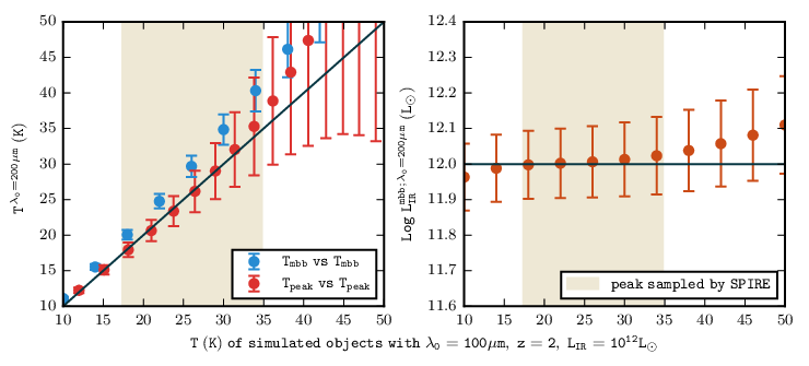
The term modifies the black body term in that it includes a wavelength-dependent optical depth , which is assumed to follow a power-law of . The parameter is the wavelength where the optical depth is unity. By default, cmcirsed sets . In this work, we followed Draine [16] and adopted .
The difference in the choice of impacts the derived significantly. This is because the “modifying” term varies significantly when different is adopted. As an example, let us consider a FIR SED that peaks at restframe . The “modifying” term is 0.63 at this peak wavelength when , but becomes 0.94 when . Therefore, in order to fit the peak flux density, the black body term will need to be smaller in the case of , which means that the derived must be smaller. For further demonstration, we generated a series of MBB models of varying using , convolved them with the SPIRE band response curves, and then fitted the simulated photometry using the MBB models with . A representative case is given in Figure 17, where the simulated objects are at and all have . The left panel shows the relation of the derived values and the input values. The peak temperature , on the other hand, will not be affected significantly because the fitting procedure, regardless of the choice of , will always find the model that best matches the given SED, and therefore the peak wavelength and the peak temperature based on the Wien’s displacement law, will not change much.
Similarly, the choice of has little impact to the derived values because the shape of the best-fit model is governed by the observed FIR SED. When its peak region is well sampled by the three SPIRE bands, the small differences in the fitted SED beyond the peak will only have a small contribution to and thus have little influence. The right panel of Figure 17 shows the comparison of based on the same simulation.
Appendix B Summary of online data table and examples of SED fitting
| Column | Name | Description |
|---|---|---|
| 1 | SDSS_IAU_name | SDSS quasar IAU name |
| 2 | Herschel_IAU_name | IAU name of the Herschel counterpart as in the original catalogs |
| 3 | str_id | Object ID assigned in this work |
| 4 | RA_250 | Herschel RA (J2000) |
| 5 | Dec_250 | Herschel Dec (J2000) |
| 6 | F250 | flux (mJy) |
| 7 | E250 | flux error (mJy) |
| 8 | F350 | flux (mJy) |
| 9 | E350 | flux error (mJy) |
| 10 | F500 | flux (mJy) |
| 11 | E500 | flux error (mJy) |
| 12 | is_SNR5 | 1: SNR in ; 0: SNR in |
| 13 | RA_100 | RA (J2000) |
| 14 | Dec_100 | Dec (J2000) |
| 15 | F100 | flux (mJy) |
| 16 | E100 | flux error (mJy) |
| 17 | RA_160 | RA (J2000) |
| 18 | Dec_160 | Dec (J2000) |
| 19 | F160 | flux (mJy) |
| 20 | E160 | flux error (mJy) |
| 21 | RA_DR7 | SDSS DR7 RA (J2000) |
| 22 | Dec_DR7 | SDSS DR7 Dec (J2000) |
| 23 | z_DR7 | SDSS DR7 redshift |
| 24 | Mi_DR7 | SDSS DR7 -band absolute magnitude (at z=0) |
| 25 | RA_DR10 | SDSS DR10 RA (J2000) |
| 26 | Dec_DR10 | SDSS DR10 Dec (J2000) |
| 27 | z_DR10 | SDSS DR10 redshift |
| 28 | Mi_DR10 | SDSS DR10 -band absolute magnitude (at z=2) |
| 29 | LOG_MBH | Black hole mass measured by Shen et al. [72] () |
| 30 | LOG_MBHERR | Error of the black hole mass |
| 31 | LOG_LX | Hard-band X-ray luminosity in the restframe () |
| 32 | GAMMA | Photon index of the X-ray SED used to derive X-ray luminosity |
| 33 | XRAY_REF | References of the X-ray data. CSC: Evans et al. [21]; 3XMM: Rosen et al. [60] |
| 34 | LOG_LIR_MBB | measured using MBB fitting (), integrated over |
| 35 | LOG_LIRERR_MBB | Error of the measured |
| 36 | CHISQ_MBB | of the MBB fitting |
| 37 | TMBB | Derived black body temperature of the best fit model (K) |
| 38 | TMBBERR | Error of (K) |
| 39 | TPEAK | Derived peak temperature of the best fit model (K) |
| 40 | LOG_MDUST | Dust mass () |
| 41 | LOG_MDUSTERR | Error of dust mass |
| 42 | LOG_SFR | SFR using Kennicutt [33], modified for Chabrier IMF () |
| 43 | LOG_MGAS | Gas mass converted from dust mass (assuming gas-to-mass-ratio of 140) |
| 44 | LOG_TDEP | Gas depletion time scale () |
| 45 | LOG_LIR_SK07 | measured using SK07 templates () |
| 46 | LOG_LIRERR_SK07 | Error of the SK07 |
| 47 | CHISQ_SK07 | of the SK07 fitting |
| 48 | LOG_LIR_CE01 | measured using CE01 templates () |
| 49 | LOG_LIRERR_CE01 | Error of the CE01 |
| 50 | CHISQ_CE01 | of the CE01 fitting |
| 51 | LOG_LIR_DH02 | measured using DH02 templates () |
| 52 | LOG_LIRERR_DH02 | Error of the DH02 |
| 53 | CHISQ_DH02 | of the DH02 fitting |

The header information of the online data table is given in Table 2. We note that this table includes all the sources as summarized in § II.3.3 and Table 1.
The SEDs and the best-fit models for the IR quasars in the SNR5 subsample are shown in Figure 18 as examples. For clarity, we only plot the MBB (red curves) and the SK07 (grey curves) model fits. While there are 134 objects in this subsample, only 102 of them have photometry in all the three SPIRE bands to allow for the MBB fit, and hence we only show these 102 objects in this figure. The other 32 objects in the SNR5 subsample still have values as determined using the starburst models (see §III), which are included in the online data table. We note that seven objects in this figure also have PACS data, for which we also have MBB+PL fits (shown as the blue curves).
Appendix C Test of AGN/Starburst decomposition

The availability of mid-to-far IR data in the recent years have allowed better characterization of AGN SEDs in this regime [74, 46, 42, 71, 44, 73, 14, e.g.]. In light of these improvements, it has been advocated that the mid-to-far IR contributions from the AGN and the host galaxy star formation can be separated through the decomposition of the SEDs [44, 14, e.g.]. Such decomposition approaches, however, still have caveats. An important one is that the AGN templates in use can only be constructed by subtracting the star formation contributions from the observed SEDs, where such contributions are determined through the calibration of some indicators of star formation activities (such as the PAH features). It is unclear whether such calibration is universally applicable given the complexity of the star forming regions. Furthermore, the far-IR part of the templates is just the extrapolation from the mid-IR part, and a cutoff has to be applied beyond a certain wavelength in FIR that is somewhat arbitrarily chosen. This means that such decomposition schemes are not appropriate to address the question of AGN contribution in FIR, because it is already assumed to be minimal by design.
With these caveats in mind, we tested the AGN and the star formation (AGN/SF) decomposition of our objects in order to further check the consistency of our conclusion that is mainly due to the heating from star formation. We only carried out this test for the objects that have the PACS data and/or those that have the Spitzer MIPS 24/ data readily available from the releases of the relevant Spitzer Legacy Survey programs residing in the IPAC Infrared Science Archinve (IRSA). In brief, there are in total 87 (COSMOS 33, Lockman 26, FLS 14, XMM-LSS-SWIRE 14) objects in our IR quasar sample that have at least MIPS data, among which 37 objects have detections in all the three SPIRE bands, and thus are suitable for the test and the comparison.
We used the software suite of Mullaney et al. [44] in this test. This particular flavor of decomposition involves one AGN template and five starburst templates (denoted from “SB1” to “SB5”), and in each fitting run the routine combines the AGN template and one of the five starburst templates and determines the normalizations through the least- fitting. The AGN template is forced to cut off at a wavelength between 20 and in the form of a black body, and the exact cut-off wavelength is determined during the fitting. The exact AGN+SB combination that gave the smallest was deemed to be the best fit, from which the total IR luminosities (integrating over ) due to the AGN and the SB heating were then obtained. Here we denote these as and , respectively, and denote the fraction of the AGN contribution as . Figure 19 compares thus obtained to (filled red circles) and (open blue circles) that we derived based on the fit to the SPIRE data as described in §III and §IV. The mean difference between () and is () with a sample standard deviation (). The results are fully consistent with what we derived using solely the SPIRE bands, i.e., and , which both measure the total IR luminosity due to star formation, agree to within , while , which measures only the total IR luminosity from the cold-dust component, is less than by . Considering the differences in the methods and the template sets employed, we conclude that the decomposition test also provides results that are consistent with our interpretation that is mainly due to the heating of star formation.
Appendix D Stacking analysis of Herschel-undetected SDSS quasars
To investigate how the survey limits impact our results, we performed a stacking analysis of the SDSS quasars that are not matched in the adopted HerMES, H-ATLAS and HerS catalogs. While a fraction of these unmatched SDSS quasars could be blended sources rejected by our stringent matching criterion, the majority should be those that are undetected in the current SPIRE data. It is difficult to stack all such objects from all fields, because different fields have different survey sensitivities. Therefore, we only stacked on a field-by-field basis. We show here the results in the HerMES L6-XMM-LSS and L5-Bootes fields and the HerS field, which are representative of the entire data sets in terms of survey limit.
D.1. Stacking procedure and photometry

The unmatched SDSS quasars in each field were first split into different bins by redshifts. For simplicity, we only discuss the “equal redshift” case but not the “equal volume” one. We adopted a large step-size, , to ensure enough number of objects for stacking at the most critical redshifts. The objects were then visually inspected in and were subsequently divided into three categories: “weak” objects seem to have some weak enhancement at the source locations, “invisible” objects do not have any sign of detection, and “contaminated” objects are likely contaminated by nearby sources. The results from this classification, while done in , were assumed to be valid in 350 and as well. The detailed numbers are listed in Table 3 for these three fields. The stacking was done for these three categories separately in each redshift bin, using both average and median as the combining methods. We also combined the “invisible” and the “weak” objects into the “combined” set and stacked them together. In most cases, the “invisible” stacks still do not result in significant detections, while the “weak” stacks usually result in positive detections in at least 250 and . The “combined” stacks, on the other hand, are weaker than the “weak” stacks, but are still positive detections in at least . The “contaminated” stacks, as expected, often show contamination from the residuals of the blended neighbors, and hence were excluded from further discussion. For demonstration, Figure 20 shows the average and the median stacks in these four cases for the quasars at in the L6-XMM-LSS-SWIRE field.
We used the Herschel Interactive Processing Environment (HIPE) software package to do photometry on the stacks. The Herschel science and uncertainty frames of the image cutouts at the undetected SDSS quasar coordinates were stacked separately and inputted to HIPE task sourceExtractorSussextractor, which then performed PSF fitting to measure the fluxes and associated errors. A detection limit was adopted during the photometry. The measured results are also listed in Table 3.
As the “invisible” set usually does not result in detections, it will not be discussed further as an independent set. We will focus on the “weak” and the “comb” sets.
| invisible set | weak set | combined set | ||||||||||
|---|---|---|---|---|---|---|---|---|---|---|---|---|
| z | ||||||||||||
| Bootes-HerMES | ||||||||||||
| (0, 1] | 24 | – | – | – | 10 | – | 34 | – | ||||
| – | – | – | – | – | – | |||||||
| (1, 2] | 21 | – | – | – | 15 | 36 | ||||||
| – | – | |||||||||||
| (2, 3] | 66 | – | – | – | 22 | 88 | – | – | ||||
| – | – | – | – | |||||||||
| (3, 4] | 21 | – | – | – | 4 | 25 | – | – | ||||
| – | – | – | – | – | ||||||||
| (4, 5] | 2 | – | – | 0 | – | – | – | 2 | – | – | ||
| – | – | – | – | – | – | – | ||||||
| XMM-LSS-SWIRE | ||||||||||||
| (0, 1] | 31 | – | – | – | 12 | 43 | – | – | ||||
| – | – | – | – | – | ||||||||
| (1, 2] | 10 | – | – | – | 8 | – | 18 | – | – | |||
| – | – | – | – | – | ||||||||
| (2, 3] | 113 | – | – | – | 41 | 154 | – | |||||
| – | – | |||||||||||
| (3, 4] | 18 | – | – | 7 | 25 | – | – | |||||
| – | – | – | – | |||||||||
| (4, 5] | 1 | – | – | 0 | – | – | – | 1 | – | – | – | |
| – | – | – | – | – | – | – | – | |||||
| HerS | ||||||||||||
| (0, 1] | 904 | 0 | – | – | – | 904 | ||||||
| – | – | – | ||||||||||
| (1, 2] | 699 | – | – | – | 452 | 1151 | ||||||
| – | – | – | ||||||||||
| (2, 3] | 1046 | – | – | – | 350 | 1396 | ||||||
| – | – | – | ||||||||||
| (3, 4] | 220 | – | – | – | 77 | 297 | ||||||
| – | – | – | – | |||||||||
| (4, 5] | 27 | – | – | – | 0 | – | – | – | 27 | – | – | – |
| – | – | – | – | – | – | – | – | – | ||||
D.2. IR luminosity
The FIR SEDs of the stacks could be fit in the usual way. There is a caveat, however. The implicit assumption of any stacking analysis is always that the sources being stacked can be scaled linearly. This is not necessary true in our case, because these Herschel-undetected SDSS quasars could be of different dust temperatures and hence their intrinsic FIR SEDs could vary significantly in shape. Therefore, the physical properties inferred from the SED fitting of the stacks should be interpreted with caution. Here we only focus on the total IR luminosities of the stacks, and assume that these are the representative values of the stacked population.
In most cases, only the stacks have detections of sufficient S/N, and this prevented us from doing the full suite of FIR SED fitting as in §III. First of all, we had to abandon the MBB fit because it would require at least three bands to obtain reasonable constraints. This left the three starburst models to use, which all allow the estimation of by searching for the template whose associated is the closest match to the one or two-band flux densities at the given redshift. However, we also opted to abandon the SK07 models because in some cases the results had large discrepancies with respect to those based on CE01 and DH02. This is largely due to the wide dynamic range and the fine grid of the SK07 templates, which could make their results highly degenerated in case when only one or two bands are available. As we only have a very limited number of bins here, including these deviant SK07 results would significantly skew the picture. Therefore, we used the results from the CE01 and the DH02 templates for this analysis. These results are summarized in Table 4.
| weak set | combined set | |||||||
| Bootes-HerMES | ||||||||
| 10 | 15 | 22 | 4 | 34 | 36 | 88 | 25 | |
| 11.5 (11.5*) | 12.0 (12.0) | 12.2 (12.3) | 12.8 (12.7) | 11.2 (11.2*) | 11.5 (11.6) | 11.5*(11.5) | 12.2*(12.2*) | |
| 11.4 (11.4*) | 12.0 (12.2) | 12.2 (12.2) | 12.8 (12.6) | 11.2 (11.2*) | 11.4 (11.7) | 11.4*(11.7) | 12.2*(12.2*) | |
| XMM-LSS-SWIRE | ||||||||
| 12 | 8 | 41 | 7 | 43 | 18 | 154 | 25 | |
| 11.6 (11.5) | 12.1 (12.1) | 12.3 (12.3) | 12.6 (12.7) | 10.5*(11.6*) | 11.8*(11.8) | 11.7 (11.8) | 12.1*(12.2) | |
| 11.4 (11.4) | 12.2 (12.2) | 12.4 (12.2) | 12.6 (12.6) | 10.6*(11.2*) | 11.7*(11.7) | 11.7 (11.7) | 12.0*(12.2) | |
| HerS | ||||||||
| 452 | 350 | 77 | 1151 | 1396 | 297 | |||
| 12.2 (12.2) | 12.6 (12.6) | 12.7 (12.8) | 11.8 (11.9) | 12.0 (12.0) | 12.3 (12.3) | |||
| 12.2 (12.2) | 12.6 (12.6) | 12.8 (12.8) | 12.0 (12.0) | 12.0 (12.0) | 12.4 (12.2) | |||
D.3. Correction to fraction of IR-luminous quasars
One key objective of this stacking analysis was to study how the distribution of the fraction of IR-luminous optical quasars (see Figure 15) will change if the undetected population is taken into account. In particular, we are interested in understanding whether the sharp drop from to higher redshifts is caused by the potential bias when using only the SPIRE-detected objects for the statistics.
This IR-luminous fraction depends on the exact choice of , which could be below the survey limit of the data, and therefore ideally we should compensate for the number of objects that are below the survey limit and yet still have . However, as Table 4 shows, this is not always possible because we cannot control the input undetected objects so that they will stack to the exact required. Therefore, we need to make corrections in a different way.
As we have chosen , it is only necessary to analyze the “weak” sets, because from Table 4 it is obvious that the individually undetected objects that still have can only be found in these sets. We first start from the bin. In the L5-Boötes field, there are 18 SPIRE-detected quasars in this bin that have . The stack of 22 undetected objects in this bin, on the other hand, has the median of from the fits using CE01 or DH02 models. We use the superscript “” to denoted that this quantity is for the “undetected” objects. By the definition of median, half (i.e., 11) of these undetected objects should have . As , we conclude that at most there are 11 objects that can be added to the existing 18 objects. In other words, the number of objects above the threshold after this correction, , should be , and the correction factor, , should be . Similarly, for the bin of , there are 5 objects that have , and the stack of 15 undetected objects has the median of . Therefore we get , and .
We can repeat the similar analysis for all the fields, and obtain the constrained corrections for each redshift bin. If , such a correction is “maximum possible”, and if , such a correction is “minimum necessary”. At , the corrections are all “maximum possible”. At , the correction is “minimum necessary” for the HerS field, and are “maximum possible” for all other fields. However, the HerS field dominates the statistics here at : the stack of 350 Herschel-undetected quasars has median , which means that we need to add 175 objects for the correction by this field alone. The total number of Herschel-detected quasars that have in this redshift bin is 84, and if we ignore the “maximum possible” corrections in other fields, the “minimum necessary” corrections will be at least for the entire sample.
D.4. Correction to IR luminosity density
As expected, the Herschel-undetected SDSS quasars are significantly less luminous than the Herschel-detected ones at the same redshifts. However, their collective contributions to are comparable to those from the Herschel-detected population, simply because of their larger number. This is particularly true at , where their contribution is even higher by a factor of .
The correction in each redshift bin was done by adding the product of the average stacked values of the “combined” sets multiplied by the number of input objects in these sets. After such corrections, the evolution of will peak at instead of .
References
- [1] Aaronson, M., & Olszewski, E. W. 1984, Nature, 309, 414
- [2] Abazajian, K. N., Adelman-McCarthy, J. K., Agüeros, M. A., et al. 2009, ApJS, 182, 543
- [3] Annis, J., Soares-Santos, M., Strauss, M. A., et al. 2014, ApJ, 794, 120
- [4] Azadi, M., Aird, J., Coil, A. L., et al. 2015, ApJ, 806, 187
- [5] Blain, A. W., Smail, I., Ivison, R. J., Kneib, J.-P., & Frayer, D. T. 2002, Phys. Rep., 369, 111
- [6] Bovy, J., Hennawi, J. F., Hogg, D. W., et al. 2011, ApJ, 729, 141
- [7] Cao, C., Xia, X. Y., Wu, H., et al. 2008, MNRAS, 390, 336
- [8] Carter, D. 1984, Astronomy Express, 1, 61
- [9] Casey, C. M. 2012, MNRAS, 425, 3094
- [10] Chary, R., & Elbaz, D. 2001, ApJ, 556, 562
- [11] Daddi, E., Dickinson, M., Chary, R., et al. 2005, ApJ, 631, L13
- [12] Dai, Y. S., Bergeron, J., Elvis, M., et al. 2012, ApJ, 753, 33
- [13] Dale, D. A., & Helou, G. 2002, ApJ, 576, 159
- [14] Dale, D. A., Helou, G., Magdis, G. E., et al. 2014, ApJ, 784, 83
- [15] de Grijp, M. H. K., Miley, G. K., Lub, J., & de Jong, T. 1985, Nature, 314, 240
- [16] Draine, B. T. 2006, ApJ, 636, 1114
- [17] Draine, B. T., Dale, D. A., Bendo, G., et al. 2007, ApJ, 663, 866
- [18] Eales, S., Dunne, L., Clements, D., et al. 2010, PASP, 122, 499
- [19] Elston, R., Cornell, M. E., & Lebofsky, M. J. 1985, ApJ, 296, 106
- [20] Evans, A. S., Frayer, D. T., Surace, J. A., & Sanders, D. B. 2001, AJ, 121, 1893
- [21] Evans, I. N., Primini, F. A., Glotfelty, K. J., et al. 2010, ApJS, 189, 37
- [22] González-Nuevo, J., de Zotti, G., Andreani, P., et al. 2010, A&A, 518, L38
- [23] Griffin, M. J., Abergel, A., Abreu, A., et al. 2010, A&A, 518, L3
- [24] Haas, M., Klaas, U., Müller, S. A. H., et al. 2003, A&A, 402, 87
- [25] Hao, L., Weedman, D. W., Spoon, H. W. W., et al. 2007, ApJ, 655, L77
- [26] Heckman, T. M., Armus, L., & Miley, G. K. 1987, AJ, 93, 276
- [27] Hopkins, A. M., & Beacom, J. F. 2006, ApJ, 651, 142
- [28] Houck, J. R., Schneider, D. P., Danielson, G. E., et al. 1985, ApJ, 290, L5
- [29] Houck, J. R., Soifer, B. T., Neugebauer, G., et al. 1984, ApJ, 278, L63
- [30] Ibar, E., Ivison, R. J., Cava, A., et al. 2010, MNRAS, 409, 38
- [31] Ivison, R. J., Greve, T. R., Dunlop, J. S., et al. 2007, MNRAS, 380, 199
- [32] Jiang, L., Fan, X., Cool, R. J., et al. 2006, AJ, 131, 2788
- [33] Kennicutt, Jr., R. C. 1998, ARA&A, 36, 189
- [34] Kim, D.-C., & Sanders, D. B. 1998, ApJS, 119, 41
- [35] Lawrence, A., Rowan-Robinson, M., Ellis, R. S., et al. 1999, MNRAS, 308, 897
- [36] Leipski, C., Meisenheimer, K., Klaas, U., et al. 2010, A&A, 518, L34
- [37] Leipski, C., Meisenheimer, K., Walter, F., et al. 2013, ApJ, 772, 103
- [38] —. 2014, ApJ, 785, 154
- [39] Lonsdale, C. J., Farrah, D., & Smith, H. E. 2006, Ultraluminous Infrared Galaxies, ed. J. W. Mason, 285
- [40] Lutz, D., Poglitsch, A., Altieri, B., et al. 2011, A&A, 532, A90
- [41] Magnelli, B., Elbaz, D., Chary, R. R., et al. 2009, A&A, 496, 57
- [42] Maiolino, R., Shemmer, O., Imanishi, M., et al. 2007, A&A, 468, 979
- [43] Massaro, E., Giommi, P., Leto, C., et al. 2009, A&A, 495, 691
- [44] Mullaney, J. R., Alexander, D. M., Goulding, A. D., & Hickox, R. C. 2011, MNRAS, 414, 1082
- [45] Netzer, H., Mor, R., Trakhtenbrot, B., Shemmer, O., & Lira, P. 2014, ApJ, 791, 34
- [46] Netzer, H., Lutz, D., Schweitzer, M., et al. 2007, ApJ, 666, 806
- [47] Oliver, S. J., Bock, J., Altieri, B., et al. 2012, MNRAS, 424, 1614
- [48] Osmer, P. S. 2004, Coevolution of Black Holes and Galaxies, 324
- [49] Osterbrock, D. E., & De Robertis, M. M. 1985, PASP, 97, 1129
- [50] Pâris, I., Petitjean, P., Aubourg, É., et al. 2014, A&A, 563, A54
- [51] Pascale, E., Auld, R., Dariush, A., et al. 2011, MNRAS, 415, 911
- [52] Pilbratt, G. L., Riedinger, J. R., Passvogel, T., et al. 2010, A&A, 518, L1
- [53] Poglitsch, A., Waelkens, C., Geis, N., et al. 2010, A&A, 518, L2
- [54] Pope, A., & Chary, R.-R. 2010, ApJ, 715, L171
- [55] Richards, G. T., Fan, X., Newberg, H. J., et al. 2002, AJ, 123, 2945
- [56] Richards, G. T., Strauss, M. A., Fan, X., et al. 2006, AJ, 131, 2766
- [57] Riechers, D. A., Bradford, C. M., Clements, D. L., et al. 2013, Nature, 496, 329
- [58] Rigby, E. E., Maddox, S. J., Dunne, L., et al. 2011, MNRAS, 415, 2336
- [59] Roseboom, I. G., Oliver, S. J., Kunz, M., et al. 2010, MNRAS, 409, 48
- [60] Rosen, S. R., Webb, N. A., Watson, M. G., et al. 2015, ArXiv e-prints, arXiv:1504.07051
- [61] Ross, N. P., Myers, A. D., Sheldon, E. S., et al. 2012, ApJS, 199, 3
- [62] Ross, N. P., McGreer, I. D., White, M., et al. 2013, ApJ, 773, 14
- [63] Rowan-Robinson, M. 1995, MNRAS, 272, 737
- [64] Rowan-Robinson, M., Lari, C., Perez-Fournon, I., et al. 2004, MNRAS, 351, 1290
- [65] Sanders, D. B., Phinney, E. S., Neugebauer, G., Soifer, B. T., & Matthews, K. 1989, ApJ, 347, 29
- [66] Sanders, D. B., Soifer, B. T., Elias, J. H., et al. 1988, ApJ, 325, 74
- [67] Schneider, D. P., Richards, G. T., Hall, P. B., et al. 2010, AJ, 139, 2360
- [68] Schweitzer, M., Lutz, D., Sturm, E., et al. 2006, ApJ, 649, 79
- [69] Scoville, N. Z., Frayer, D. T., Schinnerer, E., & Christopher, M. 2003, ApJ, 585, L105
- [70] Serjeant, S., Bertoldi, F., Blain, A. W., et al. 2010, A&A, 518, L7
- [71] Shang, Z., Brotherton, M. S., Wills, B. J., et al. 2011, ApJS, 196, 2
- [72] Shen, Y., Richards, G. T., Strauss, M. A., et al. 2011, ApJS, 194, 45
- [73] Shi, Y., Helou, G., Armus, L., Stierwalt, S., & Dale, D. 2013, ApJ, 764, 28
- [74] Shi, Y., Ogle, P., Rieke, G. H., et al. 2007, ApJ, 669, 841
- [75] Siebenmorgen, R., & Krügel, E. 2007, A&A, 461, 445
- [76] Smith, D. J. B., Dunne, L., Maddox, S. J., et al. 2011, MNRAS, 416, 857
- [77] Solomon, P. M., & Vanden Bout, P. A. 2005, ARA&A, 43, 677
- [78] Symeonidis, M., Vaccari, M., Berta, S., et al. 2013, MNRAS, 431, 2317
- [79] Symeonidis, M., Georgakakis, A., Page, M. J., et al. 2014, MNRAS, 443, 3728
- [80] Viero, M. P., Moncelsi, L., Quadri, R. F., et al. 2013, ApJ, 779, 32
- [81] Viero, M. P., Asboth, V., Roseboom, I. G., et al. 2014, ApJS, 210, 22
- [82] Wang, L., Viero, M., Clarke, C., et al. 2013, ArXiv e-prints, arXiv:1312.0552
- [83] Wang, R., Carilli, C. L., Neri, R., et al. 2010, ApJ, 714, 699
- [84] Wang, R., Wagg, J., Carilli, C. L., et al. 2011a, ApJ, 739, L34
- [85] —. 2011b, AJ, 142, 101
- [86] Xia, X. Y., Gao, Y., Hao, C.-N., et al. 2012, ApJ, 750, 92
- [87] Yan, H., Stefanon, M., Ma, Z., et al. 2014, ApJS, 213, 2
- [88] York, D. G., Adelman, J., Anderson, Jr., J. E., et al. 2000, AJ, 120, 1579