跳到论文正文
W Papers独立论文阅读器 arXiv:1501.00438 论文正文 计算阅读时间 · 0%
引用这篇论文根据当前论文元数据生成,正式投稿前建议核对。


License: arXiv.org perpetual non-exclusive license
arXiv:1501.00438v2 [stat.ME] 21 Sep 2015

Exploration of the (Non-)asymptotic Bias and Variance of Stochastic Gradient Langevin Dynamics

Sebastian J. Vollmer ††thanks: vollmer@stats.ox.ac.uk Affiliation: Department of Statistics, University of Oxford    Konstantinos C. Zygalakis ††thanks: k.zygalakis@soton.ac.uk Affiliation: Mathematical Sciences, University of Southampton.    Yee Whye Teh ††thanks: y.w.teh@stats.ox.ac.uk Affiliation: Department of Statistics, University of Oxford

Applying standard Markov chain Monte Carlo (MCMC) algorithms to large data sets is computationally infeasible. The recently proposed stochastic gradient Langevin dynamics (SGLD) method circumvents this problem in three ways: it generates proposed moves using only a subset of the data, it skips the Metropolis-Hastings accept-reject step, and it uses sequences of decreasing step sizes. In [Teh et al., 2014], we provided the mathematical foundations for the decreasing step size SGLD, including consistency and a central limit theorem. However, in practice the SGLD is run for a relatively small number of iterations, and its step size is not decreased to zero. The present article investigates the behaviour of the SGLD with fixed step size. In particular we characterise the asymptotic bias explicitly, along with its dependence on the step size and the variance of the stochastic gradient. On that basis a modified SGLD which removes the asymptotic bias due to the variance of the stochastic gradients up to first order in the step size is derived. Moreover, we are able to obtain bounds on the finite-time bias, variance and mean squared error (MSE). The theory is illustrated with a Gaussian toy model for which the bias and the MSE for the estimation of moments can be obtained explicitly. For this toy model we study the gain of the SGLD over the standard Euler method in the limit of large data sets.

Keywords: Markov Chain Monte Carlo, Langevin Dynamics, Big Data, Fixed step size

1 Introduction

A standard approach to estimating expectations under a given target density π⁡(θ)\pi(\theta) is to construct and simulate from Markov chains whose equilibrium distributions are designed to be π\pi [Brooks et al., 2011b]. A well-studied approach, for example in molecular dynamics [Leimkuhler and Matthews, 2013, Bou-Rabee and Vanden-Eijnden, 2010] and throughout Bayesian statistics [Milstein and Tretyakov, 2007, Neal, 2011], is to use Markov chains constructed as numerical schemes which approximate the time dynamics of stochastic differential equations (SDEs). In this paper we will focus on the case of first order Langevin dynamics, which has the form

dθ(t)=12∇logπ(θ(t))dt+dWt,d\theta(t)=\frac{1}{2}\nabla\log{\pi(\theta(t))}dt+dW_{t}, (1)

where t∈ℝ+t\in\mathbb{R}_{+}, θ∈ℝd\theta\in\mathbb{R}^{d} and WtW_{t} is a dd-dimensional standard Brownian motion. Under appropriate assumptions on π⁡(θ)\pi(\theta), it is possible to show that the dynamics generated by Equation (1) are ergodic with respect to π⁡(θ)\pi(\theta).

The simplest possible numerical scheme for approximating Equation (1) is the Euler-Maruyama method. Let h>0h>0 be a step size. Abusing notation, the diffusion θ⁡(k⋅h)\theta(k\cdot h) at time k⋅hk\cdot h is approximated by θk\theta_{k}, which is obtained using the following recursion equation

θk+1=θk+h2∇logπ(θk)+hξk,\theta_{k+1}=\theta_{k}+\frac{h}{2}\nabla\log\pi(\theta_{k})+\sqrt{h}\xi_{k}, (2)

where ξk\xi_{k} is a standard Gaussian random variable on ℝd\mathbb{R}^{d}. One can use the numerical trajectories generated by this scheme for the construction of an empirical measure πh​(θ)\pi_{h}(\theta) either by averaging over one single long trajectory or by averaging over many realisations in order to obtain a finite ensemble average (see for example [Milstein and Tretyakov, 2007]). However, as discussed in [Roberts and Tweedie, 1996], one needs to be careful when doing this as it could be the case that the discrete Markov chain generated by Equation (2) is not ergodic. But even if the resulting Markov Chain is ergodic, πh​(θ)\pi_{h}(\theta) will not be equal to π⁡(θ)\pi(\theta) [Mattingly et al., 2010, Abdulle et al., 2014] which thus implies that the resulting sample average is biased. An alternative strategy that avoids this discretization bias and the ergodicity of the numerical procedure, is to use Equation (2) as a proposal for a Metropolis-Hastings (MH) MCMC algorithm [Brooks et al., 2011a], with an additional accept-reject step which corrects the discretization error.

In this paper we are interested in situations where π\pi arises as the posterior in a Bayesian inference problem with prior density π0​(θ)\pi_{0}(\theta) and a large number N≫1N\gg 1 of i.i.d. observations XiX_{i} with likelihoods π⁡(Xi|θ)\pi(X_{i}|\theta). In this case, we can write

π⁡(θ)∝π0​(θ)​∏i=1Nπ⁡(Xi|θ),\pi(\theta)\propto\pi_{0}(\theta)\prod_{i=1}^{N}\pi(X_{i}|\theta), (3)

and we have the following gradient,

∇log⁡π​(θ)=∇log⁡π0​(θ)+∑i=1N∇log⁡π​(Xi|θ).\nabla\log{\pi(\theta)}=\nabla\log{\pi_{0}(\theta)}+\sum_{i=1}^{N}\nabla\log{\pi(X_{i}|\theta)}. (4)

In these situations each update (2) has an impractically high computational cost of 𝒪⁡(N)\mathcal{O}(N) since it involves computations on all NN items in the dataset. Likewise, each MH accept-reject step is impractically expensive.

In contrast, the recently proposed stochastic gradient Langevin dynamics (SGLD) [Welling and Teh, 2011] circumvents this problem by generating proposals which are only based on a subset of the data, by skipping the accept-reject step and by using a decreasing step-size sequence (hk)k≥0(h_{k})_{k\geq 0}. In particular one has

θk+1\displaystyle\theta_{k+1} =θk+hk2​∇log⁡π^​(θk)+hk​ξk,\displaystyle=\theta_{k}+\frac{h_{k}}{2}\widehat{\nabla\log{\pi}}(\theta_{k})+\sqrt{h_{k}}\xi_{k}, (5)
∇log⁡π^​(θk)\displaystyle\widehat{\nabla\log{\pi}}(\theta_{k}) =∇log⁡π0​(θk)+Nn​∑i=1n∇log⁡π​(Xτk​i|θk)\displaystyle=\nabla\log{\pi_{0}(\theta_{k})}+\frac{N}{n}\sum_{i=1}^{n}\nabla\log{\pi(X_{\tau_{ki}}|\theta_{k})} (6)

where ξk\xi_{k} are independent standard Gaussian random variables on ℝd\mathbb{R}^{d}, and τk=(τk​1,⋯,τk​n)\tau_{k}=(\tau_{k1},\cdots,\tau_{kn}) is a random subset of [N]:={1,⋯,N}[N]:=\{1,\cdots,N\} of size nn, generated, for example, by sampling with or without replacement from [N][N]. The idea behind this algorithm is that, since the stochastic gradient appearing in Equation (5) is an unbiased estimator of the true gradient ∇log⁡π​(θ)\nabla\log{\pi(\theta)}, the additional perturbation due to the gradient stochasticity is of order hh, smaller than the h\sqrt{h} order of the injected noise, and so the limiting dynamics (k→∞k\rightarrow\infty) of Equation (5) should behave similarly to the case n=Nn=N. In [Teh et al., 2014] it was shown that in this case that the KK-step size weighted sample average is consistent and satisfies a CLT with rate depending on the decay of hkh_{k}. The optimal rate is limited to K−13K^{-\frac{1}{3}} and achieved by an asymptotic step size decay of ≍K−13\asymp K^{-\frac{1}{3}}.

The problem with decaying step sizes is that the efficiency of the algorithm slows the longer it is run for. A common practice for the SGLD and its extensions, the Stochastic Gradient Hamiltonian Monte Carlo [Chen et al., 2014] and the Stochastic Gradient Thermostat Monte Carlo algorithm [Ding et al., 2014], is to use step sizes that are only decreasing up to a point. The primary aim of this paper is to analyse the behaviour of SGLD with fixed step sizes of hk=hh_{k}=h. We provide two complementary analyses in this setting, one asymptotic in nature and one finite time. Let ϕ:ℝd→ℝ\phi:\mathbb{R}^{d}\rightarrow\mathbb{R} be a test function whose expectation we are interested in estimating. Using simulations of the dynamics governed by Equation (5), we can estimate the expectation using

𝔼π​[ϕ⁡(θ)]≈1K​∑k=1Kϕ⁡(θk)\mathbb{E}_{\pi}[\phi(\theta)]\approx\frac{1}{K}\sum_{k=1}^{K}\phi(\theta_{k}) (7)

for some large number of steps KK. Our analyses shed light on the behaviour of this estimator.

In the first analysis, we are interested in the asymptotic bias of the estimator (7) as K→∞K\rightarrow\infty,

limK→∞1K​∑k=1Kϕ⁡(θk)−𝔼π​[ϕ⁡(θ)].\lim_{K\rightarrow\infty}\frac{1}{K}\sum_{k=1}^{K}\phi(\theta_{k})-\mathbb{E}_{\pi}[\phi(\theta)]. (8)

Assuming for the moment that the dynamics governed by Equation (5) is ergodic, with invariant measure πh​(θ,n)\pi_{h}(\theta;n), the above asymptotic bias simply becomes 𝔼πh​(⋅,n)​[ϕ⁡(θ)]−𝔼π​[ϕ⁡(θ)]\mathbb{E}_{\pi_{h}(\cdot;n)}[\phi(\theta)]-\mathbb{E}_{\pi}[\phi(\theta)]. In the case of Euler-Maruyama, where n=Nn=N and the gradient is computed exactly, the asymptotic behaviour of the dynamics is well understood, in particular its asymptotic bias is 𝒪⁡(h)\mathcal{O}(h) [Mattingly et al., 2010]. When n<Nn<N, using the recent generalisations [Abdulle et al., 2014, Sato and Nakagawa, 2014] of the approach by [Talay and Tubaro, 1990] reviewed in Section 3, we are able to derive an expansion of the asymptotic bias in powers of the step size hh. This allows us to explicitly identify the effect, on the leading order term in the asymptotic bias, of replacing the true gradient (4) with the unbiased estimator (6). In particular, we show in Section 4 that, relative to Euler-Maruyama, the leading term contains an additional factor related to the covariance of the subsampled gradient estimators (6).

Based on this result, in Section 4.2, we propose a modification of the SGLD (referred to simply as mSGLD) which has the same asymptotic bias as the Euler-Maruyama method up to first order in hh. The mSGLD is given by

θk+1=θk+h2​∇log⁡π^​(θk)+h​(I−h2​Cov​[∇log⁡π^​(θk)])​ξj\theta_{k+1}=\theta_{k}+\frac{h}{2}\widehat{\nabla\log{\pi}}(\theta_{k})+\sqrt{h}\left(I-\frac{h}{2}\text{Cov}\left[\widehat{\nabla\log{\pi}}(\theta_{k})\right]\right)\xi_{j} (9)

where Cov​[∇log⁡π^​(θk)]\text{Cov}\left[\widehat{\nabla\log{\pi}}(\theta_{k})\right] is the covariance of the gradient estimator. When the covariance is unknown, it can in turn be estimated by subsampling as well. This modification is different from the Stochastic Gradient Fisher Scoring [S. Ahn and Welling, 2012], a modification of the injected noise in order to better match the Bernstein von Mises posterior. In contrast, the mSGLD is a local modification based on the estimated variance of the stochastic gradient.

The second contribution provides a complementary finite time analysis. In the finite time case both the bias and the variance of the estimator are non-negligible, and our analysis accounts for both by focussing on bounding the mean squared error (MSE) of the estimator (7). Our results, presented in Section 5, show that,

𝔼⁡[(1K​∑k=0K−1ϕ⁡(θk)−π⁡(ϕ))2]≤C⁡(n)​(h2+1K​h),\mathbb{E}\left[\left(\frac{1}{K}\sum_{k=0}^{K-1}\phi(\theta_{k})-\pi(\phi)\right)^{2}\right]\leq C(n)\left(h^{2}+\frac{1}{Kh}\right), (10)

where the RHS only depends on nn through the constant C⁡(n)C(n), the h2h^{2} term is a contribution of the (square of the) bias while the 1/K​h1/Kh term is a contribution of the variance. We see that there is a bias-variance trade-off, with bias increasing and variance decreasing monotonically with hh. Intuitively, with larger hh the Markov chain can converge faster (lower variance) with the same number of steps, but this incurs higher discretization error. Our result is achieved by extending the work of [Mattingly et al., 2010] from 𝕋d\mathbb{T}^{d} to ℝd\mathbb{R}^{d}. The main difficulty in achieving this relates to combining the results of [Pardoux and Veretennikov, 2001] and [Teh et al., 2014], in order to establish the existence of nice, well controlled solutions to the corresponding Poisson equation [Mattingly et al., 2010]. We can minimise Equation (10) over hh, finding that the minimizing hh is on the order of K−13K^{-\frac{1}{3}}, and yields an MSE of order K−23K^{-\frac{2}{3}}. This agrees, surprisingly, with the scaling of K−13K^{-\frac{1}{3}} for the central limit theorem established for the case of decreasing step sizes, for the Euler-Maruyama scheme in [Lamberton and Pages, 2002] and for SGLD in [Teh et al., 2014]. This unexpected result, that the decreasing step size and fixed step size discretisations have, up to a constant, the same efficiency seems to be missing from the literature.

Our theoretical findings are confirmed by numerical simulations. More precisely, we start by studying a one dimensional Gaussian toy model both in terms of the asymptotic bias and the MSE of time averages in Section 2. The simplicity of this model allows us to obtain explicit expressions for these quantities and thus illustrate in a clear way the connection with the theory. More precisely, we confirm that the scaling of the step size and the number of steps for a prescribed MSE obtained from the upper bound in Equation (10) matches the scaling derived from the analytic expression for the MSE for this toy model. More importantly, this simplicity allows us to make significant analytic progress in the study of the asymptotic bias and MSE of time averages in the limit of large data sets N→∞N\rightarrow\infty. In particular, we are able to show that the SGLD reduces the computational complexity by one order of magnitude in NN. for the estimation of the second moment in comparison with the Euler method if the error is quantified through the MSE.

In summary, this paper is organised as follows. We present our first explorations of the SGLD applied to a one-dimensional Gaussian toy model in Section 2. For this model we obtain an analytic characterisation of its bias and variance. This serves as intuition and benchmark for the two analyses developed in Sections 3 to 5. In Section 3 we review some known results about the effect of the numerical discretisation of Equation (1) in terms of the finite time weak error as well as in terms of the invariant measure approximation. In Section 4 we apply these results to analyse the finite and long time properties of the SGLD, as well as to construct the modified SGLD algorithm which, asymptotically in hh, behaves exactly as the Euler-Maruyama method (n=Nn=N) while still sub-sampling the data set at each step. Furthermore, in Section 5 we discuss the properties of the finite time sample averages, include its MSE. In Section 6 we revisit the Gaussian toy model to obtain a more precise understanding of the behaviour of SGLD in a large data and high accuracy regime. This is achieved using analytic expressions of the expectations of the sample average which are obtained using the supplemented Mathematica® notebook described in detail in Appendix 10. Finally, in Section 7 we demonstrate the observed performance of SGLD for a Bayesian logistic regression model which matches the theory, while, we conclude this paper in Section 8 with a discussion on some possible extensions of this work.

2 Exploring a one-dimensional Gaussian Toy Model

In this section, we develop results for a simple toy model, which will serve as a benchmark for the theory developed in Sections 3 to 5. In particular, we obtain analytic expressions for the bias and the variance of the sample average of the SGLD, allowing us to characterise its performance in detail.

We consider a one-dimensional linear Gaussian model,

θ∼𝒩⁡(0,σθ2),Xi|θ∼i.i.d.𝒩⁡(θ,σx2)for i=1,…,N.\displaystyle\begin{aligned} \theta&\sim\mathcal{N}(0,\sigma_{\theta}^{2}),\\ X_{i}\,|\,\theta&\stackrel{{\scriptstyle i.i.d.}}{{\sim}}\mathcal{N}(\theta,\sigma_{x}^{2})&&\text{for $i=1,\ldots,N$.}\end{aligned} (11)

The posterior is given by

π=𝒩⁡(μp,σp2)=𝒩⁡(∑i=1NXiσx2σθ2+N,(1σθ2+Nσx2)−1).\pi=\mathcal{N}(\mu_{p},\sigma_{p}^{2})=\mathcal{N}\left(\frac{\sum_{i=1}^{N}X_{i}}{\frac{\sigma_{x}^{2}}{\sigma_{\theta}^{2}}+N},\left(\frac{1}{\sigma_{\theta}^{2}}+\frac{N}{\sigma_{x}^{2}}\right)^{-1}\right). (12)

For this choice of π\pi, the Langevin diffusion (1) becomes,

d​θ​(t)=−12​(θ⁡(t)−μpσp2)​d​t+d​Wt,d\theta(t)=-\frac{1}{2}\left(\frac{\theta(t)-\mu_{p}}{\sigma_{p}^{2}}\right)dt+dW_{t}, (13)

and its numerical discretisation by the SGLD with step size hh reads as follows,

θk+1=(1−A​h)​θk+Bk​h+h​ξk,\theta_{k+1}=(1-Ah)\theta_{k}+B_{k}h+\sqrt{h}\xi_{k}, (14)

where ξk∼i.i.d.𝒩⁡(0,1)\xi_{k}\stackrel{{\scriptstyle i.i.d.}}{{\sim}}\mathcal{N}(0,1) and

A\displaystyle A =\displaystyle= 12​(1σθ2+Nσx2),\displaystyle\frac{1}{2}\left(\frac{1}{\sigma_{\theta}^{2}}+\frac{N}{\sigma_{x}^{2}}\right),
Bk\displaystyle B_{k} =\displaystyle= Nn​∑i=1nXτk​i2​σx2,\displaystyle\frac{N}{n}\frac{\sum_{i=1}^{n}X_{\tau_{ki}}}{2\sigma_{x}^{2}}, (15)

where τk=(τk​1,⋯,τk​n)\tau_{k}=(\tau_{k1},\cdots,\tau_{kn}) denote a random subset of [N]={1,⋯,N}[N]=\{1,\cdots,N\} generated, for example, by sampling with or without replacement from [N][N], independently for each kk. We note that the updates (14) will be stable only if 0≤1−A​h<10\leq 1-Ah<1, that is, 0<h<1/A0<h<1/A11 1 Note that the posterior variance is ≍1/A\asymp 1/A, so that steps of size ≍1/A\asymp 1/A are 1/A1/\sqrt{A} smaller than the width of the posterior. However the injected noise has variance ≍1/A\asymp 1/A which matches the posterior variance. In the following we will also consider parameterising the step size as h=r/Ah=r/A where 0<r<10<r<1.

We denote B=(Bk)k≥0B=(B_{k})_{k\geq 0}. At the risk of obfuscating the notation, we will denote by Var⁡(B)\Var(B) the common variance of BkB_{k} for all kk. For sampling with replacement, we have

Var⁡(B)=14​σx4​Nn​∑j=1N(Xi−1N​∑i=1NXi)2=14​σx4​N⁡(N−1)n​Var​(X),\operatorname{Var}(B)=\frac{1}{4\sigma_{x}^{4}}\frac{N}{n}\sum_{j=1}^{N}\left(X_{i}-\frac{1}{N}\sum_{i=1}^{N}X_{i}\right)^{2}=\frac{1}{4\sigma_{x}^{4}}\frac{N(N-1)}{n}\text{Var}(X),

where Var​(X)\text{Var}(X) is the typical unbiased empirical estimate of the variance of {X1,…,XN}\{X_{1},\ldots,X_{N}\}. For sampling without replacement we have,

Var⁡(B)\displaystyle\operatorname{Var}(B) =14​σx4​N⁡(N−n)n⁡(N−1)​∑i=1N(Xi−1N​∑i=1NXi)2=14​σx4​N⁡(N−n)n​Var​(X).\displaystyle=\frac{1}{4\sigma_{x}^{4}}\frac{N(N-n)}{n(N-1)}\sum_{i=1}^{N}\left(X_{i}-\frac{1}{N}\sum_{i=1}^{N}X_{i}\right)^{2}=\frac{1}{4\sigma_{x}^{4}}\frac{N(N-n)}{n}\text{Var}(X). (16)

2.1 Analysis of the Asymptotic Bias

We start by inspecting the estimate of the posterior mean. In particular, using Equation (14) and taking expectations with respect to ξk\xi_{k}, we have

𝔼⁡(θk+1|B)=(1−A​h)​𝔼​(θk|B)+Bk​h\mathbb{E}(\theta_{k+1}|B)=(1-Ah)\mathbb{E}(\theta_{k}|B)+B_{k}h (17)

which can be solved in order to obtain

𝔼⁡(θM|B)=(1−A​h)M​𝔼​(θ0)+∑k=0M−1h​(1−A​h)k​BM−k−1.\mathbb{E}(\theta_{M}|B)=(1-Ah)^{M}\mathbb{E}(\theta_{0})+\sum_{k=0}^{M-1}h(1-Ah)^{k}B_{M-k-1}.

If we now take the expectation with respect to the random subsets BkB_{k}, using the fact that 𝔼⁡(Bk)=𝔼⁡(B)\mathbb{E}(B_{k})=\mathbb{E}(B) and take the limit of M→∞M\rightarrow\infty, we have

𝔼⁡(θ∞)=∑k=0∞(1−A​h)k​h​𝔼​(B)=h/(1−(1−A​h))​𝔼​(B)=𝔼⁡(B)A=∑i=1NXiσx2σθ2+N.\mathbb{E}(\theta_{\infty})=\sum_{k=0}^{\infty}(1-Ah)^{k}h\mathbb{E}(B)=h/(1-(1-Ah))\mathbb{E}(B)=\frac{\mathbb{E}(B)}{A}=\frac{\sum_{i=1}^{N}X_{i}}{\frac{\sigma_{x}^{2}}{\sigma_{\theta}^{2}}+N}.

We thus see that the SGLD is capturing the correct limiting mean of the posterior independently of the choice of the step size hh. In other words, for the test function ϕ⁡(θ)=θ\phi(\theta)=\theta, the asymptotic bias is nil.

We now investigate the behaviour of the limiting variance under the SGLD. Starting with the law of total variance,

Var⁡[θk+1]=𝔼⁡(Var⁡[θk+1∣B])+Var⁡(𝔼⁡[θk+1∣B]),\operatorname{Var}[\theta_{k+1}]=\mathbb{E}(\operatorname{Var}[\theta_{k+1}\mid B])+\operatorname{Var}(\mathbb{E}[\theta_{k+1}\mid B]),

a simple calculation now shows that

Var⁡[θk+1∣B]=(1−A​h)2​Var⁡[θk∣B]+h\operatorname{Var}[\theta_{k+1}\mid B]=(1-Ah)^{2}\operatorname{Var}[\theta_{k}\mid B]+h

and

Var⁡(𝔼⁡[θk+1∣B])=(1−A​h)2​Var⁡(𝔼⁡[θk∣B])+h2​Var⁡(Bk).\operatorname{Var}(\mathbb{E}[\theta_{k+1}\mid B])=(1-Ah)^{2}\operatorname{Var}(\mathbb{E}[\theta_{k}\mid B])+h^{2}\operatorname{Var}(B_{k}).

Combining these two results, we see that

Var⁡(θk+1)=(1−A​h)2​Var⁡(θk)+h+h2​Var⁡(Bk).\operatorname{Var}(\theta_{k+1})=(1-Ah)^{2}\operatorname{Var}(\theta_{k})+h+h^{2}\operatorname{Var}(B_{k}).

If we now take the limit of k→∞k\rightarrow\infty, we have that

Var⁡(θ∞)=12​A−A2​h+h​Var⁡(B)2​A−A2​h.\operatorname{Var}(\theta_{\infty})=\frac{1}{2A-A^{2}h}+\frac{h\operatorname{Var}(B)}{2A-A^{2}h}. (18)

where Var⁡(B)\operatorname{Var}(B) is the common value of Var⁡(Bk)\Var(B_{k}) for all k≥0k\geq 0. We note here that in the case of the Euler-Maruyama method (from here on we will simply refer to this as the Euler method) where n=Nn=N and Var​(B)=0\text{Var}(B)=0, only the first term remains. In other words, the first term is an (over-)estimate of the posterior variance σp2=1/2​A\sigma_{p}^{2}=1/2A obtained by the Euler-Maruyama discretisation at step size hh. Our result here coincides with [Zygalakis, 2011]. On the other hand, the second term is an additional bias term due to the variability of the stochastic gradients. Further, using a Taylor expansion in hh of the second summand, we see that the SGLD has an excess bias, relative to the Euler method, with first order term equal to

h​Var⁡(B)2​A.h\frac{\operatorname{Var}(B)}{2A}. (19)

Using the fact that Var​(θ∞)=𝔼⁡[θ∞2]−𝔼​[θ∞]2\text{Var}(\theta_{\infty})=\mathbb{E}[\theta_{\infty}^{2}]-\mathbb{E}[\theta_{\infty}]^{2}, and that the asymptotic bias of estimating 𝔼⁡[θ]\mathbb{E}[\theta] is nil in this simple model, we see that the above gives the asymptotic biases of the Euler method and SGLD in the case of the test function ϕ⁡(θ)=θ2\phi(\theta)=\theta^{2}.

We now consider the modified SGLD given in Equation (9) and to be discussed in Section 4.2. In this case the numerical discretisation of Equation (13) becomes

θk+1=θk−A​h​θk+Bk​h+h​(1−h2​Var⁡(B))​ξk\theta_{k+1}=\theta_{k}-Ah\theta_{k}+B_{k}h+\sqrt{h}\left(1-\frac{h}{2}\operatorname{Var}(B)\right)\xi_{k} (20)

A similar calculation as for the SGLD shows that

𝔼⁡(θ∞)\displaystyle\mathbb{E}(\theta_{\infty}) =∑i=1NXiσx2σθ2+N\displaystyle=\frac{\sum_{i=1}^{N}X_{i}}{\frac{\sigma_{x}^{2}}{\sigma_{\theta}^{2}}+N}
Var⁡(θ∞)\displaystyle\operatorname{Var}(\theta_{\infty}) =12​A−A2​h+h2​Var2​(B)4​(2​A−A2​h).\displaystyle=\frac{1}{2A-A^{2}h}+\frac{h^{2}\operatorname{Var}^{2}(B)}{4(2A-A^{2}h)}. (21)

with the last term being the excess asymptotic bias. A Taylor expansion of the excess bias term shows that the term of order hh vanishes and the leading term has order h2h^{2}. Hence, for small hh, the excess bias is negligible compared to the asymptotic bias of the Euler method, and we can say that, up to first order and in this simple example, the mSGLD has the same asymptotic bias as for the Euler method. In Section 4.2, we will show that these results hold more generally.

Refer to caption
Refer to caption
Figure 1: Comparison of the asymptotic biases for the SGLD, the mSGLD and the Euler method for the test function ϕ⁡(θ)=θ2\phi(\theta)=\theta^{2}. For all simulations, we have used N=103N=10^{3}. We used n=10n=10 on the LHS and n=200n=200 on the RHS.

It is useful to visualise the above analytic results for the asymptotic biases of the Euler method, SGLD and mSGLD. In Figure 1 we show this for a dataset of 10001000 points drawn according to the model. The first observation is that the Euler method has lowest asymptotic bias among all three methods (although of course it is also the most computationally expensive; see Section 6). We observe that if we choose n=10n=10 points for each gradient evaluation, for large values of the step size hh, the SGLD is superior to the mSGLD. However, as hh is reduced, this is no longer the case. Furthermore, if we use a more accurate gradient estimation with n=200n=200 data points, we see that mSGLD outperforms SGLD for all the step sizes used, but more importantly its asymptotic bias is now directly comparable with the Euler method where all the data points are used for evaluating the gradient.

2.2 Finite Time Analysis

In the previous subsection we analysed the behaviours of the three algorithms in terms of their biases in the asymptotic regime. In practice, we can only run our algorithms for a finite number of steps, say KK, and it would be interesting to understand the behaviours of the algorithms in this scenario. With a finite number of samples, in addition to bias we also have to account for variance due to the Monte Carlo estimation.

A sensible analysis accounting for both bias and variance is to study the behaviour of the mean squared error (MSE), say in the Monte Carlo estimation for the second moment,

MSE2:=𝔼​(1K​∑k=0K−1θk2−(μp2+σp2))2.\text{MSE}_{2}:=\mathbb{E}\left(\frac{1}{K}\sum_{k=0}^{K-1}\theta_{k}^{2}-(\mu_{p}^{2}+\sigma_{p}^{2})\right)^{2}. (22)

We can expand the quadratic, and express MSE2\text{MSE}_{2} as a linear combination of terms of the form 𝔼⁡[θjp]\mathbb{E}[\theta_{j}^{p}] for p=1,2,3,4p=1,2,3,4. Each of terms can be calculated analytically, depending on the data set XX, the total number of steps KK, the subset size nn, as well as the scaled step size parameter r=h​Ar=hA. We provide these calculations in Appendix 10.1 and a Mathematica® file in the supplementary materials.

In Figure 2 we visualise the behaviour of the resulting MSE2\text{MSE}_{2} for a fixed dataset with N=1000N=1000 items, and with scaled step size r=1/20r=1/20. For the same number of steps MM, the left figure shows that SGLD and mSGLD behaves similarly, decreasing initially then asymptoting at their asymptotic biases studied in the previous subsection. At r=1/20r=1/20 mSGLD has lower asymptotic biases than SGLD. Further, both MSE2\text{MSE}_{2}’s decrease with increasing subset size nn, and are higher than that for the Euler method at n=1000n=1000. Since SGLD and mSGLD computational costs per step are linear in nn, the right figure instead plots the same MSE2\text{MSE}_{2}’s against the (effective) number of passes through the dataset, that is, number of steps times n/Nn/N. This quantity is now proportional to the computational budget. Now we see that smaller subset sizes produce initial gains, but asymptote at higher biases.

Refer to caption
Refer to caption
Figure 2: MSE2\text{MSE}_{2} of the sample average for the SGLD and the mSGLD for the second moment of the posterior.
††margin: Kostas: scrap this paragraph

These analytical results for a simple Gaussian model demonstrate the more general theory which forms the core contributions of this paper. Sections 3 and 4 develop a method to study the asymptotic bias as a Taylor expansion in hh, while Section 5 provides a finite time analysis in terms of the mean squared error. Both analyses are based on the behaviour of the algorithms for small step sizes, and in this regime we see that mSGLD has better performance than SGLD. In Section 6 we will return to the simple Gaussian model to study the behaviour of the algorithms using different measures of performance and in different regimes. In particular, we will see that for larger step sizes SGLD has better performance than mSGLD.

3 Review of Weak Order Results

In this section we review some existing results regarding the ergodicity and accuracy of numerical approximations of SDEs. We start in Section 3.1 by introducing the framework and notation, the Fokker-Planck and backward Kolmogorov equations, and with some preliminary results on local weak errors of numerical one-step integrators. Section 3.2 presents assumptions necessary for ergodicity, and extends the results to a global error expansion of the weak error as well as the error in the approximation of the invariant measure. Finally, in Section 3.3 we apply our results to explicitly calculate the leading order error term of the numerical approximation of an Ornstein-Uhlenbeck solved by the Euler method.

3.1 One-step Numerical Approximations of Langevin Diffusions

Let us denote by ρ⁡(y,t)\rho(y,t) the probability density of θ⁡(t)\theta(t) defined by the Langevin diffusion (1) with initial condition θ⁡(0)=θ\theta(0)=\theta and target density π⁡(y)\pi(y). Then ρ⁡(y,t)\rho(y,t) is the solution of the Fokker-Planck equation,

∂ρ∂t\displaystyle\frac{\partial\rho}{\partial t} =ℒ∗​ρ,\displaystyle=\mathcal{L}^{*}\rho, (23)

with initial condition ρ⁡(y,0)=δ⁡(y−θ)\rho(y,0)=\delta(y-\theta), a Dirac mass for the deterministic initial condition, and the operator ℒ∗\mathcal{L}^{*} given by

ℒ∗ρ=−12∇θ⋅(∇logπ(θ)ρ)+12∇θ⋅∇θ⋅ρ.\mathcal{L}^{*}\rho=-\frac{1}{2}\nabla_{\theta}\cdot(\nabla\log{\pi(\theta)}\rho)+\frac{1}{2}\nabla_{\theta}\cdot\nabla_{\theta}\cdot\rho. (24)

This operator is the L2L^{2}-adjoint of the generator of the Markov process (θ⁡(t))t≥0(\theta(t))_{t\geq 0} given by (1),

ℒ=12​∇θ​log⁡π⁡(θ)⋅∇θ+12​Δθ,\mathcal{L}=\frac{1}{2}\nabla_{\theta}\log{\pi(\theta)}\cdot\nabla_{\theta}+\frac{1}{2}\Delta_{\theta}, (25)

Given a test function ϕ\phi, define u⁡(θ,t)u(\theta,t) to be the expectation,

u⁡(θ,t)=𝔼⁡(ϕ⁡(θ⁡(t))|θ⁡(0)=θ),u(\theta,t)=\mathbb{E}\left(\phi(\theta(t))|\theta(0)=\theta\right), (26)

with respect to the diffusion at time tt when started with initial condition θ⁡(0)=θ\theta(0)=\theta. We note that u⁡(θ,t)u(\theta,t) is the solution of the backward Kolmogorov equation

∂u∂t\displaystyle\frac{\partial u}{\partial t} =ℒ​u,\displaystyle=\mathcal{L}u, (27)
u⁡(θ,0)\displaystyle u(\theta,0) =ϕ⁡(θ).\displaystyle=\phi(\theta).

A formal Taylor series expansion for uu in terms of the generator ℒ\mathcal{L} was derived in [Zygalakis, 2011] and made rigorous by [Debussche and Faou, 2012] for the case where the state space is θ∈𝕋d\theta\in\mathbb{T}^{d}. The Taylor series is of the following form,

u⁡(θ,h)=ϕ⁡(θ)+∑j=1lhjj!​ℒj​ϕ​(θ)+hl+1​rl​(θ),u(\theta,h)=\phi(\theta)+\sum_{j=1}^{l}\frac{h^{j}}{j!}\mathcal{L}^{j}\phi(\theta)+h^{l+1}r_{l}(\theta), (28)

for all positive integers ll, with the remainder satisfying a bound of the form |rl​(θ)|≤cl​(1+|θ|κl)|r_{l}(\theta)|\leq c_{l}(1+|\theta|^{\kappa_{l}}) for some constants cl,κlc_{l},\kappa_{l} depending on π\pi and ϕ\phi.

Remark 3.1.

Another way to turn u⁡(θ,h)=ϕ⁡(θ)+h​ℒ​ϕ+h22​ℒ2​ϕ+⋯u(\theta,h)=\phi(\theta)+h\mathcal{L}\phi+\frac{h^{2}}{2}\mathcal{L}^{2}\phi+\cdots into a rigorous expansion, see Equation (28), is to follow the approach in [Talay and Tubaro, 1990, Lemma 2] and to assume that log⁡π\log\pi is C∞C^{\infty} with bounded derivatives of any order (and this is the approach we follow here). This fact, together with the assumption that

|ϕ⁡(θ)|≤C⁡(1+|θ|s)|\phi(\theta)|\leq C(1+|\theta|^{s}) (29)

for some positive integer ss is enough to prove that the solution uu of Equation (27) has derivatives of any order that have a polynomial growth of the form of Equation (29), with other constants C,sC,s that are independent of t∈[0,T]t\in[0,T]. In turn, these regularity bounds establish that Equation (28) holds. We mention here that the regularity conditions where relaxed in recent work in [Kopec, 2014] for the elliptic case and in [Kopec, 2015] for the hypoelliptic case.

Now assume that one solves Equation (1) numerically with a one step integrator, which we shall denote by,

θn+1=Ψ⁡(θn,h,ξn),\theta_{n+1}=\Psi(\theta_{n},h,\xi_{n}), (30)

where θ0=θ⁡(0)\theta_{0}=\theta(0), hh denotes the step size, ξn\xi_{n} are iid 𝒩⁡(0,1)\mathcal{N}(0,1), and θn\theta_{n} denotes the numerical approximation of θ⁡(n​h)\theta(nh) for each n∈ℕn\in\mathbb{N}. For example in the case of the Euler method for equation (1) one has

Ψ(θ,h,ξ)=θ+h2∇logπ(θ)+hξ\Psi(\theta,h,\xi)=\theta+\frac{h}{2}\nabla\log{\pi(\theta)}+\sqrt{h}\xi

Now, using this formulation we can define

U⁡(θ,h)=𝔼⁡(ϕ⁡(θ1)|θ0=θ),U(\theta,h)=\mathbb{E}(\phi(\theta_{1})|\theta_{0}=\theta), (31)

for the expectation of the test function after one step of the numerical integrator starting with the initial condition θ0=θ\theta_{0}=\theta. We will make the following (easily satisfied) regularity and consistency assumptions about the integrator:

Assumption 3.1.

We assume that the following hold:

  • •

    ∇log⁡π\nabla\log\pi is C∞C^{\infty} with bounded derivatives of all orders.

  • •

    For all deterministic initial conditions θ0\theta_{0}, we have

    |𝔼⁡(θ1−θ0)|≤C⁡(1+|θ0|)​h, and|θ1−θ0|≤M⁡(1+|θ0|)​h,|\mathbb{E}(\theta_{1}-\theta_{0})|\leq C(1+|\theta_{0}|)h,\text{ and}\qquad|\theta_{1}-\theta_{0}|\leq M(1+|\theta_{0}|)\sqrt{h}, (32)

    where CC is a constant independent of hh, for hh small enough and MM is a random variable that has bounded moments of all orders independent of hh and θ0\theta_{0}.

  • •

    Equation (31) has a weak Taylor series expansion of the form

    U⁡(θ,h)=ϕ⁡(θ)+h​A0​(π)​ϕ​(θ)+h2​A1​(π)​ϕ​(θ)+⋯,U(\theta,h)=\phi(\theta)+hA_{0}(\pi)\phi(\theta)+h^{2}A_{1}(\pi)\phi(\theta)+\cdots, (33)

    where Ai​(π),i=0,1,2,…A_{i}(\pi),~i=0,1,2,\ldots are linear differential operators with coefficients depending smoothly on the drift function ∇log⁡π​(θ)\nabla\log{\pi(\theta)} and its derivatives (depending on the choice of the integrator).

  • •

    A0​(π)A_{0}(\pi) coincides with the generator ℒ\mathcal{L}, in other words, the numerical method has weak order at least one.

Assumptions 3.1 immediately imply the existence of a rigorous expansion

U⁡(θ,h)=ϕ⁡(θ)+∑i=0lhi+1​Ai​(π)​ϕ​(θ)+hl+2​Rl​(θ)U(\theta,h)=\phi(\theta)+\sum_{i=0}^{l}h^{i+1}A_{i}(\pi)\phi(\theta)+h^{l+2}R_{l}(\theta) (34)

for all positive integers ll, with a remainder satisfying |Rl​(θ)|≤Cl​(1+|θ|Kl)|R_{l}(\theta)|\leq C_{l}(1+|\theta|^{K_{l}}) for some constants Cl,KlC_{l},K_{l}. We say that the numerical solution has local weak order pp if the first pp terms in the expansion (33) of the numerical approximation agrees with that (28) for the exact diffusion. In this case, it is easy to see that the following local error formula holds,

𝔼⁡(ϕ⁡(θ⁡(h))|θ⁡(0)=θ)−𝔼⁡(ϕ⁡(θ1)|θ0=θ)=hp+1​(ℒp+1(p+1)!−Ap)​ϕ​(θ)+𝒪⁡(hp+2).\mathbb{E}(\phi(\theta(h))|\theta(0)=\theta)-\mathbb{E}(\phi(\theta_{1})|\theta_{0}=\theta)=h^{p+1}\left(\frac{\mathcal{L}^{p+1}}{(p+1)!}-A_{p}\right)\phi(\theta)+{\cal O}(h^{p+2}). (35)

3.2 Global Weak Error Expansion

In this subsection, we will extend the local weak error expansion to a global one. Specifically, after MM steps of the numerical integrator with step size hh, we are interested in the difference between θM\theta_{M} and the exact diffusion θ⁡(T)\theta(T) where T=M​hT=Mh, as evaluated by the difference between the corresponding expectations of ϕ\phi,

E⁡(ϕ,h,T)=𝔼⁡(ϕ⁡(θ⁡(T))|θ⁡(0)=θ)−𝔼⁡(ϕ⁡(θM)|θ0=θ),E(\phi,h,T)=\mathbb{E}(\phi(\theta(T))|\theta(0)=\theta)-\mathbb{E}(\phi(\theta_{M})|\theta_{0}=\theta), (36)

In order for this study to make sense (when considering the limit T→∞T\rightarrow\infty), we will require that the SDE and its numerical approximation are both ergodic. We make standard assumptions in order for the Langevin diffusion (θ⁡(t))t≥0(\theta(t))_{t\geq 0} as given by (1) to be ergodic (see [Hasminskii, 1980]):

Assumption 3.2.

We assume that the following hold for the Langevin diffusion (θ⁡(t))t≥0(\theta(t))_{t\geq 0}:

  • •

    ∇log⁡π\nabla\log{\pi} is C∞C^{\infty} with bounded derivatives of all orders.

  • •

    there exists β>0\beta>0 and a compact set K⊂ℝdK\subset\mathbb{R}^{d} such that ∀θ∈ℝd\K\forall\ \theta\in\mathbb{R}^{d}\backslash K,

    ⟨θ,∇log⁡π​(θ)⟩≤−β​‖θ‖22.\left\langle\theta,\nabla\log{\pi(\theta)}\right\rangle\leq-\beta\|\theta\|_{2}^{2}.

The question of the ergodicity of the numerical approximation (θn)(\theta_{n}) is considerably more intricate in general. There exist cases where the underlying Langevin diffusion is ergodic, but its numerical approximation is not ergodic, or does not converge exponentially fast [Roberts and Tweedie, 1996]. This relates mainly to the properties of the drift coefficient and its behaviour at infinity. For the Euler-Maruyama and the Milstein scheme this has been investigated in [Talay and Tubaro, 1990]. In what follows we will simply assume that the Markov chain (θn)(\theta_{n}) defined by the numerical approximation is indeed ergodic. Under this assumption the following theorem, which combines results derived by [Talay and Tubaro, 1990] and [Milstein, 1986], can be shown (see [Abdulle et al., 2014] for a proof):

Theorem 3.2.

Suppose that the state space is ℝd\mathbb{R}^{d}, that Assumptions 3.1 and 3.2 hold, and that the Markov chain (θn)n≥0(\theta_{n})_{n\geq 0} defined by the one step integrator (30) is ergodic. If the numerical approximation has local weak order pp, that is, Equation (35) holds, then we have the following expansion of the global error (36), for all ϕ∈CP2​p+4​(ℝd,ℝ)\phi\in C_{P}^{2p+4}(\mathbb{R}^{d},\mathbb{R}),

E⁡(ϕ,h,T)=hp​∫0T𝔼⁡(e⁡(θ⁡(s),s))​𝑑s+𝒪⁡(hp+1),E(\phi,h,T)=h^{p}\int_{0}^{T}\mathbb{E}(e(\theta({s}),s))ds+\mathcal{O}(h^{p+1}), (37)

where e⁡(θ,t)e(\theta,t) is given by

e⁡(θ,t)=(1(p+1)!​ℒp+1−Ap)​v​(θ,t),e(\theta,t)=\left(\frac{1}{(p+1)!}\mathcal{L}^{p+1}-{A}_{p}\right)v(\theta,t), (38)

with v⁡(θ,t)=𝔼⁡(ϕ⁡(θ⁡(T))|θ⁡(t)=θ)v(\theta,t)=\mathbb{E}(\phi(\theta({T}))|\theta({t})=\theta) satisfying

∂v∂t\displaystyle\frac{\partial v}{\partial t} =−ℒ​v,\displaystyle=-\mathcal{L}v,
v⁡(θ,T)\displaystyle v(\theta,T) =ϕ⁡(θ).\displaystyle=\phi(\theta). (39)

The expression (37) was proved by [Talay and Tubaro, 1990] for specific methods (e.g. the Euler-Maruyama or the Milstein methods), while the general procedure to infer the global weak order from the local weak order is due to [Milstein, 1986] (see also [Milstein and Tretyakov, 2004, Chapter 2.2]). However, the formulation of the error function (38) here is in terms of the generator ℒ\mathcal{L} and the operators AiA_{i} in Assumption 3.1, and does not contain any time derivatives as in [Talay and Tubaro, 1990, Milstein, 1986]. This formulation will be particularly useful for obtaining our main results.

Using Theorem 3.2, one can obtain a similar expansion to that in Equation (37) for the difference between the true and the numerical ergodic averages:

Theorem 3.3.

Suppose that Assumption 3.2 holds, that our numerical method with deterministic initial condition is ergodic and of weak order pp, and that ϕ:ℝd→ℝ\phi:\mathbb{R}^{d}\rightarrow\mathbb{R} is a smooth function satisfying Equation (29). Then,

limK→∞1K​∑n=0K−1ϕ⁡(θn)−∫ℝdϕ⁡(y)​π​(y)​𝑑y=−λp​hp+𝒪⁡(hp+1)\lim_{K\rightarrow\infty}\frac{1}{K}\sum_{n=0}^{K-1}\phi(\theta_{n})-\int_{\mathbb{R}^{d}}\phi(y)\pi(y)dy=-\lambda_{p}h^{p}+\mathcal{O}(h^{p+1}) (40)

where λp\lambda_{p} is defined as

λp=∫ℝd∫0∞(1(p+1)!​ℒp+1−Ap)​u​(y,t)​π​(y)​𝑑t​𝑑y,\lambda_{p}=\int_{\mathbb{R}^{d}}\int_{0}^{\infty}\left(\frac{1}{(p+1)!}\mathcal{L}^{p+1}-{A}_{p}\right)u(y,t)\pi(y)dt\,dy, (41)

and u⁡(y,t)u(y,t) satisfies Equation (27).

The proof is given in [Abdulle et al., 2014], and is similar to that in [Talay and Tubaro, 1990, Theorem 4] with the main difference being that Equation (37) is used as the starting point, instead of the specific formula for the Euler-Maruyama method used in [Talay and Tubaro, 1990].

Theorem 3.3 provides an explicit expression for the leading order term of the asymptotic bias of the numerical method. It will thus be the key result in our analysis of the asymptotic behaviour of SGLD later. Intuitively Equation (41) says that if we want to calculate the error between the numerical and the true ergodic averages, we need to take into account the long time (t→∞t\rightarrow\infty) discrepancy between the true and the numerical solution given by

(1(p+1)!​ℒp+1−Ap)​u​(y,t),\left(\frac{1}{(p+1)!}\mathcal{L}^{p+1}-{A}_{p}\right)u(y,t),

and then average over all possible initial conditions yy with respect to invariant measure π⁡(y)\pi(y).

3.3 An Illustrative Example

We illustrate the weak order results above in the case of the Euler-Maruyama scheme applied to the Ornstein-Uhlenbeck process. For ease of notation, let f(x)=12∇logπ(θ)f(x)=\frac{1}{2}\nabla\log{\pi(\theta)}. The Euler-Maruyama update steps are,

θn+1=θn+h​f​(θn)+h​ξn.\theta_{n+1}=\theta_{n}+hf(\theta_{n})+\sqrt{h}\xi_{n}. (42)

A straightforward calculation [Zygalakis, 2011] yields that the differential operator A1A_{1} in (33) is given by

A1​ψ\displaystyle A_{1}\psi =12​fT​∇2ψ​f+12​∑i=1dψ′′′​(ei,ei,f)+18​∑i,j=1dψ(4)​(ei,ei,ej,ej)\displaystyle=\frac{1}{2}f^{T}\nabla^{2}\psi f+\frac{1}{2}\sum_{i=1}^{d}\psi^{\prime\prime\prime}(e_{i},e_{i},f)+\frac{1}{8}\sum_{i,j=1}^{d}\psi^{(4)}(e_{i},e_{i},e_{j},e_{j}) (43)

where e1,…,ede_{1},\ldots,e_{d} denotes the canonical basis of ℝd\mathbb{R}^{d} and ψ′′′​(⋅,⋅,⋅)\psi^{\prime\prime\prime}(\cdot,\cdot,\cdot) and ψ(4)​(⋅,⋅,⋅,⋅)\psi^{(4)}(\cdot,\cdot,\cdot,\cdot), are the derivatives of ψ\psi, which are trilinear and quadrilinear forms, respectively. In dimension d=1d=1, it reduces to

A1​ψ=12​f2​ψ′′+12​ψ′′′+18​ϕ(4)A_{1}\psi=\frac{1}{2}f^{2}\psi^{\prime\prime}+\frac{1}{2}\psi^{\prime\prime\prime}+\frac{1}{8}\phi^{(4)}

In the case where θ∈ℝ\theta\in\mathbb{R} and π(θ)=e−(θ−μ)2/2σ2\pi(\theta)=e^{-(\theta-\mu)^{2}/2\sigma^{2}}, the Langevin diffusion (1) corresponds to the one dimensional Ornstein-Uhlenbeck process,

d​θ​(t)=−12​(θ⁡(t)−μσ2)​d​t+d​Wtd\theta(t)=-\frac{1}{2}\left(\frac{\theta(t)-\mu}{\sigma^{2}}\right)dt+dW_{t} (44)

For the test function ϕ⁡(θ)=θ2\phi(\theta)=\theta^{2}, a simple calculation reveals that the solution of Equation (27) is

u(θ,t)=σ2(1−e−t/σ2)+θ2e−t/σ2+μ​θσ2(1−e−t/2σ2)e−t/2σ2+μ24​σ4(1−e−t/2σ2)2.\displaystyle u(\theta,t)=\sigma^{2}\left(1-e^{-t/\sigma^{2}}\right)+\theta^{2}e^{-t/\sigma^{2}}+\frac{\mu\theta}{\sigma^{2}}(1-e^{-t/2\sigma^{2}})e^{-t/2\sigma^{2}}+\frac{\mu^{2}}{4\sigma^{4}}(1-e^{-t/2\sigma^{2}})^{2}. (45)

The Euler-Maruyama scheme has weak order p=1p=1, and (see [Zygalakis, 2011] for more details),

12​ℒ2−A1=18​σ4​(θ−μ)​dd​θ−14​σ2​d2d2​θ.\frac{1}{2}\mathcal{L}^{2}-A_{1}=\frac{1}{8\sigma^{4}}(\theta-\mu)\frac{d}{d\theta}-\frac{1}{4\sigma^{2}}\frac{d^{2}}{d^{2}\theta}.

Using this together with Equation (45) for u⁡(θ,t)u(\theta,t), we find

(12​ℒ2−A1)​u​(θ,t)=e−t/σ22​σ2−e−t/2σ2(μ−θ)((1−e−t/2σ2)μ+e−t/2σ2θ)4​σ4\left(\frac{1}{2}\mathcal{L}^{2}-A_{1}\right)u(\theta,t)=\frac{e^{-t/\sigma^{2}}}{2\sigma^{2}}-\frac{e^{-t/2\sigma^{2}}(\mu-\theta)\left(\left(1-e^{-t/2\sigma^{2}}\right)\mu+e^{-t/2\sigma^{2}}\theta\right)}{4\sigma^{4}}

Formula (41) now gives

λ1\displaystyle\lambda_{1} =−∫0∞∫−∞+∞(e−t/σ22​σ2−e−t/2σ2(μ−θ)((1−e−t/2σ2)μ+e−t/2σ2θ)4​σ4)e−(θ−μ)2/2σ22​π​σdθdt\displaystyle=-\int_{0}^{\infty}\int_{-\infty}^{+\infty}\left(\frac{e^{-t/\sigma^{2}}}{2\sigma^{2}}-\frac{e^{-t/2\sigma^{2}}(\mu-\theta)\left(\left(1-e^{-t/2\sigma^{2}}\right)\mu+e^{-t/2\sigma^{2}}\theta\right)}{4\sigma^{4}}\right)\frac{e^{-(\theta-\mu)^{2}/2\sigma^{2}}}{\sqrt{2\pi}\sigma}d\theta dt
=14.\displaystyle=\frac{1}{4}. (46)

This is in agreement with known results on the stationary distribution of the Euler-Maruyama approximation to the Ornstein-Uhlenback process, see [Zygalakis, 2011]:

πh∼N⁡(μ,σh2) where σh2=σ21−h4​σ−2=σ2+14​h+𝒪⁡(h2).\pi_{h}\sim N(\mu,\sigma_{h}^{2})\quad\text{ where }\quad\sigma_{h}^{2}=\frac{\sigma^{2}}{1-\frac{h}{4}\sigma^{-2}}=\sigma^{2}+\frac{1}{4}h+\mathcal{O}(h^{2}).

4 Weak Convergence Analysis

We study the weak convergence properties of the SGLD method in the light of Theorems 3.2 and 3.3. The analysis in Section 4.1 implies that at leading order there is a cost associated with not calculating the likelihood over all points. Thus, we introduce in Section 4.2 a modification of the original algorithm which has an error that is, asymptotically in hh, identical to the error of the Euler method, when all data points are taken into account in the calculation of each likelihood gradient.

4.1 Stochastic Gradient Langevin Dynamics

Theorems 3.2 and 3.3 imply that in order to characterise the leading order error term both for the weak convergence and the invariant measure, we need to calculate the corresponding differential operators A0,A1,⋯A_{0},A_{1},\cdots in Equation (33). To simplify the presentation and to illustrate the main ideas, we present the calculations only in the case where θ⁡(t)\theta(t) is one dimensional. We start our calculations by rewriting the SGLD method in the following form

θj+1=θj+h​fj^​(θj)+h​ξj,\theta_{j+1}=\theta_{j}+h\hat{f_{j}}(\theta_{j})+\sqrt{h}\xi_{j}, (47)

where

fj^​(θ)=12​(∇log⁡π0​(θ)+Nn​∑i=1n∇log⁡π​(Xτj​i|θ)),\hat{f_{j}}(\theta)=\frac{1}{2}\left(\nabla\log{\pi_{0}(\theta)}+\frac{N}{n}\sum_{i=1}^{n}\nabla\log{\pi(X_{\tau_{ji}}|\theta)}\right),

τj\tau_{j} is the subset (possibly with repetition) chosen at step jj and,

𝔼τjfj^(θ)=f(θ):=12∇logπ(θ),∀n≤N.\mathbb{E}_{\tau_{j}}\hat{f_{j}}(\theta)=f(\theta):=\frac{1}{2}\nabla\log{\pi(\theta)},\quad\forall\quad n\leq N. (48)

Expanding ϕ⁡(θj+1)\phi(\theta_{j+1}) in powers of hh and then taking expectations with respect to the injected random noise ξj\xi_{j},

𝔼ξj​(ϕ⁡(θj+1)|θj)=ϕ⁡(θj)\displaystyle\mathbb{E}_{\xi_{j}}(\phi(\theta_{j+1})|\theta_{j})=\phi(\theta_{j}) +h⁡(f^j​(θj)​ϕ′​(θj)+12​ϕ′′​(θj))\displaystyle+h\left(\hat{f}_{j}(\theta_{j})\phi^{\prime}(\theta_{j})+\frac{1}{2}\phi^{\prime\prime}(\theta_{j})\right)
+h22​(f^j2​(θj)​ϕ′′​(θj)+f^j​(θj)​ϕ(3)​(θj)+14​ϕ(4)​(θj))+𝒪⁡(h3).\displaystyle+\frac{h^{2}}{2}\left(\hat{f}^{2}_{j}(\theta_{j})\phi^{\prime\prime}(\theta_{j})+\hat{f}_{j}(\theta_{j})\phi^{(3)}(\theta_{j})+\frac{1}{4}\phi^{(4)}(\theta_{j})\right)+\mathcal{O}(h^{3}).

If we now take expectations with respect to τj\tau_{j},

𝔼⁡(ϕ⁡(θj+1)|θj)=ϕ⁡(θj)+h​ℒ​ϕ​(θj)+h22​(𝔼τ​(f^j2​(θj))​ϕ′′​(θj)+f⁡(θj)​ϕ(3)​(θj)+14​ϕ(4)​(θj))+𝒪⁡(h3),\mathbb{E}(\phi(\theta_{j+1})|\theta_{j})=\phi(\theta_{j})+h\mathcal{L}\phi(\theta_{j})+\frac{h^{2}}{2}\left(\mathbb{E}_{\tau}(\hat{f}^{2}_{j}(\theta_{j}))\phi^{\prime\prime}(\theta_{j})+f(\theta_{j})\phi^{(3)}(\theta_{j})+\frac{1}{4}\phi^{(4)}(\theta_{j})\right)+\mathcal{O}(h^{3}), (49)

where ℒ\mathcal{L} is the generator (25) of Equation (1). We thus see that the SGLD method is a first order weak method and, dropping the indexing by jj for notational convenience from now on,

A1​(π)​ϕ=12​(𝔼τ​(f^2​(θ))​ϕ′′+f⁡(θ)​ϕ(3)+14​ϕ(4)).A_{1}(\pi)\phi=\frac{1}{2}\left(\mathbb{E}_{\tau}(\hat{f}^{2}(\theta))\phi^{\prime\prime}+f(\theta)\phi^{(3)}+\frac{1}{4}\phi^{(4)}\right).

The asymptotic bias in Equation (41) has an expansion based on the differential operator,

12​ℒ2−A1\displaystyle\frac{1}{2}\mathcal{L}^{2}-A_{1} =\displaystyle= 12​(f⁡(θ)​f′​(θ)+12​f′′​(θ))​dd​θ+12​(f′​(θ)+f2​(θ)−𝔼τ​(f^2​(θ)))​d2d​θ2\displaystyle\frac{1}{2}\left(f(\theta)f^{\prime}(\theta)+\frac{1}{2}f^{\prime\prime}(\theta)\right)\frac{d}{d\theta}+\frac{1}{2}\left(f^{\prime}(\theta)+f^{2}(\theta)-\mathbb{E}_{\tau}(\hat{f}^{2}(\theta))\right)\frac{d^{2}}{d\theta^{2}} (50)
=\displaystyle= 12​(f⁡(θ)​f′​(θ)+12​f′′​(θ))​dd​θ+12​(f′​(θ)−Var​(f^​(θ)))​d2d​θ2\displaystyle\frac{1}{2}\left(f(\theta)f^{\prime}(\theta)+\frac{1}{2}f^{\prime\prime}(\theta)\right)\frac{d}{d\theta}+\frac{1}{2}\left(f^{\prime}(\theta)-\text{Var}(\hat{f}(\theta))\right)\frac{d^{2}}{d\theta^{2}}

We thus see that in the case of SGLD the leading order error term contains an extra factor of −12​Var​(f^​(θ))​∇θ2-\frac{1}{2}\text{Var}(\hat{f}(\theta))\nabla_{\theta}^{2} when compared to the Euler method (n=Nn=N), in which case Var​(f^​(θ))=0\text{Var}(\hat{f}(\theta))=0. This can be understood as the penalty associated with not using all the available points for calculating the likelihood at every time step. It results in an extra term in the corresponding error expressions given in Theorems 3.2 and 3.3 when compared with the Euler method. More precisely, for n≪Nn\ll N the term −12​Var​(f^​(θ))-\frac{1}{2}\text{Var}(\hat{f}(\theta)) is of size 𝒪⁡(N2)\mathcal{O}(N^{2}) thus making the leading order error term O⁡(h​N2)O(hN^{2}) in Equation (37).

Example 4.1.

We illustrate the above findings on the toy model discussed in Section 2. In particular, using the expression for u⁡(θ,t)u(\theta,t) from Section 3.3 (replacing μ\mu and σ\sigma by μp\mu_{p} and σp\sigma_{p} respectively), and that Var⁡(f^​(θ))=Var⁡(B)\operatorname{Var}(\hat{f}(\theta))=\operatorname{Var}(B) for this simple model, the extra term in Equation (50) when compared with the Euler method is now given by

−12Var(B)∂θ2u(θ,t)=−Var(B)e−t/σp2.-\frac{1}{2}\operatorname{Var}(B)\partial^{2}_{\theta}u(\theta,t)=-\operatorname{Var}(B)e^{-t/\sigma_{p}^{2}}.

A simple integration of this term according to the formula (41) gives that the overall contribution of the extra term, which is,

σp​Var⁡(B)=Var⁡(B)2​A,\sigma_{p}\operatorname{Var}(B)=\frac{\operatorname{Var}(B)}{2A},

and thus agreeing with Equation (19) derived in t Section 2.1.

4.2 Modified SGLD

As we have seen in the previous section, the SGLD method introduces an extra term −12​Var​(f^​(θ))​∇θ2-\frac{1}{2}\text{Var}(\hat{f}(\theta))\nabla_{\theta}^{2} in the leading order error term related to the weak error (Theorem 3.2) and to the ergodic averages (Theorem 3.3). When n≪Nn\ll N, this term is of order 𝒪⁡(h​N2)\mathcal{O}(hN^{2}). In this section we will explore a modification of SGLD (mSGLD) for which this term is removed, so that the leading order term is exactly the same as for the Euler-Maruyama scheme. Specifically, the mSGLD updates are,

θj+1=θj+h​f^​(θj)+h​(1−h2​Var​f^​(θj))​ξj.\theta_{j+1}=\theta_{j}+h\hat{f}(\theta_{j})+\sqrt{h}\left(1-\frac{h}{2}\text{Var}\hat{f}(\theta_{j})\right)\xi_{j}. (51)

We can again derive the weak order expansion as in the previous subsection. Our first step is to expand ϕ⁡(θj+1)\phi(\theta_{j+1}) in powers of hh and then take expectations with respect to the random variable ξj\xi_{j}. In particular, we obtain

𝔼ξj​(ϕ⁡(θj+1))=\displaystyle\mathbb{E}_{\xi_{j}}(\phi(\theta_{j+1}))= ϕ⁡(θj)+h⁡(f^j​(θj)​ϕ′​(θj)+12​ϕ′′​(θj))\displaystyle\phi(\theta_{j})+h\left(\hat{f}_{j}(\theta_{j})\phi^{\prime}(\theta_{j})+\frac{1}{2}\phi^{\prime\prime}(\theta_{j})\right)
+h22​([f^j2​(θj)−Var​f^​(θj)]​ϕ′′​(θj)+f^j​(θj)​ϕ(3)​(θj)+14​ϕ(4)​(θj))+𝒪⁡(h3).\displaystyle+\frac{h^{2}}{2}\left(\left[\hat{f}^{2}_{j}(\theta_{j})-\text{Var}\hat{f}(\theta_{j})\right]\phi^{\prime\prime}(\theta_{j})+\hat{f}_{j}(\theta_{j})\phi^{(3)}(\theta_{j})+\frac{1}{4}\phi^{(4)}(\theta_{j})\right)+\mathcal{O}(h^{3}).

Taking expectations with respect to the random sampling and using Equation (48), we obtain

𝔼⁡(ϕ⁡(θj+1))=\displaystyle\mathbb{E}(\phi(\theta_{j+1}))= ϕ⁡(θj)+h​ℒ​ϕ​(θj)\displaystyle\phi(\theta_{j})+h\mathcal{L}\phi(\theta_{j}) (52)
+h22​([𝔼τj​(f^j2​(θj))−Var​f^​(θj)]​ϕ′′​(θj)+f⁡(θj)​ϕ(3)​(θj)+14​ϕ(4)​(θj))+𝒪⁡(h3),\displaystyle+\frac{h^{2}}{2}\left(\left[\mathbb{E}_{\tau_{j}}(\hat{f}_{j}^{2}(\theta_{j}))-\text{Var}\hat{f}(\theta_{j})\right]\phi^{\prime\prime}(\theta_{j})+f(\theta_{j})\phi^{(3)}(\theta_{j})+\frac{1}{4}\phi^{(4)}(\theta_{j})\right)+\mathcal{O}(h^{3}),

where ℒ\mathcal{L} is the generator of Equation (1). We thus see that the mSGLD is a first order weak method and

A1​(π)​ϕ=12​([𝔼τ​(f^2​(θ))−Var​f^​(θ)]​ϕ′′+f⁡(θ)​ϕ(3)+14​ϕ(4))A_{1}(\pi)\phi=\frac{1}{2}\left(\left[\mathbb{E}_{\tau}(\hat{f}^{2}(\theta))-\text{Var}\hat{f}(\theta)\right]\phi^{\prime\prime}+f(\theta)\phi^{(3)}+\frac{1}{4}\phi^{(4)}\right)

Using the expression for ℒ2\mathcal{L}^{2} as in the case of SGLD, we have that,

12​ℒ2−A1\displaystyle\frac{1}{2}\mathcal{L}^{2}-A_{1} =12​(f⁡(θ)​f′​(θ)+12​f′′​(θ))​dd​θ+12​(f′​(θ)+f2​(θ)−𝔼τ​(f^2​(θ))+Var​f^​(θ))​d2d​θ2\displaystyle=\frac{1}{2}\left(f(\theta)f^{\prime}(\theta)+\frac{1}{2}f^{\prime\prime}(\theta)\right)\frac{d}{d\theta}+\frac{1}{2}\left(f^{\prime}(\theta)+f^{2}(\theta)-\mathbb{E}_{\tau}(\hat{f}^{2}(\theta))+\text{Var}\hat{f}(\theta)\right)\frac{d^{2}}{d\theta^{2}}
=12​(f⁡(θ)​f′​(θ)+12​f′′​(θ))​dd​θ+12​f′​(θ)​d2d​θ2\displaystyle=\frac{1}{2}\left(f(\theta)f^{\prime}(\theta)+\frac{1}{2}f^{\prime\prime}(\theta)\right)\frac{d}{d\theta}+\frac{1}{2}f^{\prime}(\theta)\frac{d^{2}}{d\theta^{2}} (53)

We see that the leading order term in the weak error and the error for the ergodic averages is the same as for the Euler method, which uses all data at every step. In higher dimensions, a similar calculation gives the mSGLD updates,

θj+1=θj+h​f^j​(θj)+h​(I−h2​Cov​f^​(θj))​ξj\theta_{j+1}=\theta_{j}+h\hat{f}_{j}(\theta_{j})+\sqrt{h}\left(I-\frac{h}{2}\text{Cov}\hat{f}(\theta_{j})\right)\xi_{j} (54)

where

Cov​f^​(θ)=𝔼⁡[(f^​(θ)−𝔼⁡(f^​(θ)))​(f^​(θ)−𝔼⁡(f^​(θ)))⊤]\text{Cov}\hat{f}(\theta)=\mathbb{E}\left[\left(\hat{f}(\theta)-\mathbb{E}(\hat{f}(\theta))\right)\left(\hat{f}(\theta)-\mathbb{E}(\hat{f}(\theta))\right)^{\top}\right]

and ξj\xi_{j} is a dd-dimensional standard normal random variable.

Remark 4.2.

Except for special cases, Var⁡f⁡(θj)\Var f(\theta_{j}) does not have a closed form. The simplest possible way to proceed without it is to replace it by an unbiased estimator, for example in case of sampling without replacement,

Var^​f^j​(θ):=N⁡(N−n)n⁡(n−1)​∑i=1n(∇log⁡π​(xτj​i∣θ)−f^j​(θ)N)2.\widehat{\Var}\widehat{f}_{j}(\theta):=\frac{N(N-n)}{n(n-1)}\sum_{i=1}^{n}\left(\nabla\log\pi\left(x_{\tau_{ji}}\mid\theta\right)-\frac{\widehat{f}_{j}(\theta)}{N}\right)^{2}.

This replacement does not change Equation (53) because the smallest order contribution to Equation (49) is of the form

−h2​𝔼​[Var^​f​(θj)​ξj2]=−h2​Var⁡f⁡(θj).-h^{2}\mathbb{E}\left[\widehat{\Var}f(\theta_{j})\xi_{j}^{2}\right]=-h^{2}\Var f(\theta_{j}).

However, estimating the variance of the stochastic gradient will affect higher order terms in hh. For fixed hh these terms may have larger contribution to the overall error depending on the choice of nn and NN. In fact, this is true even if we use the exact variance for the toy model in Section 2.1. More precisely, we compare the bias of the mSGLD and the SGLD in Equation (70) notice that h2h^{2} term might be larger depending on the choice of nn and NN.

5 Finite Time Sample Averages

Having focused on the SGLD in the asymptotic regime, we will now provide non-asymptotic analysis of the mean squared error (MSE) of the finite time sample averages of the SGLD. In particular, we will decompose the MSE into bias and variance. The main result of this section will be of the form

Bias:|𝔼​1K​∑i=0K−1ϕ⁡(θi)−∫ϕ⁡(x)​π​(x)​dx|=O⁡(h+1K​h)MSE:𝔼​(1K​∑i=0K−1ϕ⁡(θi)−∫ϕ⁡(x)​π​(x)​𝑑x)2=O⁡(h2+1K​h)\displaystyle\begin{aligned} \text{Bias:}&&\left|\mathbb{E}\frac{1}{K}\sum^{K-1}_{i=0}\phi(\theta_{i})-\int\phi(x)\pi(x)dx\right|&=O\left(h+\frac{1}{Kh}\right)\\ \text{MSE:}&&\mathbb{E}\left(\frac{1}{K}\sum^{K-1}_{i=0}\phi(\theta_{i})-\int\phi(x)\pi(x)dx\right)^{2}&=O\left(h^{2}+\frac{1}{Kh}\right)\end{aligned} (55)
Remark 5.1.

In [Teh et al., 2014], a central limit theorem was provided for the decreasing step size SGLD which shows a convergence rate of O⁡(K−13)O(K^{-\frac{1}{3}}). At first sight, the bound in Equation (55) seems better because of the 1K​h\frac{1}{Kh} term in the upper bound. However, due to the bias, an additional term of order O⁡(h2)O(h^{2}) appears. In order to compare (55) with the previous result of [Teh et al., 2014], we optimise the sum of both terms over the step size hh. This results in a bound on the MSE of the SGLD of order O⁡(K−23)O(K^{-\frac{2}{3}}) and agrees with the rate achieved by the decreasing step size SGLD. This agreement between decreasing step size discretisation and fixed step size discretisation is, to our knowledge, not a widely-known observation in the literature. In contrast, for standard MCMC algorithms the MSE is bounded by order O⁡(K−1)O(K^{-1}) due to the Metropolis-Hastings correction that removes the bias. Nevertheless, experimental results in the literature demonstrate that the SGLD might be advantageous in the initial transient phase of learning, see e.g.[Patterson and Teh, 2013, Chen et al., 2014]

In Section 5.2 we will focus on establishing the bound in Equation (55) which is an extension of the work by [Mattingly et al., 2010]. The authors obtained similar results for finite time sample averages of discretisations of diffusions of the form

d​θt=f⁡(θt)+g⁡(θt)​d​Wtd\theta_{t}=f(\theta_{t})+g(\theta_{t})dW_{t} (56)

on the torus which we review subsequently in Section 5.1.

5.1 Preliminaries on the Poisson Equation and Time Averages

In the following a connection between time averages of the diffusion and the corresponding Poisson equation will be presented. For a more elaborate description of this technique we point the reader to Section 4.2 of [Mattingly et al., 2010] and references therein.

The Poisson equation is an elliptic PDE on the basis of the generator associated with Equation (56). The generator of Equation (56) is

ℒ​ψ=∇ψ⋅∇f+12​g​(θ)⊤​∇2ψ​g​(θ),\mathcal{L}\psi=\nabla\psi\cdot\nabla f+\frac{1}{2}g(\theta)^{\top}\nabla^{2}\psi g(\theta),

while the Poisson equation is given by

ℒ​ψ=ϕ−ϕ¯​ on ​ℝd\mathcal{L}\psi=\phi-\bar{\phi}\text{ on }\mathbb{R}^{d} (57)

where ϕ\phi is a test function and ϕ¯:=∫ϕ⁡(x)​π​(𝑑x)\bar{\phi}:=\int\phi(x)\pi(dx) with π\pi being the invariant distribution of (56). For applications in Bayesian statistics π\pi represents the posterior and the quantity ϕ¯\bar{\phi} the posterior expectation of interest. The posterior expectation ϕ¯\bar{\phi} is estimated by the time average 1t​∫0tϕ⁡(θ⁡(s))​𝑑s\frac{1}{t}\int_{0}^{t}\phi(\theta({s}))ds of the Langevin dynamics. The difference between the two can be expressed explicitly by using Itô’s formula on the solution ψ\psi of the Poisson equation

ψ⁡(θ⁡(t))−ψ⁡(θ⁡(0))\displaystyle\psi\left(\theta(t)\right)-\psi\left(\theta(0)\right) =\displaystyle= ∫0tϕ⁡(θ⁡(s))−ϕ¯​𝑑s+∫0t∇ψ​(θ⁡(s))⋅g⁡(θ⁡(s))​d​Ws,\displaystyle\int_{0}^{t}\phi(\theta{(s)})-\bar{\phi}ds+\int_{0}^{t}\nabla\psi\left(\theta({s})\right)\cdot g(\theta({s}))dW_{s},
1t​∫0tϕ⁡(θ⁡(s))​𝑑s−ϕ¯\displaystyle\frac{1}{t}\int_{0}^{t}\phi(\theta({s}))ds-\bar{\phi} =\displaystyle= 1t​(ψ⁡(θ⁡(t))−ψ⁡(θ⁡(0)))−1t​∫0t∇ψ​(θ⁡(s))⋅g⁡(θ⁡(s))​d​Ws.\displaystyle\frac{1}{t}\left(\psi\left(\theta(t)\right)-\psi\left(\theta(0)\right)\right)-\frac{1}{t}\int_{0}^{t}\nabla\psi\left(\theta({s})\right)\cdot g(\theta({s}))dW_{s}.

If the first term and the variance of the second term (the martingale term) on the right hand side can be bounded, an error bound for the time average is obtained.

In this article, we are interested in the time average of the Euler discretisation and the SGLD. We can build on the ideas of Section 5 in [Mattingly et al., 2010] which considers time discretisations of Equation (56) of the following form

θk+1=θk+h​f​(θk,h)+h​g​(θk,h)​ηk,ηk∼𝒩⁡(0,I).\theta_{k+1}=\theta_{k}+hf(\theta_{k},h)+\sqrt{h}g(\theta_{k},h)\eta_{k},\quad\eta_{k}\sim\mathcal{N}\left(0,I\right).

In [Mattingly et al., 2010] a Taylor expansion is used to express

Δ​ψ​(θk+1):=ψ⁡(θk+1)−ψ⁡(θk)=h⁡(A0​ψ)​(θk)+Rk\Delta\psi(\theta_{k+1}):=\psi(\theta_{k+1})-\psi(\theta_{k})=h\left(A_{0}\psi\right)(\theta_{k})+R_{k}

where RkR_{k} is the remainder term. The term A0A_{0} was introduced in Equation (33) in Section 3.1.

Using that ℒ​ψ=ϕ−ϕ¯\mathcal{L}\psi=\phi-\bar{\phi}, summing over kk and dividing by h​KhK yields

ϕ^K:=1K​∑k=0K−1ϕ⁡(θk)=ϕ¯+1K​h​(ψ⁡(θK)−ψ⁡(θ0))−1h​K​∑k=0K−1h⁡(A0−ℒ)​ψ​(θk)−1K​h​∑k=0K−1Rk.\hat{\phi}_{K}:=\frac{1}{K}\sum_{k=0}^{K-1}\phi(\theta_{k})=\bar{\phi}+\frac{1}{Kh}\left(\psi\left(\theta_{K}\right)-\psi\left(\theta_{0}\right)\right)-\frac{1}{hK}\sum_{k=0}^{K-1}h\left(A_{0}-\mathcal{L}\right)\psi(\theta_{k})-\frac{1}{Kh}\sum_{k=0}^{K-1}R_{k}.

Controlling A0−ℒA_{0}-\mathcal{L} and the remainder gives rise to Theorem 5.1 and 5.2 in [Mattingly et al., 2010] stating that

|𝔼​ϕ^K−ϕ¯|≤C⁡(h+1h⋅K)𝔼​(ϕ^K−ϕ¯)2≤C⁡(h2+1h⋅K).\displaystyle\begin{aligned} \left|\mathbb{E}\hat{\phi}_{K}-\bar{\phi}\right|&\leq C\left(h+\frac{1}{h\cdot K}\right)\\ \mathbb{E}\left(\hat{\phi}_{K}-\bar{\phi}\right)^{2}&\leq C\left(h^{2}+\frac{1}{h\cdot K}\right).\end{aligned} (58)

In particular, these results were derived for discretisations of SDEs on the torus. This simplifies the presentation because the derivates of ψ\psi are bounded on a compact set. However, the same arguments hold if the following assumption is imposed instead

supk𝔼⁡‖ψ(i)​(θk)‖<∞​ for ​i=1,…,4.\sup_{k}\mathbb{E}\left\|\psi^{(i)}\left(\theta_{k}\right)\right\|<\infty\text{ for }i=1,\dots,4. (59)

verifying this condition will allow us to work on ℝd\mathbb{R}^{d}.

5.2 The Bias and the MSE of Finite Time SGLD Averages

We consider the SDE

d​θt=f⁡(θt)​d​t+g⁡(θt)​d​Wt.d\theta_{t}=f(\theta_{t})dt+g\left(\theta_{t}\right)dW_{t}. (60)

with g=Ig=I being the identity matrix but we keep gg in order to make the presentation clearer. Based on this setup the recursion of the corresponding SGLD reads as follows

Δk+1=θk+1−θk=f^k​h+h12​gk​ξk+1\Delta_{k+1}=\theta_{k+1}-\theta_{k}=\hat{f}_{k}h+h^{\frac{1}{2}}g_{k}\xi_{k+1}

where f^k\hat{f}_{k} is an unbiased estimate of ff. The focus of this section is to establish results similar to Equation (58) for the SGLD. They will be formulated in Theorem 5.2.

For the readability of the subsequent calculation we use the following notations

Δk+1=θk+1−θk,ϕk=ϕ⁡(θk),\Delta_{k+1}=\theta_{k+1}-\theta_{k},\phi_{k}=\phi\left(\theta_{k}\right),

f^k=f^​(θk,τk,h)\hat{f}_{k}=\hat{f}(\theta_{k},\tau_{k},h) for the estimate of the drift, gk=g⁡(θk,h)=Ig_{k}=g(\theta_{k},h)=I, ψk=ψ⁡(θk)\psi_{k}=\psi(\theta_{k}), Vk=V⁡(θk)V_{k}=V(\theta_{k}) and Dk​ψk=Dk​ψ​(θk)D^{k}\psi_{k}=D^{k}\psi(\theta_{k}). The term A0A_{0}, as introduced in in Equation (33) in Section 3.1, satisfies A0=ℒA_{0}=\mathcal{L} but we keep A0A_{0} for clarity. Thus, we have

A0​ψk=∇ψ⋅𝔼τ​f^​(θk,τ,h)+12​S​(⋅,h):∇2ψ​(θk)A_{0}\psi_{k}=\nabla\psi\cdot\mathbb{E}_{\tau}\hat{f}(\theta_{k},\tau,h)+\frac{1}{2}S\left(\cdot,h\right):\nabla^{2}\psi(\theta_{k})

where S⁡(x,h)=g⁡(x,h)​g​(x,h)T=IS(x,h)=g(x,h)g(x,h)^{T}=I.

We use the following third order Taylor expansion on ψ⁡(θk+1)−ψ⁡(θk)\psi(\theta_{k+1})-\psi(\theta_{k}) in order to obtain a bound on f​r​a​c​1​K​∑k=0K−1(ϕk−ϕ¯)frac{1}{K}\sum_{k=0}^{K-1}\left(\phi_{k}-\bar{\phi}\right)

ψk+1\displaystyle\psi_{k+1} =\displaystyle= ψk+∇ψk⋅Δk+1+12Δk+1T∇2ψkΔk+1+16ψk+1(3)(Δk+1,Δk+1,Δk+1)+Rk+1\displaystyle\psi_{k}+\nabla\psi_{k}\cdot\Delta_{k+1}+\frac{1}{2}\Delta_{k+1}^{T}\nabla^{2}\psi_{k}\Delta_{k+1}+\frac{1}{6}{\psi_{k+1}}^{(3)}\left(\Delta_{k+1},\Delta_{k+1},\Delta_{k+1}\right)+R_{k+1}
Rk+1\displaystyle R_{k+1} =16\displaystyle=\frac{1}{6} ∫01s3​ψ(4)​(s​θk+(1−s)​θk+1)​(Δk+1,Δk+1,Δk+1,Δk+1)​𝑑s.\displaystyle\int_{0}^{1}s^{3}{\psi}^{(4)}\left(s\theta_{k}+(1-s)\theta_{k+1}\right)\left(\Delta_{k+1},\Delta_{k+1},\Delta_{k+1},\Delta_{k+1}\right)ds.

Here ψ(3){\psi}^{(3)} and ψ(4){\psi}^{(4)} are the third and fourth order derivative in the form of a trilinear and a quadrilinear form, respectively. In this setting, a third order expansion is required in order to obtain the h2h^{2} term in the h2+1Th^{2}+\frac{1}{T} bound in the MSE (see Equation (58) or Theorem 5.2). More precisely, the remainder of this expansion is forth order which together with the term h​ξm\sqrt{h}\xi_{m} in Equation (5) contributes to the h2h^{2} error term. In order to make the connection to the Poisson equation, we write the expansion above in terms of A0A_{0}. This yields

ψk+1\displaystyle\psi_{k+1} =\displaystyle= ψk+hA0ψk+h12∇ψk⋅(gkξk+1)+h∇ψk⋅(f^k−𝔼τ​f^​(θk,τ,h)⏟Hk)+h32(gkξk+1)T∇2ψkf^k\displaystyle\psi_{k}+hA_{0}\psi_{k}+h^{\frac{1}{2}}\nabla\psi_{k}\cdot\left(g_{k}\xi_{k+1}\right)+h\nabla\psi_{k}\cdot\left(\underbrace{\hat{f}_{k}-\mathbb{E}_{\tau}\hat{f}(\theta_{k},\tau,h)}_{H_{k}}\right)+h^{\frac{3}{2}}\left(g_{k}\xi_{k+1}\right)^{T}\nabla^{2}\psi_{k}\hat{f}_{k}
+12​f^kT​h2​∇2ψk​f^k+16​ψk(3)​(Δk+1,Δk+1,Δk+1)+rk+1+Rk+1\displaystyle+\frac{1}{2}\hat{f}_{k}^{T}h^{2}\nabla^{2}\psi_{k}\hat{f}_{k}+\frac{1}{6}{\psi_{k}}^{(3)}\left(\Delta_{k+1},\Delta_{k+1},\Delta_{k+1}\right)+r_{k+1}+R_{k+1}

where rk+1=h​12​((gk​ξk+1)T​∇2ψk​(gk​ξk+1)−S⁡(x,h))r_{k+1}=h\frac{1}{2}\left(\left(g_{k}\xi_{k+1}\right)^{T}\nabla^{2}\psi_{k}\left(g_{k}\xi_{k+1}\right)-S(x,h)\right).

Notice that 1h​K​∑k=0K−1h​A0​ψk=1K​∑k=0K−1(ϕk−ϕ¯)\frac{1}{hK}\sum_{k=0}^{K-1}hA_{0}\psi_{k}=\frac{1}{K}\sum_{k=0}^{K-1}\left(\phi_{k}-\bar{\phi}\right) is the error of interest. In order to control this error, we sum the expression for ψk+1\psi_{k+1} for k=0,…,K−1k=0,\dots,K-1 and divide by T=h​KT=hK. Grouping the terms for subsequent inspection gives

ψK−ψ0K​h\displaystyle\frac{\psi_{K}-\psi_{0}}{Kh} =\displaystyle= 1K​∑k=0K−1(ϕk−ϕ¯)+∑k=0K−1(ℒ−A0)​ψk⏟0\displaystyle\frac{1}{K}\sum_{k=0}^{K-1}\left(\phi_{k}-\bar{\phi}\right)+\underbrace{\sum_{k=0}^{K-1}\left(\mathcal{L}-A_{0}\right)\psi_{k}}_{0} (61)
=\displaystyle= 1T​∑k=0K−1rk+1⏟M1,K+1T​h12​∑k=0K−1∇ψk​(gk​ξk+1)⏟M2,K+1T​h32​∑k=0K−1f^kT​∇2ψk​(gk​ξk+1)⏟M3,K\displaystyle\frac{1}{T}\underbrace{\sum_{k=0}^{K-1}r_{k+1}}_{M_{1,K}}+\frac{1}{T}\underbrace{h^{\frac{1}{2}}\sum_{k=0}^{K-1}\nabla\psi_{k}\left(g_{k}\xi_{k+1}\right)}_{M_{2,K}}+\frac{1}{T}\underbrace{h^{\frac{3}{2}}\sum_{k=0}^{K-1}\hat{f}_{k}^{T}\nabla^{2}\psi_{k}\left(g_{k}\xi_{k+1}\right)}_{M_{3,K}}
+1T​h​∑k=0K−1∇ψk⋅(f^k−𝔼τ​f​(θk,τ,h))⏟M4,K+1T​12​∑k=0K−1h2​f^kT​∇2ψk​f^k⏟S1,K\displaystyle+\frac{1}{T}\underbrace{h\sum_{k=0}^{K-1}\nabla\psi_{k}\cdot\left(\hat{f}_{k}-\mathbb{E}_{\tau}f(\theta_{k},\tau,h)\right)}_{M_{4,K}}+\frac{1}{T}\underbrace{\frac{1}{2}\sum_{k=0}^{K-1}h^{2}\hat{f}_{k}^{T}\nabla^{2}\psi_{k}\hat{f}_{k}}_{S_{1,K}}
+1T​∑k=0K−1Rk+1⏟S2,K+1T​16​∑k=0K−1ψk(3)​(Δk+1,Δk+1,Δk+1)⏟S3,K.\displaystyle+\frac{1}{T}\underbrace{\sum_{k=0}^{K-1}R_{k+1}}_{S_{2,K}}+\frac{1}{T}\underbrace{\frac{1}{6}\sum_{k=0}^{K-1}{\psi_{k}}^{(3)}\left(\Delta_{k+1},\Delta_{k+1},\Delta_{k+1}\right)}_{S_{3,K}}.

where the Mi,kM_{i,k} indicate the martingale terms and the Si,kS_{i,k} other remainder terms. We split

S3,K=M0,K+M~0,K+S0,K+S~0,KS_{\text{3,K}}=M_{0,K}+\tilde{M}_{0,K}+S_{0,K}+\tilde{S}_{0,K}

in terms of

M0,K\displaystyle M_{0,K} =\displaystyle= 16​h32​∑k=0K−1(ψk(3)​((gk​ηk+1),(gk​ηk+1),(gk​ηk+1)))\displaystyle\frac{1}{6}h^{\frac{3}{2}}\sum_{k=0}^{K-1}\left({\psi_{k}}^{(3)}\left(\left(g_{k}\eta_{k+1}\right),\left(g_{k}\eta_{k+1}\right),\left(g_{k}\eta_{k+1}\right)\right)\right)
M~0,K\displaystyle\tilde{M}_{0,K} =\displaystyle= 12​∑k=0K−1h52​ψk(3)​(f^k,f^k,gk​ηk+1)\displaystyle\frac{1}{2}\sum_{k=0}^{K-1}h^{\frac{5}{2}}{\psi_{k}}^{(3)}\left(\hat{f}_{k},\hat{f}_{k},g_{k}\eta_{k+1}\right)
S0,K\displaystyle S_{0,K} =\displaystyle= 16​∑k=0K−13​h2​3​ψk(3)​(gk​ηk+1,gk​ηk+1,f^k)\displaystyle\frac{1}{6}\sum_{k=0}^{K-1}3h^{2}3{\psi_{k}}^{(3)}\left(g_{k}\eta_{k+1},g_{k}\eta_{k+1},\hat{f}_{k}\right)
S~0,K\displaystyle\tilde{S}_{0,K} =\displaystyle= 16​∑k=0K−1h3​ψk(3)​(f^k,f^k,f^k).\displaystyle\frac{1}{6}\sum_{k=0}^{K-1}h^{3}{\psi_{k}}^{(3)}\left(\hat{f}_{k},\hat{f}_{k},\hat{f}_{k}\right).

Rearranging Equation (61) for 1K​∑k=0K−1(ϕk−ϕ¯)\frac{1}{K}\sum_{k=0}^{K-1}\left(\phi_{k}-\bar{\phi}\right) and controlling the resulting right hand side of Equation (61) gives rise to the following theorem.

Theorem 5.2.

Suppose that there exists a function VV such that the following three assumptions hold:

  1. 1.

    There are pψ,1,…​pψ,4∈(0,∞)p_{\psi,1},\dots p_{\psi,4}\in(0,\infty) such that the derivatives of the solution ψ\psi to the Poisson equation satisfy the following bound

    ‖ψ(k)‖≲Vpψ,k, for k=0,…,4.\left\|{\psi}^{(k)}\right\|\lesssim V^{p_{\psi,k}},\quad\text{ for }k=0,\dots,4. (62)
  2. 2.

    The drift ff and the error from the estimate H:=f^​(θ,τ)−f​(θ)H:=\hat{f}(\theta,\tau)-f(\theta) satisfy

    𝔼τ​H​(θ,τ)2​p≲V​(θ)p∀p≤p⋆‖f‖2≲V.\displaystyle\begin{aligned} \mathbb{E}_{\tau}H\left(\theta,\tau\right)^{2p}&\lesssim V(\theta)^{p}\quad\forall p\leq p^{\star}\\ \left\|f\right\|^{2}&\lesssim V.\end{aligned} (63)

    for p⋆=max⁡{2​pψ,2+2,2​pψ,4+4,2​pψ,3+1,2​pψ,3+3}p^{\star}=\max\left\{2p_{\psi,2}+2,2p_{\psi,4}+4,2p_{\psi,3}+1,2p_{\psi,3}+3\right\}. Moreover, we suppose that the 𝔼​Vp​(θk)\mathbb{E}V^{p}(\theta_{k}) is bounded from above and that this bound is independent of kk, that is

    supk𝔼​Vp​(θk)<∞,∀p≤p⋆.\sup_{k}\mathbb{E}V^{p}\left(\theta_{k}\right)<\infty,\quad\forall p\leq p^{\star}. (64)
  3. 3.

    VV satisfies

    supsV​(s​θ1+(1−s)​θ2)p≲V​(θ1)p+V​(θ2)p,for all ​θ1,θ2,p≤p⋆.\sup_{s}V\left(s\theta_{1}+(1-s)\theta_{2}\right)^{p}\lesssim V(\theta_{1})^{p}+V(\theta_{2})^{p},\quad\text{for all }\theta_{1},\theta_{2},p\leq p^{\star}. (65)

Under these assumptions there exists h0>0h_{0}>0 and constant CC such that for all h<h0h<h_{0}

Bias​(ϕ^K)\displaystyle\textup{Bias}\left(\hat{\phi}_{K}\right) =\displaystyle= |𝔼​ϕ^K−ϕ¯|≤C⁡(h+1K​h)\displaystyle\left|\mathbb{E}\hat{\phi}_{K}-\bar{\phi}\right|\leq C\left(h+\frac{1}{Kh}\right) (66)
𝔼​(ϕ^K−ϕ¯)2\displaystyle\mathbb{E}\left(\hat{\phi}_{K}-\bar{\phi}\right)^{2} ≤\displaystyle\leq C⁡(h2+1K​h)\displaystyle C\left(h^{2}+\frac{1}{Kh}\right) (67)

where

ϕ^K=1K​∑k=0K−1ϕ⁡(θk) and ϕ¯=𝔼π​ϕ.\hat{\phi}_{K}=\frac{1}{K}\sum_{k=0}^{K-1}\phi(\theta_{k})\quad\text{ and }\quad\bar{\phi}=\mathbb{E}_{\pi}\phi.
Proof.

For each term we bound the term inside the sum by a power of VpV^{p} and then obtain an overall bound using supi𝔼​Vip<∞\sup_{i}\mathbb{E}V_{i}^{p}<\infty. For example, 1T​𝔼​S1,K\frac{1}{T}\mathbb{E}S_{1,K} can be bounded as follows

1T​𝔼​S1,K\displaystyle\frac{1}{T}\mathbb{E}S_{1,K} ≲\displaystyle\lesssim 1T​𝔼​∑k=0K−1h2​Vkpψ,2​𝔼τk​‖f^k‖2\displaystyle\frac{1}{T}\mathbb{E}\sum_{k=0}^{K-1}h^{2}V_{k}^{p_{\psi,2}}\mathbb{E}_{\tau_{k}}\left\|\hat{f}_{k}\right\|^{2}
≲\displaystyle\lesssim 1T​∑k=0K−1h2​supi𝔼​Vipψ,2+1≲1T​h2​K≲h.\displaystyle\frac{1}{T}\sum_{k=0}^{K-1}h^{2}\sup_{i}\mathbb{E}V_{i}^{p_{\psi,2}+1}\lesssim\frac{1}{T}h^{2}K\lesssim h.

The details of this computation are contained in Appendix 9. □\square

Theorem 5.2 and the results for the decreasing step size SGLD [Teh et al., 2014] hold under assumptions formulated in terms of the solution ψ\psi of the Poisson equation. More precisely, the crucial step is to establish a bound of the form

supk𝔼⁡‖ψk+1(i)​(θk)‖<∞​ for ​k=1,…,4.\sup_{k}\mathbb{E}\left\|{\psi_{k+1}}^{(i)}\left(\theta_{k}\right)\right\|<\infty\text{ for }k=1,\dots,4.

This bound is established using Equations (62) and (64)

supk𝔼⁡‖D(i)​ψ​(θk)‖≲supk𝔼​‖V‖pψ,i<∞​ for ​i=1,…,4.\sup_{k}\mathbb{E}\left\|D^{(i)}\psi\left(\theta_{k}\right)\right\|\lesssim\sup_{k}\mathbb{E}\left\|V\right\|^{p_{\psi,i}}<\infty\text{ for }i=1,\dots,4.

Thus, we are left with finding an appropriate Lyapunov function VV such that Equations (62) and (64) hold. In Appendix 9.1, we formulate strong sufficient conditions on π\pi that ensure that these assumptions are satisfied and that Theorem 5.2 is applicable.

6 An Analytic Investigation of the Toy Model

We now extend our analysis of the one-dimensional Gaussian toy model introduced in Section 2 beyond the general results of the previous two sections. More precisely, in Section 6.1, we compare the Euler method, the SGLD and the mSGLD by comparing the computational cost for fixed level accuracy specified in terms of the mean square error in estimating the second moment (MSE2\text{MSE}_{2}), optimising over the step size hh, the subsample size nn and the number of steps MM. A numerical solution to the resulting optimisation problem demonstrates that the SGLD is advantageous in the lower accuracy regime while it degenerates to n=Nn=N in the high accuracy regime. On the other hand the mSGLD does not degenerate and seems to maintain a constant speed up compared to the Euler method. In Section 6.2 we then consider the MSE2\text{MSE}_{2} and use an analytic expression to study the behaviour of these algorithms for growing NN. This allows us to extend the analysis of Sections 2 and 4 (in which we only consider the case limit h→0h\rightarrow 0) and study the asymptotic bias of the SGLD and the mSGLD by scaling both nn and hh in NN.

In Section 6.3 we finally adopt a different viewpoint by considering a fixed value of our parameter θ\theta, denoted by θ†\theta^{\dagger}, while we take expectations with respect to the realisation of the data {Xi}\{X_{i}\}. This enables us to study how 𝔼X​(MSE2)\mathbb{E}_{X}(\text{MSE}_{2}) behaves in the limit of N→∞N\rightarrow\infty. In particular, we find that for the case of the SGLD, the computational cost in order for 𝔼X​(MSE2)→0\mathbb{E}_{X}(\text{MSE}_{2})\rightarrow 0 is reduced by a factor of NN when compared to the Euler method. A similar analysis for the expected relative error in estimating the posterior variance (ERE)

ERE=𝔼{θi}i​1K​∑i=0K−1θi2−(1K​∑i=0K−1θi)2σp2−1.\text{ERE}=\mathbb{E}_{\{\theta_{i}\}_{i}}\frac{\frac{1}{K}\sum_{i=0}^{K-1}\theta_{i}^{2}-\left(\frac{1}{K}\sum_{i=0}^{K-1}\theta_{i}\right)^{2}}{\sigma_{p}^{2}}-1. (68)

reveals that under the constraint 𝔼X​(ERE)→0\mathbb{E}_{X}(\text{ERE})\rightarrow 0 the Euler method and the SGLD have the same computational cost on the algebraic scale in NN.

6.1 Minimising Computational Effort for Constrained MSE2\text{MSE}_{2}

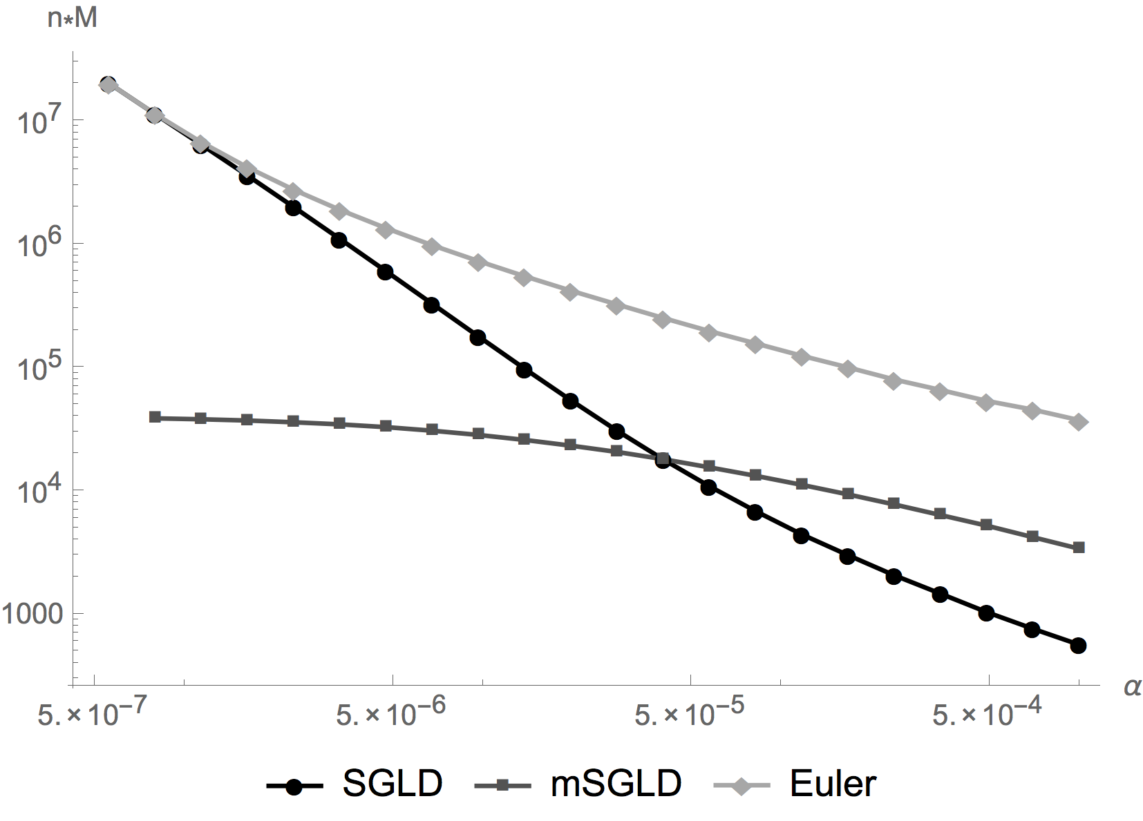
In Section 2.2 we compared the Euler method, the SGLD and the mSGLD for the same choice of r=hA.r=\frac{h}{A}. In the following we numerically minimise the computational effort with respect to the condition MSE2≤ϵ2\text{MSE}_{2}\leq\epsilon^{2}. We assume that the computational cost is proportional to M⋅nM\cdot n which leads to the problem of solving

minF\displaystyle\min_{F} M⋅n\displaystyle M\cdot n (69)
subject to MSE2​(r,M,n)≤ϵ2\displaystyle\text{MSE}_{2}(r,M,n)\leq\epsilon^{2}
w.r.t. r<1,M,n.\displaystyle r<1,M,n.

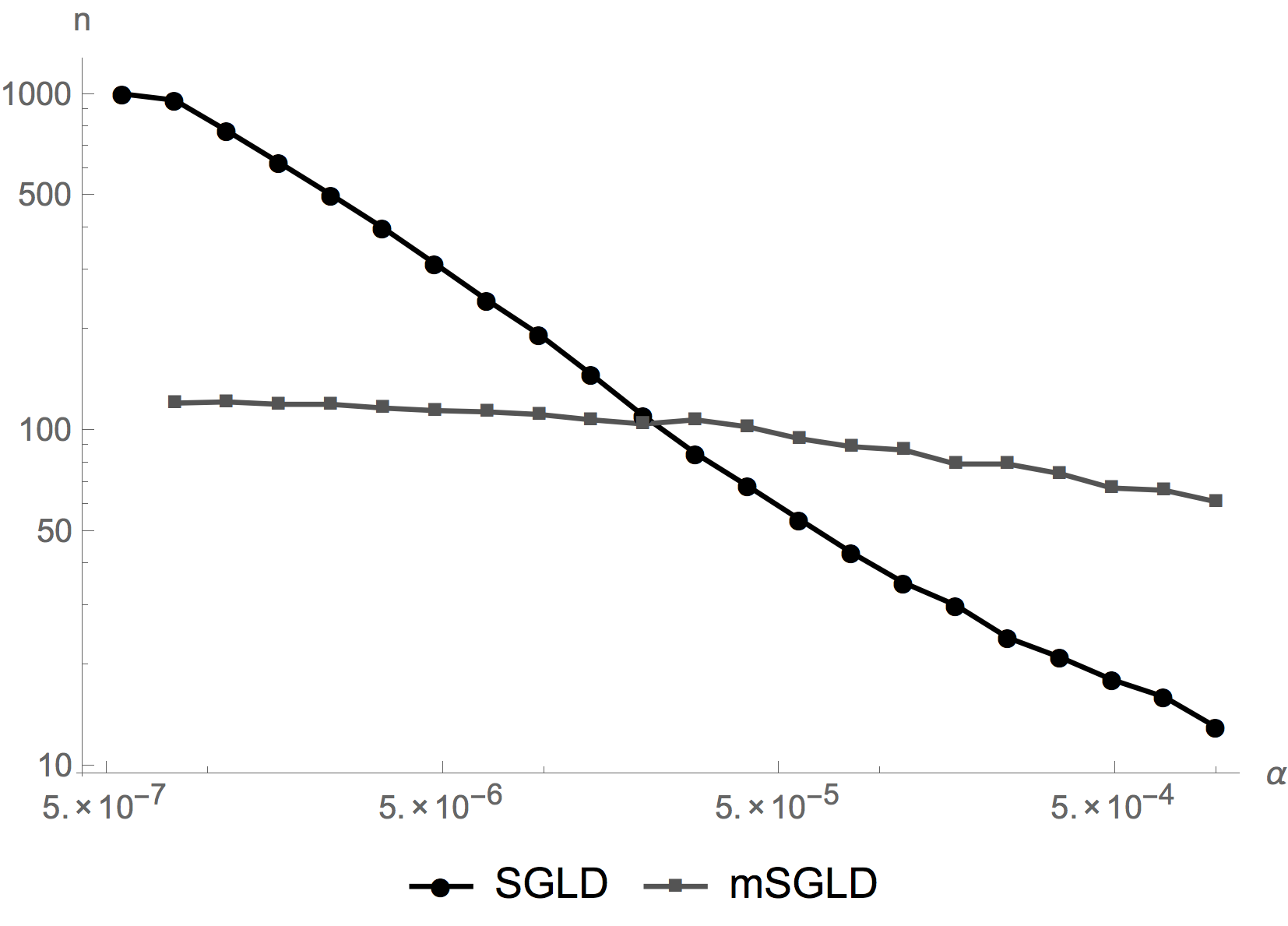
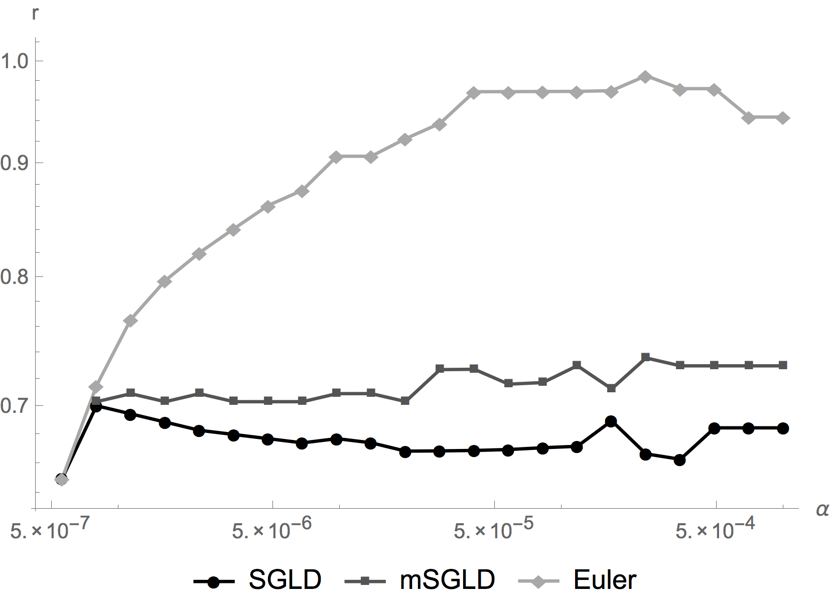
Even though we have analytic expressions for the MSE2\text{MSE}_{2}, the solution to the optimisation problem does not have a closed form. To conclude our analysis, we illustrate the numerical solution to this problem for N=1000N=1000 for the Euler method, the SGLD and the mSGLD. The results, depicted in Figure 3, can be summarised as follows:

  1. 1.

    as ϵ\epsilon becomes smaller, the gain of the SGLD over the Euler method in terms of computational effort decreases (due to the fact that nn increases);

  2. 2.

    as ϵ\epsilon becomes smaller, the mSGLD gains efficiency over the SGLD (the reason being that nn seems to asymptote as ϵ\epsilon decreases).

Refer to caption
(a) Minimised computational cost for the Euler, the SGLD and the mSGLD algorithm
Refer to caption
(b) Subset size nn for minimised computational cost
Refer to caption
(c) Step size r=hAr=\frac{h}{A} for minimised computational cost
Figure 3: Minimisition of computational cost ∝M⋅n\propto M\cdot n subject to M​S​E≤ϵ2MSE\leq\epsilon^{2}

The upper bound obtained in Equation (67) suggests a scaling of M∼ϵ−3M\sim\epsilon^{-3} and r∼ϵr\sim\epsilon to obtain an MSE of order ϵ2\epsilon^{2} with minimal computational effort. The numerical minimisation of MM with respect to rr and MM subject to the condition MSE​(r,M)≤ϵ2\text{MSE}(r,M)\leq\epsilon^{2} confirms this scaling empirically, see Figure 4.

Refer to caption
(a) Line fit yields M⁡(ϵ)∼ϵ−3.03M(\epsilon)\sim\epsilon^{-3.03} as ϵ→0\epsilon\rightarrow 0
Refer to caption
(b) Line fit yields r⁡(ϵ)∼ϵ0.95r(\epsilon)\sim\epsilon^{0.95} as ϵ→0\epsilon\rightarrow 0
Figure 4: Scaling of r⁡(ϵ)r(\epsilon) and M⁡(ϵ)M(\epsilon) for minimal computational cost subject to the MSE2​(r⁡(ϵ),M⁡(ϵ))≤ϵ2\text{MSE}_{2}(r(\epsilon),M(\epsilon))\leq\epsilon^{2}

6.2 The MSE2\text{MSE}_{2} for fixed and increasing NN

We now consider the behaviour for growing data size NN where a new data set XX is generated in each instance. Figure 5 depicts the MSE2\text{MSE}_{2} for N=10iN=10^{i} with i=1,…,4i=1,\dots,4 for the subset choices n=N0.1,N0.5n=N^{0.1},N^{0.5} and N0.9N^{0.9}; each compared to the Euler method corresponding to n=Nn=N. In this plot we notice that the SGLD outperforms the mSGLD for n=N0.1n=N^{0.1} and n=N0.5n=N^{0.5}. The behaviour in Figure 5 suggests that the mSGLD has a larger bias than the SGLD which seems to contradict the findings of Section 2 and 4. Previously, we have just considered the asymptotic of h→0h\rightarrow 0. In contrast, we scale both h=r​1A⁡(N)h=r\frac{1}{A(N)} and n=Npn=N^{p} in terms of NN in Figure 5. In the following we investigate this relationship further by using the explicit formula for the asymptotic bias which has been made available in Section 2 .

For simplicity we consider sampling without replacement, using the expression in Equation (16). Similar conclusions hold for sampling with replacement. First we consider the mSGLD. From Equation (21) and using the parameterisation h=r/Ah=r/A of the step size, the excess asymptotic bias becomes

h2​Var​(B)24​(2​A−A2​h)=(r/A)2​(N−nn)2​N2​Var⁡(X)24​(2−r)​A.h^{2}\frac{\text{Var}(B)^{2}}{4(2A-A^{2}h)}=\frac{(r/A)^{2}\left(\frac{N-n}{n}\right)^{2}N^{2}\Var(X)^{2}}{4(2-r)A}.

Because A∼NA\sim N, we see that the excess bias stays bounded for large NN if and only if n≳N12n\gtrsim N^{\frac{1}{2}}. In contrast, the same consideration for the SGLD shows that the excess bias due to subsampling vanishes so long as n→∞n\rightarrow\infty when N→∞N\rightarrow\infty.

Refer to caption
(a) The SGLD for n=N110n=N^{\frac{1}{10}}
Refer to caption
(b) The mSGLD for n=N110n=N^{\frac{1}{10}}
Refer to caption
(c) The SGLD for n=N12n=N^{\frac{1}{2}}
Refer to caption
(d) The mSGLD for n=N12n=N^{\frac{1}{2}}
Refer to caption
(e) The SGLD for n=N910n=N^{\frac{9}{10}}
Refer to caption
(f) The mSGLD for n=N910n=N^{\frac{9}{10}}
Refer to caption
Figure 5: MSE2\text{MSE}_{2} of the time average for the SGLD and the mSGLD for the second moment of the posterior as N→∞N\rightarrow\infty. Notice that Figures (c) and (d) and (e) and (f) have the same scaling respectively. Moreover, figures (a) and (b) have separate scaling because of the instability of the mSGLD.

We can also identify the regime in which the mSGLD has a smaller asymptotic bias than the SGLD. From Equations (18) and (21) we see that this is the case when

h2​Var2​(B)4​(2​A−A2​h)≤h​Var⁡(B)2​A−A2​h.\frac{h^{2}\operatorname{Var}^{2}(B)}{4(2A-A^{2}h)}\leq\frac{h\operatorname{Var}(B)}{2A-A^{2}h}. (70)

Using Equation (16), the above can be rearranged to

1≥h4​116​σx2​N⁡(N−n)N​Var​(X).1\geq\frac{h}{4}\frac{1}{16\sigma^{2}_{x}}\frac{N(N-n)}{N}\text{Var}(X).

Let c=nNc=\frac{n}{N} be the relative size of the subsampling. Using h=r/Ah=r/A where AA is given in Equation (15), we get

c≥2​r​N​Var​X16​σx2​(1σθ2+Nσx2)+2​r​N​Var​Xc\geq\frac{2rN\text{Var}\,X}{16\sigma^{2}_{x}\left(\frac{1}{\sigma^{2}_{\theta}}+\frac{N}{\sigma^{2}_{x}}\right)+2rN\text{Var}\,X}

which in the limit of large data sets N→∞N\rightarrow\infty yields

c≥2​r​Var​X16+2​r​Var​X>0.c\geq\frac{2r\text{Var}\,X}{16+2r\text{Var}\,X}>0.

In conclusion, for a fixed step size given by r/Ar/A, the mSGLD has a smaller bias than the SGLD if the above holds. In other words, the subsampling size has to be linear in the size of the data set for a fixed choice of rr.

6.3 Limit of the MSE and ERE for well-specified Data as N→∞N\rightarrow\infty

In order to investigate the limit of N→∞N\rightarrow\infty, we need to specify the behaviour of the data as well. We study this in the well-specified case, in other words, we assume that the data is generated by the model for θ†=1\theta^{\dagger}=1. Previously, we have obtained an analytic expression for the expectation of the MSE2\text{MSE}_{2} with respect to the realisation of the noise driving the algorithm. In contrast, we take expectations with respect to the realisation of the data XX and the noise driving the algorithm in the following results. These results are formulated in analytic expressions22 2 see Appendix 10.2 for a sketch of the derivation for the MSE2\text{MSE}_{2} (the derivation for ERE is similar) for the MSE2\text{MSE}_{2} and the ERE depending only on M,n,rM,n,r and NN. We then choose M,nM,n and rr as functions of NN and study the limit N→∞N\rightarrow\infty and how this affects the computational cost and the behaviour of the ERE and the MSE2\text{MSE}_{2} as N→∞N\rightarrow\infty for the different algorithms.

For the Euler method (n=Nn=N) we need to take h<1A≍1Nh<\frac{1}{A}\asymp\frac{1}{N} in order to make Equation (17) stable. Moreover, we need the number of steps MM to be of order NN to approximate the diffusion to a time of order 𝒪⁡(1)\mathcal{O}(1). Because we evaluate NN data points per step, this heuristic argument suggests that the complexity is of order 𝒪⁡(N2)\mathcal{O}\left(N^{2}\right). Furthermore, we verify (using Mathematica®), that for the Euler method (n=Nn=N)

limN→∞𝔼X​MSE=0,limN→∞𝔼X​ERE=0\lim_{N\rightarrow\infty}\mathbb{E}_{X}\text{MSE}=0,\quad\lim_{N\rightarrow\infty}\mathbb{E}_{X}\text{ERE}=0 (71)

for the choices M=N1+2​ϵM=N^{1+2\epsilon} and r=N−ϵr=N^{-\epsilon} for any ϵ>0\epsilon>0. The computational cost for fixed NN is M⋅n=N2+2​ϵM\cdot n=N^{2+2\epsilon}. Thus, this confirms the heuristics we used for the Euler method in Section 6.2.

A natural next question to ask in terms of the SGLD is if one can have Equation (71) to hold but for smaller computational complexity than the Euler method. Using Mathematica®, we obtain the following theorem for the MSE

Theorem 6.1.

For any ϵ>0\epsilon>0 and the choices h=N−1−ϵh=N^{-1-\epsilon}, M=N1+2​ϵM=N^{1+2\epsilon} and n=1,n=1, the SGLD satisfies

limN→∞𝔼θii,X​(1M​∑k=0M−1θj2−(μp2+σp2))2=0.\lim_{N\rightarrow\infty}\mathbb{E}_{{\theta_{i}}_{i},X}\left(\frac{1}{M}\sum_{k=0}^{M-1}\theta_{j}^{2}-(\mu_{p}^{2}+\sigma_{p}^{2})\right)^{2}=0.

This constitutes a substantial gain compared to the Euler method because it reduces the computational complexity in the data size NN from being almost quadratic to almost linear.

We now draw our attention to the expected relative error in estimating the posterior variance, abbreviated by

ERE:=𝔼{θi}i​1K​∑i=0K−1θi2−(1K​∑i=0K−1θi)2σp2−1.\text{ERE}:=\mathbb{E}_{\{\theta_{i}\}_{i}}\frac{\frac{1}{K}\sum_{i=0}^{K-1}\theta_{i}^{2}-\left(\frac{1}{K}\sum_{i=0}^{K-1}\theta_{i}\right)^{2}}{\sigma_{p}^{2}}-1. (72)

Because the posterior variance goes to zero as N⇒∞N\Rightarrow\infty, it is conceivable that it requires more computational effort to ensure that limN→∞𝔼X​ERE=0\lim_{N\rightarrow\infty}\mathbb{E}_{X}\text{ERE}=0. In order to illustrate the behaviour of the ERE, we first consider the behaviour for a fixed data set and repeat the experiment of Figure 5 in Figure 6. The latter demonstrates that the asymptotic bias for the choice n=N12n=N^{\frac{1}{2}} (the asymptotes for the grey lines) have an increasing value in NN. We used h=120​A∼1Nh=\frac{1}{20A}\sim\frac{1}{N} which decreases with NN. However, we show below that is requirement cancels exactly the gain from n≪Nn\ll N at least on the algebraic scale in NN.

Refer to caption
Refer to caption
Figure 6: Expected relative error of the estimate of the variance of the posterior based on the SGLD.

In particular, we now choose r=N−αr=N^{-\alpha}, n=Nβn=N^{\beta} and M=NγM=N^{\gamma}. Hence the computational cost is Nβ+γN^{\beta+\gamma}. The step size h=rAh=\frac{r}{A} satisfies h∼N−1−αh\sim N^{-1-\alpha} because A∼NA\sim N. Since the algorithm performs M=NγM=N^{\gamma} steps, we expect it to approximate the diffusion on the time interval h⋅M=N−1−α+γh\cdot M=N^{-1-\alpha+\gamma}. Therefore it is reasonable to require that γ>1+α\gamma>1+\alpha. Under this assumption and with the help of Mathematica®, we reduced the limit above to

limN→∞𝔼X​ERE\displaystyle\lim_{N\rightarrow\infty}\mathbb{E}_{X}\text{ERE} =limN→∞(2⋅N−α−β+3(N+1)2​(N−α−2)2−N−2​α−β+3(N+1)2​(N−α−2)2)\displaystyle=\lim_{N\rightarrow\infty}\left(\frac{2\cdot N^{-\alpha-\beta+3}}{(N+1)^{2}\left(N^{-\alpha}-2\right)^{2}}-\frac{N^{-2\alpha-\beta+3}}{(N+1)^{2}\left(N^{-\alpha}-2\right)^{2}}\right)
={0if ​α+β>1∞if ​α+β<1.\displaystyle=\begin{cases}0&\text{if }\alpha+\beta>1\\ \infty&\text{if }\alpha+\beta<1.\end{cases}

Thus for limN→∞𝔼X​ERE=0\lim_{N\rightarrow\infty}\mathbb{E}_{X}\text{ERE}=0 it is necessary that α+β≥1\alpha+\beta\geq 1. This condition in turn implies that the computational complexity satisfies

Nγ⏟steps×Nβ⏟cost per step=N1+α​Nβ=N1+α+β≳N2.\underbrace{N^{\gamma}}_{\text{steps}}\times\underbrace{N^{\beta}}_{\text{cost per step}}=N^{1+\alpha}N^{\beta}=N^{1+\alpha+\beta}\gtrsim N^{2}.

Thus, there is no computational gain for the ERE in the limit N→∞N\rightarrow\infty on the algebraic scale in N.N. We note that picking θ⋆=1N\theta^{\star}=\frac{1}{N} instead of θ⋆=1\theta^{\star}=1 does not change the results. Thus, a closer initialisation does not change the result for the ERE.

7 Logistic Regression

In the following we present numerical simulations for a Bayesian logistic regression model. The data items are given by covariates xi∈ℝdx_{i}\in\mathbb{R}^{d} that are labeled by yi∈{−1,1}y_{i}\in\{-1,1\}.We assume the data yi∈{−1,1}y_{i}\in\{-1,1\} is modelled by

p⁡(yi|xi,β)=σ⁡(yi​βt​xi)p(y_{i}|x_{i},\beta)=\sigma(y_{i}\beta^{t}x_{i}) (73)

where σ⁡(z)=11+exp⁡(−z)∈[0,1]\sigma(z)=\frac{1}{1+\exp(-z)}\in[0,1]. The model posses the assumption that yiy_{i} depends on xix_{i} through the linear relationship βt​xi\beta^{t}x_{i}. Nevertheless, logistic regression is commonly used after a preprocessing has taken place and is therefore used here for numerical illustration.

We put a Gaussian prior 𝒩⁡(0,C0)\mathcal{N}(0,C_{0}) on β\beta, for simplicity we use C0=IC_{0}=I subsequently. By Bayes’ rule the posterior π\pi satisfies

π⁡(β)∝exp⁡(−12​‖β‖C02)​∏i=1Nσ⁡(yi​βT​xi).\pi(\beta)\propto\exp\left(-\frac{1}{2}\left\|\beta\right\|_{C_{0}}^{2}\right)\prod_{i=1}^{N}\sigma(y_{i}\beta^{T}x_{i}).

We consider d=3d=3 and N=1000N=1000 data points and choose the covariate to be

x=(x1,1x1,21x2,1x2,21⋮⋮⋮x1000,1x1000,21)x=\left(\begin{array}[]{ccc}x_{1,1}&x_{1,2}&1\\ x_{2,1}&x_{2,2}&1\\ \vdots&\vdots&\vdots\\ x_{1000,1}&x_{1000,2}&1\end{array}\right)

for a fixed sample of xi,j​∼i.i.d.​𝒩​(0,1)x_{i,j}\overset{\text{i.i.d.}}{\sim}\mathcal{N}\left(0,1\right) for i=1,…​1000i=1,\dots 1000 and j=1,2j=1,2. We use a long run of the Random-Walk-Metropolis algorithm to estimate the posterior mean.

On that basis we estimate the MSE of the SGLD based mean estimate using 100100 runs of the algorithm with step size h=0.002h=0.002 for various subset sizes. Figure 7 depicts the MSE as function of the iterations and effective iterations through the data set. Notice that for this example the variance of the stochastic gradient f^​(θ){\hat{f}(\theta)} depends on both θ\theta and all the data items. For this reason we replace Var ​f^​(θ){\text{Var }\hat{f}(\theta)} by an estimate Var ^​f^​(θ){\widehat{\text{Var }}\hat{f}(\theta)}, see also Remark 4.2. We note that the mSGLD is superior for n=150n=150, inferior for n=50n=50 and for n=10n=10 the MSE of the mSGLD does not drop below 11.

Refer to caption
Refer to caption
Figure 7: Expected MSE of time average for the SGLD and the mSGLD for the mean of the posterior

8 Conclusion

This article presents the mathematical foundations that are necessary for posterior sampling for stochastic gradient methods with fixed step sizes. We derived an error expansion of the asymptotic bias in terms of powers of the step size and identified how the constant in the leading order term depends on the unbiased estimator of the gradient. We construct a modified SGLD to match the Euler method in this asymptotic expansion. These asymptotic results are complemented by upper bounds on the bias and the MSE over a finite time horizon. Minimising the MSE with respect to the step size yields a decay of the error at the same rate as the decreasing step size SGLD, see Remark 5.1. These theoretical findings are completed with extensive analytic investigations of a one dimensional toy model that allows the derivation of analytic expressions for the sample average and its moments. Finally, this yields an exact quantification of expected errors. The results of this investigation can be summarised as follows:

  • •

    In the high accuracy regime the SGLD deteriorates to the Euler method while the mSGLD prevails.

  • •

    For small data batches the bias of the mSGLD is larger than for the SGLD.

  • •

    In the limit as the number of data items goes to infinity the SGLD reduces computational complexity of estimating the second moment with vanishing MSE by one power of the number of data items.

This recommends the construction of new and a study of existing modifications of the SGLD such as the Stochastic Gradient Hamiltonian Monte Carlo [Chen et al., 2014] and the Stochastic Gradient Thermostat Monte Carlo [Ding et al., 2014] algorithms.

Acknowledgement

SJV and YWT acknowledge EPSRC for research funding through grant EP/K009850/1 and EP/K009362/1. The authors thank Rémi Bardenet for fruitful discussions.

References

  • [Abdulle et al., 2014] Abdulle, A., Vilmart, G., and Zygalakis, K. (2014). High order numerical approximation of the invariant measure of ergodic sdes. SIAM Journal on Numerical Analysis, 52(4):1600–1622.
  • [Bou-Rabee and Vanden-Eijnden, 2010] Bou-Rabee, N. and Vanden-Eijnden, E. (2010). Pathwise accuracy and ergodicity of metropolized integrators for SDEs. Communications on Pure and Applied Mathematics, 63(5):655–696.
  • [Brooks et al., 2011a] Brooks, S., Gelman, A., Jones, G., and Meng, X. (2011a). Handbook of Markov Chain Monte Carlo. Chapman & Hall/CRC Handbooks of Modern Statistical Methods. CRC Press.
  • [Brooks et al., 2011b] Brooks, S., Gelman, A., Jones, G., and Meng, X.-L. (2011b). Handbook of Markov Chain Monte Carlo. Chapman and Hall/CRC.
  • [Chen et al., 2014] Chen, T., Fox, E., and Guestrin, C. (2014). Stochastic Gradient Hamiltonian Monte Carlo. arXiv Prepr. arXiv1402.4102, pages 1–23.
  • [Debussche and Faou, 2012] Debussche, A. and Faou, E. (2012). Weak backward error analysis for SDEs. SIAM J. Numer. Anal., 50(3):1735–1752.
  • [Ding et al., 2014] Ding, N., Fang, Y., Babbush, R., Chen, C., Skeel, R., and Neven, H. (2014). Bayesian sampling using stochastic gradient thermostats. To Appear in Advances in Neural Information Processing Systems (NIPS), Montreal, Canada.
  • [Hasminskii, 1980] Hasminskii, R. (1980). Stochastic stability of differential equations. Sijthoff and Noordhoff, The Netherlands.
  • [Kopec, 2014] Kopec, M. (2014). Weak backward error analysis for overdamped langevin processes. IMA Journal of Numerical Analysis.
  • [Kopec, 2015] Kopec, M. (2015). Weak backward error analysis for langevin process. BIT Numerical Mathematics, pages 1–47.
  • [Lamberton and Pages, 2002] Lamberton, D. and Pages, G. (2002). Recursive computation of the invariant distribution of a diffusion. Bernoulli, 8(3):367–405.
  • [Leimkuhler and Matthews, 2013] Leimkuhler, B. and Matthews, C. (2013). Rational construction of stochastic numerical methods for molecular sampling. Applied Mathematics Research eXpress, 2013(1):34–56.
  • [Mattingly et al., 2010] Mattingly, J. C., Stuart, A. M., and Tretyakov, M. V. (2010). Convergence of Numerical Time-Averaging and Stationary Measures via Poisson Equations. SIAM J. Numer. Anal., 48(2):552–577.
  • [Milstein, 1986] Milstein, G. (1986). Weak approximation of solutions of systems of stochastic differential equations. Theory Probab. Appl., 30(4):750–766.
  • [Milstein and Tretyakov, 2004] Milstein, G. and Tretyakov, M. (2004). Stochastic numerics for mathematical physics. Scientific Computing. Springer-Verlag, Berlin and New York.
  • [Milstein and Tretyakov, 2007] Milstein, G. N. and Tretyakov, M. V. (2007). Computing ergodic limits for Langevin equations. Phys. D, 229(1):81–95.
  • [Neal, 2011] Neal, R. M. (2011). Markov chain monte carlo using hamiltonian dynamics. In Handbook of Markov Chain Monte Carlo. Chapman & Hall/CRC.
  • [Pardoux and Veretennikov, 2001] Pardoux, E. and Veretennikov, A. Y. (2001). On the Poisson equation and diffusion approximation. I. Ann. Probab., 29(3):1061–1085.
  • [Patterson and Teh, 2013] Patterson, S. and Teh, Y. W. (2013). Stochastic gradient Riemannian Langevin dynamics on the probability simplex. In Advances in Neural Information Processing Systems.
  • [Roberts and Tweedie, 1996] Roberts, G. O. and Tweedie, R. L. (1996). Exponential convergence of Langevin distributions and their discrete approximations. Bernoulli, 2(4):pp. 341–363.
  • [S. Ahn and Welling, 2012] S. Ahn, A. K. and Welling, M. (2012). Bayesian posterior sampling via stochastic gradient fisher scoring. In ICML.
  • [Sato and Nakagawa, 2014] Sato, I. and Nakagawa, H. (2014). Approximation analysis of stochastic gradient langevin dynamics by using fokker-planck equation and ito process. In Jebara, T. and Xing, E. P., editors, Proceedings of the 31st International Conference on Machine Learning (ICML-14), pages 982–990. JMLR Workshop and Conference Proceedings.
  • [Talay and Tubaro, 1990] Talay, D. and Tubaro, L. (1990). Expansion of the global error for numerical schemes solving stochastic differential equations. Stochastic Anal. Appl., 8(4):483–509 (1991).
  • [Teh et al., 2014] Teh, Y. W., Thiéry, A. H., and Vollmer, S. J. (2014). Consistency and fluctuations for stochastic gradient Langevin dynamics. ArXiv e-prints. Accepted by J. Mach. Learn. Res.
  • [Welling and Teh, 2011] Welling, M. and Teh, Y. W. (2011). Bayesian Learning via Stochastic Gradient Langevin Dynamics. In Proceedings of the 28th International Conference on Machine Learning (ICML), pages 681–688.
  • [Zygalakis, 2011] Zygalakis, K. C. (2011). On the existence and applications of modified equations for stochastic differential equations. SIAM J. Sci. Comput., 33:102–130.

9 Appendix A: Finite time Ergodic Average based Poisson Equation

Proof of Theorem 5.2.

Rearranging Equation (61) for 1K​∑k=0K−1(ϕk−ϕ¯)\frac{1}{K}\sum_{k=0}^{K-1}(\phi_{k}-\bar{\phi}), the bias and the MSE can be controlled as follows:

𝔼​1K​h​(ψK−ψ0)≲1T​supi𝔼​Vipψ,0≲1T.\mathbb{E}\frac{1}{Kh}\left(\psi_{K}-\psi_{0}\right)\lesssim\frac{1}{T}\sup_{i}\mathbb{E}V_{i}^{p_{\psi,0}}\lesssim\frac{1}{T}.

Because A0=ℒA_{0}=\mathcal{L} for the SGLD it is left to bound to bound 𝔼​1T​Si,K\mathbb{E}\frac{1}{T}S_{i,K} for i=0​…​4i=0\dots 4. First we consider i=1i=1 and use Equation (A.6)

1T​𝔼​S1,K\displaystyle\frac{1}{T}\mathbb{E}S_{1,K} ≲\displaystyle\lesssim 1T​𝔼​∑k=0K−1h2​Vkpψ,2​𝔼τk​‖f^k‖2\displaystyle\frac{1}{T}\mathbb{E}\sum_{k=0}^{K-1}h^{2}V_{k}^{p_{\psi,2}}\mathbb{E}_{\tau_{k}}\left\|\hat{f}_{k}\right\|^{2}
≲\displaystyle\lesssim 1T​∑k=0K−1h2​supi𝔼​Vipψ,2+1≲1T​h2​K≲h.\displaystyle\frac{1}{T}\sum_{k=0}^{K-1}h^{2}\sup_{i}\mathbb{E}V_{i}^{p_{\psi,2}+1}\lesssim\frac{1}{T}h^{2}K\lesssim h.

This procedure will be used over and over again. It can be summarised as follows:

  1. 1.

    bounding the terms in the sum by a power of VpV^{p}, using Equation (A.6) and the assumption on derivates of ψ\psi;

  2. 2.

    then derive the bound using supi𝔼​Vip<∞\sup_{i}\mathbb{E}V_{i}^{p}<\infty.

For i=2i=2 we additionally use that Equation (65) implies

∫01s3​ψ(4)​(s​θk+(1−s)​θk+1)​(Δk+1,Δk+1,Δk+1,Δk+1)​𝑑s≲(Vkpψ,4+Vk+1pψ,4)​‖Δk‖4.\int_{0}^{1}s^{3}{\psi}^{(4)}\left(s\theta_{k}+(1-s)\theta_{k+1}\right)\left(\Delta_{k+1},\Delta_{k+1},\Delta_{k+1},\Delta_{k+1}\right)ds\lesssim\left(V_{k}^{p_{\psi,4}}+V_{k+1}^{p_{\psi,4}}\right)\left\|\Delta_{k}\right\|^{4}.

which allows us to follow the general procedure

1T​𝔼​S2,K\displaystyle\frac{1}{T}\mathbb{E}S_{2,K} ≲\displaystyle\lesssim 1T​𝔼​∑k=0K−1Rk+1\displaystyle\frac{1}{T}\mathbb{E}\sum_{k=0}^{K-1}R_{k+1}
≲\displaystyle\lesssim 1T​𝔼​∑k=0K−1h2​(Vkpψ,4+Vk+1pψ,4)​𝔼τ​‖Δk+1‖4\displaystyle\frac{1}{T}\mathbb{E}\sum_{k=0}^{K-1}h^{2}\left(V_{k}^{p_{\psi,4}}+V_{k+1}^{p_{\psi,4}}\right)\mathbb{E}_{\tau}\left\|\Delta_{k+1}\right\|^{4}
≲\displaystyle\lesssim 1T​𝔼​∑k=0K−1h2​supi𝔼​Vpψ,4+2​(θi)≲1T​h2≲h.\displaystyle\frac{1}{T}\mathbb{E}\sum_{k=0}^{K-1}h^{2}\sup_{i}\mathbb{E}V^{p_{\psi,4}+2}(\theta_{i})\lesssim\frac{1}{T}h^{2}\lesssim h.

We apply the general procedure to 𝔼​S0,K\mathbb{E}S_{0,K}

1T​𝔼​S0,K\displaystyle\frac{1}{T}\mathbb{E}S_{0,K} ≲\displaystyle\lesssim 1T​𝔼​∑k=0K−1h2​Vkpψ,3​𝔼τ​‖gk​ηk+1‖2​‖f^k‖\displaystyle\frac{1}{T}\mathbb{E}\sum_{k=0}^{K-1}h^{2}V_{k}^{p_{\psi,3}}\mathbb{E}_{\tau}\left\|g_{k}\eta_{k+1}\right\|^{2}\left\|\hat{f}_{k}\right\|
≲\displaystyle\lesssim 1T​𝔼​∑k=0K−1h2​supi𝔼​Vpψ,3+12​(θi)\displaystyle\frac{1}{T}\mathbb{E}\sum_{k=0}^{K-1}h^{2}\sup_{i}\mathbb{E}V^{p_{\psi,3}+\frac{1}{2}}(\theta_{i})
≲\displaystyle\lesssim 1T​h2≲h.\displaystyle\frac{1}{T}h^{2}\lesssim h.
1T​𝔼​S~0,K\displaystyle\frac{1}{T}\mathbb{E}\tilde{S}_{0,K} ≲\displaystyle\lesssim 1T​𝔼​∑k=0K−1h3​Vkpψ,3​𝔼τ​‖f^k‖3\displaystyle\frac{1}{T}\mathbb{E}\sum_{k=0}^{K-1}h^{3}V_{k}^{p_{\psi,3}}\mathbb{E}_{\tau}\left\|\hat{f}_{k}\right\|^{3}
≲\displaystyle\lesssim 1T​∑k=0K−1h3​supi𝔼​Vpψ,3+32​(θl)≲1T​K​h3≲h2.\displaystyle\frac{1}{T}\sum_{k=0}^{K-1}h^{3}\sup_{i}\mathbb{E}V^{p_{\psi,3}+\frac{3}{2}}(\theta_{l})\lesssim\frac{1}{T}Kh^{3}\lesssim h^{2}.

Thus, we have established the bound on the bias given by Equation (9.1).

In order to establish the bound one the MSE in Equation (67) we note that Equation (61) yields

𝔼​(1K​∑k=0K−1(ϕ−ϕ¯))2\displaystyle\mathbb{E}\left(\frac{1}{K}\sum_{k=0}^{K-1}\left(\phi-\bar{\phi}\right)\right)^{2} ≲\displaystyle\lesssim 𝔼​(ψK−ψ)2T2\displaystyle\mathbb{E}\frac{\left(\psi_{K}-\psi\right)^{2}}{T^{2}}
+1T2∑i=02𝔼Si,K2+1T2∑i=02𝔼Mi,K2\displaystyle+\frac{1}{T^{2}}\sum_{i=0}^{2}\mathbb{E}S_{i,K}^{2}+\frac{1}{T^{2}}\sum_{i=0}^{2}\mathbb{E}M_{i,K}^{2}

First we note that

𝔼​(ψK−ψ)2T2≲1T2​supi𝔼​Vi2​pψ,0≲1T2.\mathbb{E}\frac{\left(\psi_{K}-\psi\right)^{2}}{T^{2}}\lesssim\frac{1}{T^{2}}\sup_{i}\mathbb{E}V_{i}^{2p_{\psi,0}}\lesssim\frac{1}{T^{2}}.

The Si,K2S_{i,K}^{2} terms can be bound in similar way as above with the additional use of Cauchy-Schwartz inequality to break the correlation between VipV_{i}^{p} and VjpV_{j}^{p}.

1T2​𝔼​S1,K2\displaystyle\frac{1}{T^{2}}\mathbb{E}S_{1,K}^{2} ≲\displaystyle\lesssim 1T2​𝔼​∑i,j=0K−1h4​∇2ψi​[f^i,f^i]​∇2ψj​[f^j,f^j]\displaystyle\frac{1}{T^{2}}\mathbb{E}\sum_{i,j=0}^{K-1}h^{4}\nabla^{2}\psi_{i}\left[\hat{f}_{i},\hat{f}_{i}\right]\nabla^{2}\psi_{j}\left[\hat{f}_{j},\hat{f}_{j}\right]
≲\displaystyle\lesssim 1T2​𝔼​∑i,j=0K−1h4​‖∇2ψi‖​𝔼τ​‖f^i‖2​‖∇2ψj‖​𝔼τ​‖f^j‖2\displaystyle\frac{1}{T^{2}}\mathbb{E}\sum_{i,j=0}^{K-1}h^{4}\left\|\nabla^{2}\psi_{i}\right\|\mathbb{E}_{\tau}\left\|\hat{f}_{i}\right\|^{2}\left\|\nabla^{2}\psi_{j}\right\|\mathbb{E}_{\tau}\left\|\hat{f}_{j}\right\|^{2}
≲\displaystyle\lesssim 1T2​∑i,j=0K−1h4​𝔼​Vipψ,2+1​Vjpψ,2+1\displaystyle\frac{1}{T^{2}}\sum_{i,j=0}^{K-1}h^{4}\mathbb{E}V_{i}^{p_{\psi,2}+1}V_{j}^{p_{\psi,2}+1}
≲\displaystyle\lesssim 1T2​∑i,j=0K−1h4​(𝔼​Vi2​pψ,2+2)12​(𝔼​Vj2​pψ,2+2)12\displaystyle\frac{1}{T^{2}}\sum_{i,j=0}^{K-1}h^{4}\left(\mathbb{E}V_{i}^{2p_{\psi,2}+2}\right)^{\frac{1}{2}}\left(\mathbb{E}V_{j}^{2p_{\psi,2}+2}\right)^{\frac{1}{2}}
≲\displaystyle\lesssim 1T2​∑i,j=0K−1h4​(supi𝔼​Vi2​pψ,2+2)≲K2​h4T2≲h2\displaystyle\frac{1}{T^{2}}\sum_{i,j=0}^{K-1}h^{4}\left(\sup_{i}\mathbb{E}V_{i}^{2p_{\psi,2}+2}\right)\lesssim\frac{K^{2}h^{4}}{T^{2}}\lesssim h^{2}

Similarly, we bound

1T2​𝔼​S2,K2\displaystyle\frac{1}{T^{2}}\mathbb{E}S_{2,K}^{2} ≲\displaystyle\lesssim 1T2​𝔼​∑i,j=0K−1Ri+1​Rj+1\displaystyle\frac{1}{T^{2}}\mathbb{E}\sum_{i,j=0}^{K-1}R_{i+1}R_{j+1}
≲\displaystyle\lesssim 1T2​𝔼​∑i,j=0K−1(Vipψ,4+Vi+1pψ,4)​(Vjpψ,4+Vj+1pψ,4)​𝔼τ​‖Δi+1‖4​𝔼τ​‖Δj+1‖4\displaystyle\frac{1}{T^{2}}\mathbb{E}\sum_{i,j=0}^{K-1}\left(V_{i}^{p_{\psi,4}}+V_{i+1}^{p_{\psi,4}}\right)\left(V_{j}^{p_{\psi,4}}+V_{j+1}^{p_{\psi,4}}\right)\mathbb{E}_{\tau}\left\|\Delta_{i+1}\right\|^{4}\mathbb{E}_{\tau}\left\|\Delta_{j+1}\right\|^{4}
≲\displaystyle\lesssim h4T2​𝔼​∑i,j=0K−1(Vipψ,4+Vi+1pψ,4)​(Vjpψ,4+Vj+1pψ,4)​Vi2​Vj2\displaystyle\frac{h^{4}}{T^{2}}\mathbb{E}\sum_{i,j=0}^{K-1}\left(V_{i}^{p_{\psi,4}}+V_{i+1}^{p_{\psi,4}}\right)\left(V_{j}^{p_{\psi,4}}+V_{j+1}^{p_{\psi,4}}\right)V_{i}^{2}V_{j}^{2}
≲\displaystyle\lesssim h4T2​∑i,j=0K−1(supi𝔼​Vi2​pψ,4+4)≲K2​h4T2≲h2.\displaystyle\frac{h^{4}}{T^{2}}\sum_{i,j=0}^{K-1}\left(\sup_{i}\mathbb{E}V_{i}^{2p_{\psi,4}+4}\right)\lesssim\frac{K^{2}h^{4}}{T^{2}}\lesssim h^{2}.

Similar bounds can also be obtained for 1T2​𝔼​S0,K2\frac{1}{T^{2}}\mathbb{E}S_{0,K}^{2} and 1T2​𝔼​S~0,K2\frac{1}{T^{2}}\mathbb{E}\tilde{S}_{0,K}^{2}

1T2​𝔼​S0,K2\displaystyle\frac{1}{T^{2}}\mathbb{E}S_{0,K}^{2} ≲\displaystyle\lesssim h4T2​∑i,j=0K−1𝔼​Vipψ,3​‖f^i‖​Vjpψ,3​‖f^j‖\displaystyle\frac{h^{4}}{T^{2}}\sum_{i,j=0}^{K-1}\mathbb{E}V_{i}^{p_{\psi,3}}\left\|\hat{f}_{i}\right\|V_{j}^{p_{\psi,3}}\left\|\hat{f}_{j}\right\|
≲\displaystyle\lesssim h4​K2T2​supi𝔼​Vi2​pψ,3+1≲h2\displaystyle\frac{h^{4}K^{2}}{T^{2}}\sup_{i}\mathbb{E}V_{i}^{2p_{\psi,3}+1}\lesssim h^{2}
1T2​𝔼​S~0,K2\displaystyle\frac{1}{T^{2}}\mathbb{E}\tilde{S}_{0,K}^{2} ≲\displaystyle\lesssim h6T2​∑i,j=0K−1𝔼​Vipψ,3​‖f^i‖3​Vjpψ,3​‖f^j‖3\displaystyle\frac{h{}^{6}}{T^{2}}\sum_{i,j=0}^{K-1}\mathbb{E}V_{i}^{p_{\psi,3}}\left\|\hat{f}_{i}\right\|^{3}V_{j}^{p_{\psi,3}}\left\|\hat{f}_{j}\right\|^{3}
≲\displaystyle\lesssim h6​K2T2​supi𝔼​Vi2​pψ,3+2≲h4\displaystyle\frac{h^{6}K^{2}}{T^{2}}\sup_{i}\mathbb{E}V_{i}^{2p_{\psi,3}+2}\lesssim h^{4}

For Martingale terms the cross terms vanish which allows us to obtain the following bounds

1T2​𝔼​M1,K2\displaystyle\frac{1}{T^{2}}\mathbb{E}M_{1,K}^{2} =\displaystyle= 1T2​∑i=0K−1(𝔼​Dl​m2​ψi​(gil,a​ηi+1a​gim,b​ηi+1b−gik,l​gik,m))2\displaystyle\frac{1}{T^{2}}\sum_{i=0}^{K-1}\left(\mathbb{E}D_{lm}^{2}\psi_{i}\left(g_{i}^{l,a}\eta_{i+1}^{a}g_{i}^{m,b}\eta_{i+1}^{b}-g_{i}^{k,l}g_{i}^{k,m}\right)\right)^{2}
≲\displaystyle\lesssim 1T2​∑i=0K−1supi𝔼​Vi2​pψ,2.\displaystyle\frac{1}{T^{2}}\sum_{i=0}^{K-1}\sup_{i}\mathbb{E}V_{i}^{2p_{\psi,2}}.

The following term is the crucial Martingale term as it yields the 𝒪⁡(1T)\mathcal{O}\left(\frac{1}{T}\right) contribution

1T2​𝔼​M2,K2\displaystyle\frac{1}{T^{2}}\mathbb{E}M_{2,K}^{2} ≲\displaystyle\lesssim 1T2​h​∑k=0K−1𝔼​‖∇ψk‖2​‖gk​ξk+1‖2\displaystyle\frac{1}{T^{2}}h\sum_{k=0}^{K-1}\mathbb{E}\left\|\nabla\psi_{k}\right\|^{2}\left\|g_{k}\xi_{k+1}\right\|^{2}
≲\displaystyle\lesssim 1T2​h​∑k=0K−1𝔼​Vk2​pψ,1≲1T.\displaystyle\frac{1}{T^{2}}h\sum_{k=0}^{K-1}\mathbb{E}V_{k}^{2p_{\psi,1}}\lesssim\frac{1}{T}.

Similarly, we estimate

1T2​𝔼​M3,K2\displaystyle\frac{1}{T^{2}}\mathbb{E}M_{3,K}^{2} ≲\displaystyle\lesssim 1T2​h3​∑k=0K−1𝔼​‖∇2ψk‖2​‖f^k‖2​‖gk​ξk+1‖2\displaystyle\frac{1}{T^{2}}h^{3}\sum_{k=0}^{K-1}\mathbb{E}\left\|\nabla^{2}\psi_{k}\right\|^{2}\left\|\hat{f}_{k}\right\|^{2}\left\|g_{k}\xi_{k+1}\right\|^{2}
≲\displaystyle\lesssim 1T2​h3​∑k=0K−1𝔼​Vk2​pψ,2+1≲h2T.\displaystyle\frac{1}{T^{2}}h^{3}\sum_{k=0}^{K-1}\mathbb{E}V_{k}^{2p_{\psi,2}+1}\lesssim\frac{h^{2}}{T}.

The terms 1T2​𝔼​M0,K2\frac{1}{T^{2}}\mathbb{E}M_{0,K}^{2} and 1T2​𝔼​M~0,K2\frac{1}{T^{2}}\mathbb{E}\tilde{M}_{0,K}^{2} can be bounded in the same way

1T2​𝔼​M0,K2\displaystyle\frac{1}{T^{2}}\mathbb{E}M_{0,K}^{2} ≲\displaystyle\lesssim h3T2​∑k=0K−1𝔼​Vk2​pψ,3≲h3​KT2≤h2T\displaystyle\frac{h^{3}}{T^{2}}\sum_{k=0}^{K-1}\mathbb{E}V_{k}^{2p_{\psi,3}}\lesssim\frac{h^{3}K}{T^{2}}\leq\frac{h^{2}}{T}
1T2​𝔼​M~0,K2\displaystyle\frac{1}{T^{2}}\mathbb{E}\tilde{M}_{0,K}^{2} ≲\displaystyle\lesssim h5T2​∑k=0K−1𝔼​Vk2​pψ,3+2≲h5​KT2≤h4T\displaystyle\frac{h^{5}}{T^{2}}\sum_{k=0}^{K-1}\mathbb{E}V_{k}^{2p_{\psi,3}+2}\lesssim\frac{h^{5}K}{T^{2}}\leq\frac{h^{4}}{T}

The additional part for the SGLD is the term corresponding to the Martingale M4,KM_{4,K}

1T2​M4,K2\displaystyle\frac{1}{T^{2}}M_{4,K}^{2} ≲\displaystyle\lesssim 1T2​𝔼​h2​∑k=0K−1(∇ψk​(Hk))2\displaystyle\frac{1}{T^{2}}\mathbb{E}h^{2}\sum_{k=0}^{K-1}\left(\nabla\psi_{k}(H_{k})\right)^{2}
≲\displaystyle\lesssim 1T2​𝔼​h2​∑k=0K−1V2​pψ,1​𝔼τ​‖Hk‖2\displaystyle\frac{1}{T^{2}}\mathbb{E}h^{2}\sum_{k=0}^{K-1}V^{2p_{\psi,1}}\mathbb{E}_{\tau}\left\|H_{k}\right\|^{2}
≲\displaystyle\lesssim 1T2​h2​∑k=0K−1𝔼​V2​pψ,1+1≲hT\displaystyle\frac{1}{T^{2}}h^{2}\sum_{k=0}^{K-1}\mathbb{E}V^{2p_{\psi,1}+1}\lesssim\frac{h}{T}

For all these calculations to go through need supiE​Vip⋆\sup_{i}EV_{i}^{p^{\star}} to be bounded. Collecting the orders present, we see that

p⋆=max⁡{2​pψ,2+2,2​pψ,4+4,2​pψ,3+1,2​pψ,3+3}p^{\star}=\max\left\{2p_{\psi,2}+2,2p_{\psi,4}+4,2p_{\psi,3}+1,2p_{\psi,3}+3\right\}

is sufficient. □\square

9.1 Sufficient Conditions on π\pi Ensuring Finite Time Bounds on Bias and MSE

We formulate a sufficient condition on π\pi that ensure that Theorem 5.2 is applicable. This hinges on deriving a sufficient condition for Equations (62), (64) and (65). The aim of this section is to establish and motivate the sufficient condition formulated in the following theorem.

Theorem 9.1.

Suppose the following condition holds

⟨θ,∇log⁡π0​(θ)⟩\displaystyle\left\langle\theta,\,\,\nabla\log\pi_{0}(\theta)\right\rangle\,\; ≤−α​‖θ‖2+β\displaystyle\leq\,-\alpha\,\left\|\theta\right\|^{2}+\beta (A.1)
⟨θ,∇log⁡π​(Xi∣θ)⟩\displaystyle\left\langle\theta,\,\,\nabla\log\pi(X_{i}\mid\theta)\right\rangle\,\; ≤−α​‖θ‖2+β​ for ​i=1,…,N.\displaystyle\leq\,-\alpha\,\left\|\theta\right\|^{2}+\beta\text{ for }i=1,\dots,N. (A.2)

then Theorem 5.2 is applicable for polynomially bounded and continuous ϕ\phi, that is

Bias​(ϕ^K)\displaystyle\text{Bias}\left(\hat{\phi}_{K}\right) =\displaystyle= |𝔼​ϕ^K−ϕ¯|≤C⁡(h+1K​h)\displaystyle\left|\mathbb{E}\hat{\phi}_{K}-\bar{\phi}\right|\leq C\left(h+\frac{1}{Kh}\right)
𝔼​(ϕ^K−ϕ¯)2\displaystyle\mathbb{E}\left(\hat{\phi}_{K}-\bar{\phi}\right)^{2} ≤\displaystyle\leq C⁡(h2+1K​h)\displaystyle C\left(h^{2}+\frac{1}{Kh}\right)

First we appeal to a sufficient condition for Equation(64) before summarising a regularity results of [Pardoux and Veretennikov, 2001] which allows us to establish Equation (62). We believe that the sufficient conditions above can be weakened, but this requires improving the results of [Pardoux and Veretennikov, 2001] which is out of the scope of this article.

The condition supk𝔼​Vp​(θk)<∞\sup_{k}\mathbb{E}V^{p}\left(\theta_{k}\right)<\infty (that is Equation (64)) is established for all p≤p⋆p\leq p^{\star} by Lemma 5 in [Teh et al., 2014] if p⋆p^{\star} satisfies the following assumption.

Assumption 9.1.

The drift term θ↦12∇logπ(θ)\theta\mapsto\frac{1}{2}\,\nabla\log\pi(\theta) is continuous. The function V:ℝd→[1,∞)V:\mathbb{R}^{d}\to[1,\infty) tends to infinity as ‖θ‖→∞\|\theta\|\to\infty, is twice differentiable with bounded second derivatives and satisfies the following conditions:

  1. 1.

    V is a Lyapunov function for the Langevin dynamics, i.e. there are constants α,β>0\alpha,\beta>0 such that for every θ∈ℝd\theta\in\mathbb{R}^{d} we have

    ⟨∇V(θ),12∇logπ(θ)⟩≤−αV(θ)+β.\,\left\langle\nabla V(\theta),\,\frac{1}{2}\,\nabla\log\pi(\theta)\right\rangle\,\;\leq\,-\alpha\,V(\theta)+\beta. (A.3)
  2. 2.

    The following bounds hold

    • •

      There exists an exponent pH≥2p_{H}\geq 2 such that

      𝔼⁡[‖H⁡(θ,𝒰)‖2​pH]≲VpH​(θ).\mathbb{E}[\,\|H(\theta,\mathcal{U})\|^{2p_{H}}\,]\lesssim V^{p_{H}}(\theta). (A.4)

      Moreover, this implies that 𝔼⁡[‖H⁡(θ,𝒰)‖2​p]≲Vp​(θ)\mathbb{E}[\,\|H(\theta,\mathcal{U})\|^{2p}\,]\lesssim V^{p}(\theta) for any exponent 0≤p≤pH0\leq p\leq p_{H}.

    • •

      For every θ∈ℝd\theta\in\mathbb{R}^{d} we have

      ‖∇V​(θ)‖2+‖∇log⁡π​(θ)‖2≲V⁡(θ).\|\nabla V(\theta)\|^{2}+\|\nabla\log\pi(\theta)\|^{2}\;\lesssim\;V(\theta). (A.5)

Notice that for f^\hat{f} based on subsampling we obtain that pH=∞p_{H}=\infty if

‖∇log⁡p​(y∣θ)‖2≤C⁡(y)​V.\left\|\nabla\log p\left(y\mid\theta\right)\right\|^{2}\leq C(y)V.

Notice that Assumption 9.1 also implies

𝔼​‖θk+1−θk‖2​p\displaystyle\mathbb{E}\left\|\theta_{k+1}-\theta_{k}\right\|^{2p} ≤Vkp\displaystyle\leq V_{k}^{p} (A.6)
𝔼​‖f^k‖2​p\displaystyle\mathbb{E}\left\|\hat{f}_{k}\right\|^{2p} ≤Vkp\displaystyle\leq V_{k}^{p}

if for p≤pHp\leq p_{H}. Equation (65) could now simply be formulated as an additional assumption, however currently we need even stronger assumptions to verify Equation (62). Subsequently, we show how the results of [Pardoux and Veretennikov, 2001] can be used to establish Equation (62) if Equations (A.3) and (A.5) hold for V=‖θ‖2+1V=\left\|\theta\right\|^{2}+1.

Theorem 1 and 2 of [Pardoux and Veretennikov, 2001] characterise the smoothness and growth of the solution to the Poisson equation associated with Equation (60). This is important for our results because the key ingredient for the proof of Theorem 5.2 is

supk𝔼⁡‖ψ((i))​(θk)‖<∞​ for ​k=1,…,4.\sup_{k}\mathbb{E}\left\|{\psi}^{((i))}\left(\theta_{k}\right)\right\|<\infty\text{ for }k=1,\dots,4.

Because we have already established in Section 4 that

supi𝔼​Vp​(θi)<∞\sup_{i}\mathbb{E}V^{p}\left(\theta_{i}\right)<\infty it is left to verify

‖ψ(k)‖\displaystyle\left\|{\psi}^{(k)}\right\| ≲Vpψ,k, for k=0,…,4\displaystyle\lesssim V^{p_{\psi,k}},\quad\text{ for }k=0,\dots,4 (62)
††margin: here

The assumptions needed to apply the Theorem 5.2 results are

⟨f⁡(θ),θ‖θ‖⟩\displaystyle\left\langle f(\theta),\frac{\theta}{\left\|\theta\right\|}\right\rangle ≤\displaystyle\leq −r⁡‖θ‖,‖θ‖≥M0\displaystyle-r\left\|\theta\right\|,\quad\left\|\theta\right\|\geq M_{0} (A.7)
0<λ−\displaystyle 0<\lambda_{-} ≤\displaystyle\leq ⟨g⁡(θ)​g⋆​(θ)​θ‖θ‖,θ‖θ‖⟩≤λ+<∞.\displaystyle\left\langle g\left(\theta\right)g^{\star}\left(\theta\right)\frac{\theta}{\left\|\theta\right\|},\frac{\theta}{\left\|\theta\right\|}\right\rangle\leq\lambda_{+}<\infty. (A.8)

This holds if Assumption 9.1 is satisfied with V⁡(θ)=‖θ‖2+1V\left(\theta\right)=\left\|\theta\right\|^{2}+1.

Theorem 9.2.

[Pardoux and Veretennikov, 2001] Let f¯=0\bar{f}=0 and Equations (A.7) and (A.8) are satisfied. Then there exists a solution ψ∈Wloc2\psi\in W_{\text{loc}}^{2} to the Poisson equation

ℒ​ψ=ϕ−ϕ¯\mathcal{L}\psi=\phi-\bar{\phi}
  1. 1.

    If there is a C such that

    |ϕ⁡(θ)|≤C​(1+‖θ‖)β\left|\phi(\theta)\right|\leq C\left(1+\left\|\theta\right\|\right)^{\beta}

    for some β<0\beta<0, then uu is bounded. Moreover,

    supθ|ψ⁡(θ)|≤C​supθ|f|​(1+‖θ‖)−β\sup_{\theta}\left|\psi(\theta)\right|\leq C\sup_{\theta}\left|f\right|\left(1+\left\|\theta\right\|\right)^{-\beta}

    and

    ‖∇ψ‖≤C\left\|\nabla\psi\right\|\leq C
  2. 2.

    if there exists a constant CC and some β>0\beta>0 such that

    |ϕ⁡(θ)|≤C​(1+‖θ‖)β\left|\phi(\theta)\right|\leq C(1+\left\|\theta\right\|)^{\beta}

    then there exist a constant such that

    |ψ⁡(θ)|≤C′​(1+‖θ‖)β.\left|\psi\left(\theta\right)\right|\leq C^{\prime}\left(1+\left\|\theta\right\|\right)^{\beta}.

    Finally there exists CC such that

    ‖∇ψ‖≤C⁡(1+|θ|β).\left\|\nabla\psi\right\|\leq C\left(1+\left|\theta\right|^{\beta}\right).
Remark 9.3.

We believe that assumption Theorem 9.2 can be weakened to be of the form of Equation (A.3) but it is out of the scope of this article to explore this direction.

In order to iterate Theorem 9.2 we note that the derivatives ψ\psi can be expressed as solution to Poisson equations with different RHSs.

ℒ​ψ\displaystyle\mathcal{L}\psi =\displaystyle= ϕ−ϕ¯\displaystyle\phi-\bar{\phi} (A.9)
A​∂iψ\displaystyle A\partial_{i}\psi =\displaystyle= ∂iϕ−12∇ψ⋅∂if\displaystyle\partial_{i}\phi-\frac{1}{2}\nabla\psi\cdot\partial_{i}f (A.10)
A​∂i​jψ\displaystyle A\partial_{ij}\psi =\displaystyle= ∂i​jϕ−12∇∂jψ⋅∂if−12∇ψ⋅∂i​jf−12∇ψ⋅∂jf\displaystyle\partial_{ij}\phi-\frac{1}{2}\nabla\partial_{j}\psi\cdot\partial_{i}f-\frac{1}{2}\nabla\psi\cdot\partial_{ij}f-\frac{1}{2}\nabla\psi\cdot\partial_{j}f (A.11)
A​∂i​j​kψ\displaystyle A\partial_{ijk}\psi =\displaystyle= ∂i​j​kϕ−12∇∂j​kψ⋅∂if−12∇∂jψ⋅∂i​kf−12∇∂kψ⋅∂i​jf−12∇ψ⋅∂i​j​kf\displaystyle\partial_{ijk}\phi-\frac{1}{2}\nabla\partial_{jk}\psi\cdot\partial_{i}f-\frac{1}{2}\nabla\partial_{j}\psi\cdot\partial_{ik}f-\frac{1}{2}\nabla\partial_{k}\psi\cdot\partial_{ij}f-\frac{1}{2}\nabla\psi\cdot\partial_{ijk}f (A.12)
−12∇∂kψ⋅∂j​kf−12∇ψ⋅∂j​kf−12∇ψ⋅∂kf\displaystyle-\frac{1}{2}\nabla\partial_{k}\psi\cdot\partial_{jk}f-\frac{1}{2}\nabla\psi\cdot\partial_{jk}f-\frac{1}{2}\nabla\psi\cdot\partial_{k}f

We will denote by βψ,i\beta_{\psi,i} numbers that satisfy

sup|α|=i‖∂αψ‖≲(1+|θ|βψ,i)\sup_{\left|\alpha\right|=i}\left\|\partial^{\alpha}\psi\right\|\lesssim\left(1+\left|\theta\right|^{\beta_{\psi,i}}\right) (A.13)

where we used multi-index notation for derivatives. We use a similar notation for the derivatives of ff, that is βf,i\beta_{f,i} and assume that these bounds are a priori given.

Using Theorem 9.2 we can obtain pψ,ip_{\psi,i} to satisfy Equation (62) in terms of the β\beta’s which we formulate as the following lemma.

Lemma 9.4.

Suppose that ϕ\phi and its derivatives are bounded and Assumption 9.1 and Equations Equations (A.7) and (A.8) hold. Then the choice

pψ,0\displaystyle p_{\psi,0} =\displaystyle= 0\displaystyle 0
pψ,1\displaystyle p_{\psi,1} =\displaystyle= 0\displaystyle 0
pψ,2\displaystyle p_{\psi,2} =\displaystyle= βf,12\displaystyle\frac{\beta_{f,1}}{2}
pψ,3\displaystyle p_{\psi,3} =\displaystyle= βf,1∨βf,22\displaystyle\beta_{f,1}\vee\frac{\beta_{f,2}}{2}
pψ,4\displaystyle p_{\psi,4} =\displaystyle= 12(3βf,1∨(βf,1+βf,2.)∨βf,3)\displaystyle\frac{1}{2}\left(3\beta_{f,1}\vee\left(\beta_{f,1}+\beta_{f,2}.\right)\vee\beta_{f,3}\right)

satisfies Equation (62).

Proof.

Assumption 9.1 yields that βf,0=1\beta_{f,0}=1 is a valid choice. Applying Theorem 9.2 to Equation (A.9) implies that βψ,0:=βψ,1:=0\beta_{\psi,0}:=\beta_{\psi,1}:=0 satisfies Equation (A.13). Applying Theorem 9.2 to Equation (A.10) yields that

βψ,2≤βf,1.\beta_{\psi,2}\leq\beta_{f,1}.

Applying Theorem 9.2 to Equation (A.11) yields that

βψ,3≤2​βf,1∨βf,2.\beta_{\psi,3}\leq 2\beta_{f,1}\vee\beta_{f,2}.

Applying Theorem 9.2 to Equation (A.12) yields that

βψ,4\displaystyle\beta_{\psi,4} ≤\displaystyle\leq (βf,1+(2βf,1∨βf,2.))∨(βf,1+βf,2.)∨βf,3\displaystyle\left(\beta_{f,1}+\left(2\beta_{f,1}\vee\beta_{f,2}.\right)\right)\vee\left(\beta_{f,1}+\beta_{f,2}.\right)\vee\beta_{f,3}
≤\displaystyle\leq 3βf,1∨(βf,1+βf,2.)∨βf,3.\displaystyle 3\beta_{f,1}\vee\left(\beta_{f,1}+\beta_{f,2}.\right)\vee\beta_{f,3}.

Thus we have established Equation (62). □\square

10 Analytic expressions for the Gaussian Toy Model

We sketch the derivation of the analytic expression of the MSE are used for the plots in Section 6.

10.1 Expected MSE for fixed Data Sets

We outline how an analytic expression for the MSE of the sample average can be derived. The following method generalises to any polynomial test function but we concentrate on the sample average for the second moment of the posterior given by S2=1M​∑j=0M−1θj2.S_{2}=\frac{1}{M}\sum_{j=0}^{M-1}\theta_{j}^{2}. Its MSE can be expressed using Equation (12)

M​S​E=𝔼​(1M​∑k=0M−1θj2−(μp2+σp2))2=𝔼​S22−2​𝔼​S2​(μp2+σp2)+(μp2+σp2)2.MSE=\mathbb{E}\left(\frac{1}{M}\sum_{k=0}^{M-1}\theta_{j}^{2}-(\mu_{p}^{2}+\sigma_{p}^{2})\right)^{2}=\mathbb{E}S_{2}^{2}-2\mathbb{E}S_{2}\left(\mu_{p}^{2}+\sigma_{p}^{2}\right)+\left(\mu_{p}^{2}+\sigma_{p}^{2}\right)^{2}. (C.1)

In order to express 𝔼​S22\mathbb{E}S_{2}^{2} in Equation (C.1) we derive the recurrence equations for 𝔼​θji\mathbb{E}\theta_{j}^{i} for i=1,…,4i=1,\dots,4 by taking the expectations of

θj+1\displaystyle\theta_{j+1} =(1−A​h)​θj+h​Bj+h​ηj\displaystyle=(1-A\,h)\theta_{j}+hB_{j}+\sqrt{h}\eta_{j}
θj+12\displaystyle\theta_{j+1}^{2} =(1−A​h)2​θj2+h2​Bj2+h​ηj2+2​(1−A​h)​θj​h​Bj+2​(1−A​h)​θj​h​ηj+2​h​Bj​h​ηj\displaystyle=(1-A\,h)^{2}\theta_{j}^{2}+h^{2}B_{j}^{2}+h\eta_{j}^{2}+2(1-A\,h)\theta_{j}hB_{j}+2(1-A\,h)\theta_{j}\sqrt{h}\eta_{j}+2hB_{j}\sqrt{h}\eta_{j} (C.2)
θj+13\displaystyle\theta_{j+1}^{3} =((1−A​h)​θj+h​Bj+h​ηj)3\displaystyle=\left((1-A\,h)\theta_{j}+hB_{j}+\sqrt{h}\eta_{j}\right)^{3}
=(1−A​h)3​θj3+3​(1−A​h)2​θj2​h​Bj+3​(1−A​h)​θj​h2​Bj2+h3​Bj3\displaystyle=(1-A\,h)^{3}\theta_{j}^{3}+3(1-A\,h)^{2}\theta_{j}^{2}hB_{j}+3(1-A\,h)\theta_{j}h^{2}B_{j}^{2}+h^{3}B_{j}^{3}
+3​h​η​(…)+3​η2​h​((1−A​h)​θj+h​Bj)+η3​h32\displaystyle+3\sqrt{h}\eta\left(\dots\right)+3\eta^{2}h\left((1-A\,h)\theta_{j}+hB_{j}\right)+\eta^{3}h^{\frac{3}{2}}
θj+14\displaystyle\theta_{j+1}^{4} =(1−A​h)4​θj4+4​(1−A​h)3​θj3​h​Bj+6​(1−A​h)2​θj2​h2​Bj2\displaystyle=(1-A\,h)^{4}\theta_{j}^{4}+4(1-A\,h)^{3}\theta_{j}^{3}hB_{j}+6(1-A\,h)^{2}\theta_{j}^{2}h^{2}B_{j}^{2} (C.3)
+4​(1−A​h)​θj​h3​Bj3+h4​Bj4+4​η​(…)+4​η3​(…)\displaystyle+4(1-A\,h)\theta_{j}h^{3}B_{j}^{3}+h^{4}B_{j}^{4}+4\eta\left(\dots\right)+4\eta^{3}\left(\dots\right) (C.4)
+6​h​η2​((1−A​h)2​θj2+2​(1−A​h)​θj​h​Bj+h2​Bj2)+η4​h2.\displaystyle+6h\eta^{2}\left((1-A\,h)^{2}\theta_{j}^{2}+2(1-A\,h)\theta_{j}hB_{j}+h^{2}B_{j}^{2}\right)+\eta^{4}h^{2}. (C.5)

The recurrent equation for 𝔼​θj\mathbb{E}\theta_{j} is linear and first order and can therefore be solved explicitly. Plugging the result into the equation for 𝔼​θj2\mathbb{E}\theta_{j}^{2} turns it into a first order linear equation as well. Repeating this processes yields explicit expressions for 𝔼​θji\mathbb{E}\theta_{j}^{i} i=1,…,4i=1,\dots,4.The sums can be carried out explicitly because the terms are of the form of a geometric sum or a geometric term with a polynomial factor. This allows us to obtain an analytic expression for 𝔼​S22\mathbb{E}S_{2}^{2} by reducing it to 𝔼​θji\mathbb{E}\theta_{j}^{i} as follows

𝔼​S22=1M2​𝔼​(∑i=0M−1θi4+2​∑i=0M−1θi2​∑j=i+1M−1θj2).\mathbb{E}S_{2}^{2}=\frac{1}{M^{2}}\mathbb{E}\left(\sum_{i=0}^{M-1}\theta_{i}^{4}+2\sum_{i=0}^{M-1}\theta_{i}^{2}\sum_{j=i+1}^{M-1}\theta_{j}^{2}\right). (C.6)

The cross terms can be removed using Equation (C.2) so that

θj2\displaystyle\theta_{j}^{2} =\displaystyle= (1−A​h)2​(j−i)​θi2+∑k=0j−1−i(1−A​h)2​k\displaystyle\left(1-Ah\right)^{2(j-i)}\theta_{i}^{2}+\sum_{k=0}^{j-1-i}\left(1-Ah\right)^{2k} (C.7)
[h2Bj−1−k2+h2ηj−1−k2+2(1−Ah)Bj−1−khθj−1−k+\displaystyle\left[h^{2}B_{j-1-k}^{2}+h^{2}\eta_{j-1-k}^{2}+2\left(1-Ah\right)B_{j-1-k}h\theta_{j-1-k}+\right.
+2(1−Ah)ηj−1−kθj−1−kh+2h32Bj−1−kηj−1−k].\displaystyle\left.+2\left(1-Ah\right)\eta_{j-1-k}\theta_{j-1-k}\sqrt{h}+2h^{\frac{3}{2}}B_{j-1-k}\eta_{j-1-k}\right].

Plugging this into Equation (C.6) yields

𝔼​S22\displaystyle\mathbb{E}S_{2}^{2} =\displaystyle= 𝔼​1M2​∑i=0M−1θi4​(1+2​∑j=i+1M−1(1−A​h)2​(j−i))\displaystyle\mathbb{E}\frac{1}{M^{2}}\sum_{i=0}^{M-1}\theta_{i}^{4}\left(1+2\sum_{j=i+1}^{M-1}\left(1-Ah\right)^{2(j-i)}\right)
+𝔼1M2∑i=0M−1θi2∑j=i+1M−1∑k=0j−1−i(1−Ah)2​k\displaystyle+\mathbb{E}\frac{1}{M^{2}}\sum_{i=0}^{M-1}\theta_{i}^{2}\sum_{j=i+1}^{M-1}\sum_{k=0}^{j-1-i}\left(1-Ah\right)^{2k}
[h2Bj−1−k2+hηj−1−k2+2(1−Ah)Bj−1−khθj−1−k\displaystyle\quad\left[h^{2}B_{j-1-k}^{2}+h\eta_{j-1-k}^{2}+2\left(1-Ah\right)B_{j-1-k}h\theta_{j-1-k}\right.
+2(1−Ah)ηj−1−kh+2h32Bj−1−kηj−1−k].\displaystyle\quad\left.+2\left(1-Ah\right)\eta_{j-1-k}\sqrt{h}+2h^{\frac{3}{2}}B_{j-1-k}\eta_{j-1-k}\right].

Using the recurrence Equation to express θj−1−k\theta_{j-1-k} in terms of θi\theta_{i} we conclude that 𝔼​S22\mathbb{E}S_{2}^{2} is equal to

1M2​∑i=0M−1𝔼​θi4​(1+2​∑j=i+1M−1(1−A​h)j−i)\displaystyle\frac{1}{M^{2}}\sum_{i=0}^{M-1}\mathbb{E}\theta_{i}^{4}\left(1+2\sum_{j=i+1}^{M-1}\left(1-Ah\right)^{j-i}\right)
+1M2∑i=0M−1𝔼θi2∑j=i+1M−1∑k=0j−1−i(1−Ah)2​k[h2𝔼B2+h].\displaystyle+\frac{1}{M^{2}}\sum_{i=0}^{M-1}\mathbb{E}\theta_{i}^{2}\sum_{j=i+1}^{M-1}\sum_{k=0}^{j-1-i}\left(1-Ah\right)^{2k}\left[h^{2}\mathbb{E}B^{2}+h\right].
+𝔼1M2∑i=0M−1θi2∑j=i+1M−1∑k=0j−1−i(1−Ah)2​k2(1−Ah)Bj−1−kh\displaystyle+\mathbb{E}\frac{1}{M^{2}}\sum_{i=0}^{M-1}\theta_{i}^{2}\sum_{j=i+1}^{M-1}\sum_{k=0}^{j-1-i}\left(1-Ah\right)^{2k}2\left(1-Ah\right)B_{j-1-k}h
((1−A​h)(j−1−k)−i​θi+∑l=0(j−1−k)−i−1(1−A​h)l​(h​Bj−1−k−l−1+h​ηj−1−k−l−1))\displaystyle\left((1-Ah)^{(j-1-k)-i}\theta_{i}+\sum_{l=0}^{(j-1-k)-i-1}(1-Ah)^{l}\left(hB_{j-1-k-l-1}+\sqrt{h}\eta_{j-1-k-l-1}\right)\right)

Taking the expectations into the sum yields

𝔼​S22\displaystyle\mathbb{E}S_{2}^{2} =\displaystyle= 1M2​∑i=0M−1𝔼​θi4​(1+2​∑j=i+1M−1(1−A​h)j−i)\displaystyle\frac{1}{M^{2}}\sum_{i=0}^{M-1}\mathbb{E}\theta_{i}^{4}\left(1+2\sum_{j=i+1}^{M-1}\left(1-Ah\right)^{j-i}\right)
+1M2∑i=0M−1𝔼θi2∑j=i+1M−1∑k=0j−1−i(1−Ah)2​k[h2𝔼B2+h].\displaystyle+\frac{1}{M^{2}}\sum_{i=0}^{M-1}\mathbb{E}\theta_{i}^{2}\sum_{j=i+1}^{M-1}\sum_{k=0}^{j-1-i}\left(1-Ah\right)^{2k}\left[h^{2}\mathbb{E}B^{2}+h\right].
+𝔼1M2∑i=0M−1𝔼θi3∑j=i+1M−1∑k=0j−1−i(1−Ah)2​k2(1−Ah)𝔼Bh(1−Ah)(j−1−k)−i\displaystyle+\mathbb{E}\frac{1}{M^{2}}\sum_{i=0}^{M-1}\mathbb{E}\theta_{i}^{3}\sum_{j=i+1}^{M-1}\sum_{k=0}^{j-1-i}\left(1-Ah\right)^{2k}2\left(1-Ah\right)\mathbb{E}Bh(1-Ah)^{(j-1-k)-i}
+1M2∑i=0M−1𝔼θi2∑j=i+1M−1∑k=0j−1−i(1−Ah)2​k2(1−Ah)𝔼Bh∑l=0(j−1−k)−i−1(1−Ah)lh𝔼B.\displaystyle+\frac{1}{M^{2}}\sum_{i=0}^{M-1}\mathbb{E}\theta_{i}^{2}\sum_{j=i+1}^{M-1}\sum_{k=0}^{j-1-i}\left(1-Ah\right)^{2k}2\left(1-Ah\right)\mathbb{E}Bh\sum_{l=0}^{(j-1-k)-i-1}(1-Ah)^{l}h\mathbb{E}B.

We have an expressions for 𝔼​B\mathbb{E}B but in the following we derive the expressions for 𝔼​B2\mathbb{E}B^{2} required to express 𝔼​S22\mathbb{E}S_{2}^{2}. The terms 𝔼​B3\mathbb{E}B^{3} and 𝔼​B4\mathbb{E}B^{4} are needed for the derivation of 𝔼​θj4\mathbb{E}\theta_{j}^{4}. In order to derive expressions for 𝔼​Bp\mathbb{E}B^{p}, we introduce the power sums

pk=∑i=1NXikp_{k}=\sum_{i=1}^{N}X_{i}^{k}

and the elementary symmetric polynomials

e0=1,e1=∑i=1NXi,e2=∑1≤i<j≤NXiXj,,…,eN=∏i=1NXi.e_{0}=1,e_{1}=\sum_{i=1}^{N}X_{i},e_{2}{\textstyle=\sum_{1\leq i<j\leq N}X_{i}X_{j},},\dots,e_{N}=\prod_{i=1}^{N}X_{i}. (C.8)

Computing eie_{i} naively has complexity of order 𝒪⁡(Ni)\mathcal{O}\left(N^{i}\right) for i≪Ni\ll N. Using Newton’s identities

e1=p1,e2=12​(e1​p1−p2),e3=13​(−e1​p2+e2​p1+p3),e4=14​(e1​p3−e2​p2+e3​p1−p4)e_{1}=p_{1},e_{2}=\frac{1}{2}\left(e_{1}p_{1}-p_{2}\right),e_{3}=\frac{1}{3}\left(-e_{1}p_{2}+e_{2}p_{1}+p_{3}\right),e_{4}=\frac{1}{4}\left(e_{1}p_{3}-e_{2}p_{2}+e_{3}p_{1}-p_{4}\right)

eie_{i} can be expressed in terms of pkp_{k}, k≤ik\leq i each of which can be computed with complexity of order 𝒪⁡(N)\mathcal{O}\left(N\right).

We consider the term B=Nn​∑i=1nXτi2​σx2B=\frac{N}{n}\frac{\sum_{i=1}^{n}X_{\tau_{i}}}{2\sigma_{x}^{2}} where τi\tau_{i} are sampled with replacement from a fixed data set {1,…,N}\left\{1,\dots,N\right\}. The second moment can be calculated as follows

𝔼​B2\displaystyle\mathbb{E}B^{2} =\displaystyle= (Nn​2​σx2)2​∑i,j𝔼​Xτi​Xτj\displaystyle\left(\frac{N}{n2\sigma_{x}^{2}}\right)^{2}\sum_{i,j}\mathbb{E}X_{\tau_{i}}X_{\tau_{j}}
=\displaystyle= (Nn​2​σx2)2​(n⁡(n−1)​𝔼​Xτ1​Xτ2⏟Mom2,1+n​𝔼​Xτ1​Xτ1⏟Mom2,2).\displaystyle\left(\frac{N}{n2\sigma_{x}^{2}}\right)^{2}\left(n(n-1)\underbrace{\mathbb{E}X_{\tau_{1}}X_{\tau_{2}}}_{\text{Mom}_{2,1}}+n\underbrace{\mathbb{E}X_{\tau_{1}}X_{\tau_{1}}}_{\text{Mom}_{2,2}}\right).

We use Newton’s identities to express Mom2,1\text{Mom}_{2,1} and Mom2,2\text{Mom}_{2,2}

Mom2,1=2​e2N⁡(N−1)Mom2,2=p2N.\text{Mom}_{2,1}=\frac{2e_{2}}{N(N-1)}\quad\text{Mom}_{2,2}=\frac{p_{2}}{N}.

Similarly, we obtain

𝔼​B3\displaystyle\mathbb{E}B^{3} =\displaystyle= (Nn​2​σx2)3​∑i,j,k𝔼​Xτi​Xτj​Xτk\displaystyle\left(\frac{N}{n2\sigma_{x}^{2}}\right)^{3}\sum_{i,j,k}\mathbb{E}X_{\tau_{i}}X_{\tau_{j}}X_{\tau_{k}}
=\displaystyle= (Nn​2​σx2)3​(n⁡(n−1)​(n−2)​𝔼​Xτ1​Xτ2​Xτ3⏟Mom3,1+3​n​(n−1)​𝔼​Xτ1​Xτ22⏟Mom3,2+n​𝔼​Xτ13⏟Mom3,3)\displaystyle\left(\frac{N}{n2\sigma_{x}^{2}}\right)^{3}\left(n(n-1)(n-2)\underbrace{\mathbb{E}X_{\tau_{1}}X_{\tau_{2}}X_{\tau_{3}}}_{\text{Mom}_{3,1}}+3n(n-1)\underbrace{\mathbb{E}X_{\tau_{1}}X_{\tau_{2}}^{2}}_{\text{Mom}_{3,2}}+n\underbrace{\mathbb{E}X_{\tau_{1}}^{3}}_{\text{Mom}_{3,3}}\right)
Mom3,1\displaystyle\text{Mom}_{3,1} =\displaystyle= ∑i≠j≠lXi​Xj​XlN​(N−1)​(N−2)=6​e3N​(N−1)​(N−2)\displaystyle\frac{\sum_{i\neq j\neq l}X_{i}X_{j}X_{l}}{N(N-1)(N-2)}=\frac{6e_{3}}{N(N-1)(N-2)}
Mom3,2\displaystyle\text{Mom}_{3,2} =\displaystyle= p1​p2−p3N⁡(N−1),Mom3,3=p3N.\displaystyle\frac{p_{1}p_{2}-p_{3}}{N(N-1)},\quad\text{Mom}_{3,3}=\frac{p_{3}}{N}.

A similar calculation yields a representation of 𝔼​B4\mathbb{E}B^{4} in terms of p1,…,p4.p_{1},\dots,p_{4}.

10.2 Expected MSE for Random Data

We sketch the derivation of the MSE

𝔼θ,X​(1M​∑k=0M−1θj2−(μp2+σp2))2\mathbb{E}_{\theta,X}\left(\frac{1}{M}\sum_{k=0}^{M-1}\theta_{j}^{2}-(\mu_{p}^{2}+\sigma_{p}^{2})\right)^{2}

where we take expectation with respect to Xi​∼i.i.d.​𝒩​(θ†,σX2)X_{i}\overset{\text{i.i.d.}}{\sim}\mathcal{N}\left(\theta^{\dagger},\sigma_{X}^{2}\right) for i=1,…,Ni=1,\dots,N and the randomness in the recursion for θj\theta_{j}. We obtain an analytic expression for the MSE by deriving expressions for 𝔼X,θ​θjp\mathbb{E}_{X,\theta}\theta_{j}^{p}. We illustrate the computation for p=2p=2, noting that we assume θ0=0​ a.s.\theta_{0}=0\text{ a.s.}. We know that

θj2\displaystyle\theta_{j}^{2} =\displaystyle= ∑k=0j−1(1−Ah)2​k[h2Bj−1−k2+hηj−1−k2+2(1−Ah)ηj−1−kθj−1−kh\displaystyle\sum_{k=0}^{j-1}\left(1-Ah\right)^{2k}\left[h^{2}B_{j-1-k}^{2}+h\eta_{j-1-k}^{2}+2\left(1-Ah\right)\eta_{j-1-k}\theta_{j-1-k}\sqrt{h}\right. (C.9)
+2h32Bj−1−kηj−1−k+2(1−Ah)Bj−1−khθj−1−k]\displaystyle\left.+2h^{\frac{3}{2}}B_{j-1-k}\eta_{j-1-k}+2\left(1-Ah\right)B_{j-1-k}h\theta_{j-1-k}\right]
=\displaystyle= ∑k=0j−1(1−Ah)2​k[h2Bj−1−k2+2(1−Ah)ηj−1−kθj−1−kh+2h32Bj−1−kηj−1−k\displaystyle\sum_{k=0}^{j-1}\left(1-Ah\right)^{2k}\left[h^{2}B_{j-1-k}^{2}+2\left(1-Ah\right)\eta_{j-1-k}\theta_{j-1-k}\sqrt{h}+2h^{\frac{3}{2}}B_{j-1-k}\eta_{j-1-k}\right. (C.11)
hηj−1−k2+2(1−Ah)Bj−1−kh∑l=0j−1−k−1(1−Ah)l(hBj−k−2−l+hηj−k−2−l)].\displaystyle\left.h\eta_{j-1-k}^{2}+2\left(1-Ah\right)B_{j-1-k}h\sum_{l=0}^{j-1-k-1}(1-Ah)^{l}\left(hB_{j-k-2-l}+\sqrt{h}\eta_{j-k-2-l}\right)\right].

The expectation 𝔼X,θ​θj\mathbb{E}_{X,\theta}\,\theta_{j} therefore boils down to calculating 𝔼​B2\mathbb{E}B^{2}, 𝔼​B​B′\mathbb{E}B\,B^{\prime} and 𝔼​B\mathbb{E}B where BB and B′B^{\prime} are independent samples of Equation (15). We start by calculating

𝔼​B​B′\displaystyle\mathbb{E}BB^{\prime} =\displaystyle= N2n2​4​σx4​∑i=1n∑j=1n𝔼​Xτi​Xτ~j\displaystyle\frac{N^{2}}{n^{2}4\sigma_{x}^{4}}\sum_{i=1}^{n}\sum_{j=1}^{n}\mathbb{E}X_{\tau_{i}}X_{\tilde{\tau}_{j}}
=\displaystyle= N2n2​4​σx4​∑i=1n∑j=1n(1N​𝔼​X2+N−1N​𝔼​X​X~)\displaystyle\frac{N^{2}}{n^{2}4\sigma_{x}^{4}}\sum_{i=1}^{n}\sum_{j=1}^{n}\left(\frac{1}{N}\mathbb{E}X^{2}+\frac{N-1}{N}\mathbb{E}X\tilde{X}\right)
=\displaystyle= N2n2​4​σx4​(∑i=1n∑j=1n1N(θ†2+σX2)+N−1Nθ†2).\displaystyle\frac{N^{2}}{n^{2}4\sigma_{x}^{4}}\mbox{$\left(\sum_{i=1}^{n}\sum_{j=1}^{n}\frac{1}{N}(\theta^{\dagger}{}^{2}+\sigma_{X}^{2})+\frac{N-1}{N}\theta^{\dagger}{}^{2}\right)$}.

Similarly, we obtain

𝔼​B2=N2n2​4​σx4​n⁡(θ†2+σθ2)+n⁡(n−1)​θ†21.\mathbb{E}B^{2}=\frac{N^{2}}{n^{2}4\sigma_{x}^{4}}\frac{n(\theta^{\dagger 2}+\sigma_{\theta}^{2})+n(n-1)\theta^{\dagger 2}}{1}.

Deriving 𝔼​θjp\mathbb{E}\theta_{j}^{p} for p=1,2,3,4p=1,2,3,4 requires the calculation of 𝔼​B1α1​B2α2​B3α3​B4α4\mathbb{E}B_{1}^{\alpha_{1}}B_{2}^{\alpha_{2}}B_{3}^{\alpha_{3}}B_{4}^{\alpha_{4}} where BiB_{i} are i.i.d. following the distribution of Equation (15) for αi≥0\alpha_{i}\geq 0 and ∑iαi≤4\sum_{i}\alpha_{i}\leq 4. The arguments so far allow us to derive T1T_{1} and T3T_{\text{3}} in

M​S​E\displaystyle MSE =\displaystyle= 𝔼⁡(S22−2​S2​(μp2+σp2)+(μp2+σp2)2)\displaystyle\mathbb{E}\left(S_{2}^{2}-2S_{2}(\mu_{p}^{2}+\sigma_{p}^{2})+(\mu_{p}^{2}+\sigma_{p}^{2})^{2}\right)
=\displaystyle= 𝔼​S22⏟T1−2​𝔼​S2​μp2⏟T2−2​𝔼​S2​σp2⏟T3+𝔼⁡(μp4+2​μp2​σp2+σp4)⏟T4.\displaystyle\underbrace{\mathbb{E}S_{2}^{2}}_{T_{1}}-2\underbrace{\mathbb{E}S_{2}\mu_{p}^{2}}_{T_{2}}-2\underbrace{\mathbb{E}S_{2}\sigma_{p}^{2}}_{T_{3}}+\underbrace{\mathbb{E}\left(\mu_{p}^{4}+2\mu_{p}^{2}\sigma_{p}^{2}+\sigma_{p}^{4}\right)}_{T_{4}}.

Recall that the posterior for this toy model is given by

𝒩⁡(μp,σp2)=𝒩⁡(∑i=1NXiσx2σθ2+N,(1σθ2+Nσx2)−1)\mathcal{N}(\mu_{p},\sigma_{p}^{2})=\mathcal{N}\left(\frac{\sum_{i=1}^{N}X_{i}}{\frac{\sigma_{x}^{2}}{\sigma_{\theta}^{2}}+N},\left(\frac{1}{\sigma_{\theta}^{2}}+\frac{N}{\sigma_{x}^{2}}\right)^{-1}\right)

and hence T4T_{4} can be computed explicitly. The summands of T2T_{2} can be derived similarly to Equation (C.9) in terms of the quantities 𝔼​B​μp2\mathbb{E}B\mu_{p}^{2}, 𝔼​B2​μp2\mathbb{E}B^{2}\mu_{p}^{2} and 𝔼​B​B′​μp2.\mathbb{E}BB^{\prime}\mu_{p}^{2}. The explicit expression can be obtained from the supplemented Mathematica® file.