We give a new method for computing the correlation functions of the chiral part of the stress-tensor supermultiplet that relies on the reformulation of ${\cal N}=4$ SYM in twistor space. It yields the correlation functions in the Born approximation as a sum of Feynman diagrams on twistor space that involve only propagators and no integration vertices. We use this unusual feature of the twistor Feynman rules to compute the correlation functions in terms of simple building blocks which we identify as a new class of ${\cal N}=4$ off-shell superconformal invariants. Making use of the duality between correlation functions and planar scattering amplitudes, we demonstrate that these invariants represent an off-shell generalisation of the on-shell invariants defining tree-level scattering amplitudes in ${\cal N}=4$ SYM.

1 Introduction

In this paper, we continue the study of correlation functions of the operators in the stress-tensor supermultiplet $\mathcal{T}$ in $\mathcal{N}=4$ SYM initiated in [1, 2]. This supermultiplet plays a privileged role since it comprises all local conserved currents as well as the Lagrangian of the theory. Its correlation functions have a number of remarkable properties. The two- and three-point functions are protected by superconformal symmetry and do not receive quantum corrections. The four-point function $G_{4}=\langle{\mathcal{T}(1)\mathcal{T}(2)\mathcal{T}(3)\mathcal{T}(4)}\rangle$ is the first non-protected quantity. At strong coupling it has been thoroughly studied via the AdS/CFT correspondence [3, 4] whereas at weak coupling it has been computed at one loop [5], at two loops [6, 7] and recently at three loops [1, 8]. The operator product expansion of this correlation function has provided valuable data about the spectrum of anomalous dimensions of twist-two operators [9]. The interest in these correlation functions, for an arbitrary number of points, has been renewed in the context of the recent studies of scattering amplitudes in $\mathcal{N}=4$ SYM. The correlation functions have been found to be dual to the scattering amplitudes in a special light-like limit [10, 11, 12].

Computing the weak coupling corrections to these correlation functions within the conventional Feynman diagram approach turned out to be a difficult task, even at low levels of the perturbative expansions. Already the evaluation of the two-loop correction to the four-point function needed judicious use of ${\cal N}=1$ or ${\cal N}=2$ supersymmetry [6, 7]. Going to higher orders became possible by using the Lagrangian insertion method combined with the recently discovered hidden permutation symmetry of $G_{4}$ that mixes integration and external points [1, 2]. More precisely, since the (on-shell chiral) Lagrangian of $\mathcal{N}=4$ SYM appears as the top component in the chiral sector of the stress-tensor supermultiplet, the order $O(g^{2\ell})$ correction to $G_{4}$ can be related to the Born-level correlation function $G_{4+\ell}$ involving the insertion of $\ell$ additional chiral stress-tensor supermultiplets, integrated over their positions in the chiral superspace. The permutation symmetry follows from the Bose symmetry of the correlation function $G_{4+\ell}$ .

This point illustrates the importance of the general multi-point correlation functions $G_{n}=\langle{\mathcal{T}(1)\dots\mathcal{T}(n)}\rangle$ of the stress-tensor supermultiplet in the chiral sector. Another reason to study these is the above mentioned duality with scattering amplitudes. Knowing $G_{n}$ allows us to predict the general $n-$ point tree-level superamplitude as well as the integrands of its perturbative corrections.

The goal of the present paper is to develop a new approach to computing the correlation functions $G_{n}$ which makes efficient use of ${\cal N}=4$ superconformal symmetry¹¹ 1 Throughout the paper we always mean the chiral half of ${\cal N}=4$ superconformal symmetry.. Viewed as a function of the chiral odd variables $\theta$ , $G_{n}$ admits the expansion

\displaystyle G_{n}=G_{n;0}+G_{n;1}+\dots+G_{n;n-4}\,,

(1.1)

where $G_{n;p}$ is a homogenous polynomial in $\theta$ of degree $4p$ . Notice that the expansion terminates at $p=n-4$ (instead of the maximally allowed $p=n$ ) due to $\mathcal{N}=4$ superconformal symmetry. An important consequence of (1.1) is that for $n=4$ the correlation function coincides with its lowest component, $G_{4}=G_{4;0}$ , and so it does not depend on the Grassmann variables.

Each term on the right-hand side of (1.1) should respect the ${\cal N}=4$ superconformal symmetry. As a consequence, it can be expanded over a set of invariants $\mathcal{I}_{n;p}$ of this symmetry. As was shown in [1], for the bottom ( $p=0$ ) and top ( $p=n-4$ ) components the invariant is unique (up to an arbitrary function of conformal cross-ratios). For the remaining components in (1.1) the number of invariants varies with $p$ and they have not been studied in the literature. One of the main goals of this paper is to provide a convenient basis for such invariants in twistor superspace.

Note that the expansion (1.1) is very similar to that of the $n-$ particle scattering super-amplitude in $\mathcal{N}=4$ SYM. In fact, the two quantities are related to each other in the limit in which the operators $\mathcal{T}(i)$ are located at the vertices of light-like $n-$ gon [10, 11, 13, 14, 12, 15]. This duality yields non-trivial relations between the invariants $\mathcal{I}_{n;p}$ and their on-shell counter-parts defining the scattering amplitudes. It is in this sense that we can think of $\mathcal{I}_{n;p}$ as the off-shell generalisation of the on-shell (amplitude) invariants. In particular, in the simplest non-trivial case $p=1$ , in the light-like limit the off-shell invariants $\mathcal{I}_{n;1}$ are related to the NMHV $R-$ invariants [16, 17].

Computing the higher components $G_{n;p}$ in (1.1) and finding the corresponding off-shell superconformal invariants $\mathcal{I}_{n;p}$ proves to be a very non-trivial problem. In the conventional approach, the Born approximation to $G_{n;p}$ is given by a set of Feynman diagrams with many interaction vertices and the associated Feynman integrals. The number of diagrams and their complexity rapidly increase with the Grassmann degree $p$ . Moreover, the contribution of each individual diagram is neither gauge invariant nor (super)conformally covariant. The ${\cal N}=4$ superconformal symmetry is only restored in the sum of all diagrams.

In this paper we demonstrate that these difficulties can be avoided by employing the reformulation of ${\cal N}=4$ SYM in twistor space [18]. We find a representation of the chiral part of the stress-tensor supermultiplet ${\cal T}$ as a four-fold fermionic integral of the main interaction term in the twistor Lagrangian. In the judiciously chosen axial gauge, the self-dual sector of SYM is free and has no interaction vertices. Furthermore, all the interaction vertices are comprised in the non-polynomial expression for ${\cal T}$ in terms of the twistor superfield. As a result, the correlation function $G_{n;p}$ is given in the Born approximation by a new type of Feynman diagram which only involves free propagators of twistor superfields but no interaction vertices. The calculation of the twistor space Feynman diagrams is drastically simplified (no Feynman integrals!) and yields very concise expressions for $G_{n;p}$ . We check by an explicit calculation that the results for $G_{n;1}$ obtained by the new method agree with those of the conventional Feynman diagram approach.

Analysing the Feynman diagrams in twistor space, we introduce a new class of ${\cal N}=4$ off-shell superconformal invariants and study their properties. The simplest invariant $R(1;234)$ is given by a nilpotent Grassmann polynomial of degree two in the odd variables $\theta$ . It depends on four points and an auxiliary (reference) supertwistor defining the axial gauge for the twistor action. This invariant serves as an elementary building block for constructing higher-point invariants. Namely, the general $n-$ point invariant $\mathcal{I}_{n;p}$ factorises into a product of $2p$ elementary $R-$ invariants. We show that the correlation function (1.1) is given in the Born approximation by a linear combination of such off-shell invariants with rational coefficient functions of the distances $x_{ij}^{2}\equiv(x_{i}-x_{j})^{2}$ . Although each invariant depends on the reference supertwistor, this dependence drops out in their sum.

The paper is organised as follows. In Section 2 we define the correlation function of the stress-tensor multiplet in the chiral sector and summarise its properties. In Section 3 we reformulate this correlation function in twistor space and develop a diagram technique for computing its components $G_{n;p}$ of a given Grassmann degree $4p$ . In Section 4 we present an explicit calculation of the first non-trivial component $G_{n;1}$ and show that it satisfies all necessary consistency conditions (operator product expansion and duality with the NMHV amplitude in the light-like limit). In Section 5, we apply the conventional Feynman diagram technique to compute the five-point correlation function $G_{5;1}$ in the Born approximation. In Section 6 we match the two approaches and demonstrate that they lead to the same expressions for various components of the four- and five-point correlation functions. Section 7 contains concluding remarks. Some technical details are summarised in four appendices.

2 Correlation functions of the stress-tensor multiplet

In this section, we define the correlation functions of the operators in the stress-tensor supermultiplet in $\mathcal{N}=4$ SYM and discuss their general properties. A distinctive feature of this multiplet is that it comprises the stress-energy tensor (hence the name) and the Lagrangian of the theory. They appear as coefficients in the expansion of the corresponding superfield $\mathcal{T}(x,\theta^{A},\bar{\theta}_{A})$ in powers of the odd coordinates $\theta_{\alpha}^{A}$ and $\bar{\theta}^{\dot{\alpha}}_{A}$ (with Lorentz spinor indices $\alpha=1,2$ , $\dot{\alpha}=\dot{1},\dot{2}$ and $SU(4)$ index $A=1,\dots,4$ ). In addition, this superfield is annihilated by half of the Poincaré supercharges and, as a consequence, it depends on half of the odd variables, both chiral and anti-chiral:

\displaystyle\mathcal{T}=\mathcal{T}(x,\theta^{+},\bar{\theta}_{-},u)\,,\qquad\quad\theta_{\alpha}^{+a}=\theta_{\alpha}^{A}u_{A}^{+a}\,,\qquad\quad\bar{\theta}^{\dot{\alpha}}_{-a^{\prime}}=\bar{\theta}^{\dot{\alpha}}_{A}\bar{u}^{A}_{-a^{\prime}}\,.

(2.1)

Here the odd coordinates $\theta^{A}$ and $\bar{\theta}_{A}$ appear projected with auxiliary bosonic variables $u_{A}^{+a}$ and $\bar{u}^{A}_{-a^{\prime}}$ with $a=1,2$ , $a^{\prime}=1^{\prime},2^{\prime}$ (see Appendix A for details), or ‘harmonics’ on the coset $SU(4)/(SU(2)\times SU(2)^{\prime}\times U(1))$ . The harmonics allow us to define the so-called Grassmann analytic (or just ‘analytic’) superspace with odd coordinates $\theta^{+}$ and $\bar{\theta}_{-}$ , without breaking the $R-$ symmetry $SU(4)$ . More details can be found in Refs. [19, 20, 21] (see also footnote 5).

For our purposes in this paper we shall restrict $\mathcal{T}$ to its purely chiral sector by setting $\bar{\theta}^{\dot{\alpha}}_{-a^{\prime}}=0$ . Then the expansion of the superfield in powers of $\theta^{+}$ has the form²² 2 Here we use the notation $(\theta^{+})^{2}_{\alpha\beta}=\theta_{\alpha}^{+a}\theta_{\beta}^{+b}\epsilon_{ab}$ , $(\theta^{+})^{2\,ab}=\theta_{\alpha}^{+a}\theta_{\beta}^{+b}\epsilon^{\alpha\beta}$ , $(\theta^{+})^{3\,a}_{\alpha}=\theta_{\alpha}^{+b}\theta_{\beta}^{+c}\theta_{\gamma}^{+a}\epsilon_{bc}\epsilon^{\beta\gamma}$ and $(\theta^{+})^{4}=\theta_{\alpha}^{+a}\theta_{\beta}^{+b}\theta_{\gamma}^{+c}\theta^{+d}_{\delta}\epsilon_{bc}\epsilon_{ad}\epsilon^{\alpha\beta}\epsilon^{\gamma\delta}$ .

	$\displaystyle\mathcal{T}(x,\theta^{+},0,u)$	$\displaystyle{}=O^{++++}(x)+\theta_{\alpha}^{+a}O^{+++,\alpha}_{a}(x)+(\theta^{+})^{2}_{\alpha\beta}O^{++,\alpha\beta}(x)$
		$\displaystyle{}+(\theta^{+})^{2\,ab}O^{++}_{ab}(x)+(\theta^{+})^{3\,a}_{\alpha}O^{+,\alpha}_{a}(x)+(\theta^{+})^{4}\mathcal{L}(x)\,,$		(2.2)

where the lowest component (or superconformal primary) $O^{++++}=\mathop{\rm tr}\nolimits(\phi^{++}\phi^{++})$ is a half-BPS operator built from the scalar fields $\phi^{++}=\phi^{AB}u_{A}^{+a}u_{B}^{+b}\epsilon_{ab}$ and the top component $\mathcal{L}(x)$ is the chiral form of the $\mathcal{N}=4$ SYM on-shell Lagrangian. The remaining components can be obtained by successively applying the chiral $\mathcal{N}=4$ supersymmetry transformations to the lowest component [13]. Their explicit expressions are given in Eq. (5.1) below. Notice that $\mathcal{T}$ carries four units of harmonic $U(1)$ charge, as indicated by the number of pluses in each term on the right-hand side.

In this paper we propose a new approach to evaluating the correlation functions of the stress-tensor multiplet

\displaystyle G_{n}=\langle{0|\mathcal{T}(1)\dots\mathcal{T}(n)|0}\rangle\,,

(2.3)

where we used the short-hand notation $\mathcal{T}(i)=\mathcal{T}(x_{i},\theta_{i}^{+},0,u_{i})$ so that $G_{n}$ depends on $n$ copies of the chiral superspace coordinates $(x_{i},\theta_{i}^{+},u_{i})$ . $\mathcal{N}=4$ superconformal symmetry imposes strong constraints on $G_{n}$ . In particular, for $n=2$ and $n=3$ , the super-correlation function (2.3) is a protected quantity, independent of the coupling constant. Moreover, it does not depend on the chiral odd variables and coincides with the correlation function of the lowest component $\mathop{\rm tr}\nolimits[\phi^{++}\phi^{++}]$ evaluated at Born level.

For $n\geq 4$ the correlation function (2.3) depends on the coupling constant $g^{2}$ . This dependence can be controlled through the Lagrangian insertion method which relies on the following relation

$\displaystyle{\partial\over\partial g^{2}}G_{n}$	$\displaystyle{}=\int d^{4}x_{n+1}\,\langle{0\|\mathcal{T}(1)\dots\mathcal{T}(n)\mathcal{L}(x_{n+1})\|0}\rangle$
	$\displaystyle{}=\int d^{4}x_{n+1}d^{4}\theta^{+}_{n+1}\,\langle{0\|\mathcal{T}(1)\dots\mathcal{T}(n)\mathcal{T}({n+1})\|0}\rangle$
	$\displaystyle{}\equiv\int d^{4}x_{n+1}d^{4}\theta^{+}_{n+1}\,G_{n+1}\,.$	(2.4)

Here in the second line we made use of the relation between the on-shell action of $\mathcal{N}=4$ SYM and the stress-tensor multiplet

\displaystyle S_{\mathcal{N}=4}=\int d^{4}x\,\mathcal{L}(x)=\int d^{4}x\int d^{4}\theta^{+}\,{\mathcal{T}}(x,\theta^{+},0,u)

(2.5)

that follows from (2.2). Expanding the correlation functions in (2.4) in the powers of the coupling constant, we find from (2.4) that the order $O(g^{2\ell})$ correction to $G_{n}$ is determined by the order $O(g^{2\ell-2})$ correction to $G_{n+1}$ , integrated over the position of the $(n+1)-$ th point. Successively applying (2.4) we can express the $O(g^{2\ell})$ integrand of $G_{n}$ in terms of the correlation function $G_{n+\ell}$ evaluated at the lowest order in the coupling, i.e., in the Born approximation.

This property shows that in order to find any quantum correction to the above correlation function it is sufficient to evaluate (2.3) at Born level and for an arbitrary number of points $n$ . In this approximation $G_{n}$ is a rational function of the distances $x_{ij}^{2}\equiv(x_{i}-x_{j})^{2}$ . This function can be reconstructed if we known the form of its singularities corresponding to null separations $x_{ij}^{2}=0$ between the operators in (2.3).

The various components of the correlation function (1.1) have different dependence on the coupling constant $g^{2}$ and on the number of colours $N$ . As follows from (2.3) and (2.2), the lowest component $G_{n;0}$ is given by the correlation function of scalar operators $\mathop{\rm tr}\nolimits(\phi^{++}\phi^{++})$ and reduces, in the Born approximation, to a product of free scalar propagators. Therefore, it does not depend on the coupling constant and scales as $G_{n;0}\sim{\rm dim}(SU(N))=N^{2}-1$ . The higher components $G_{n;p}$ in (1.1) are given by more complicated correlation functions involving other members of the supermultiplet (2.2). As we show later in the paper, their perturbative expansion necessarily involves interaction vertices whose number increases with $p$ . Each vertex is accompanied by a power of the coupling constant $g$ , so that $G_{n;p}$ scales in the Born approximation as

\displaystyle G_{n;p}={N^{2}-1\over(2\pi)^{2n}}\left(g^{2}N\over 4\pi^{2}\right)^{p}\widehat{G}_{n;p}\,,

(2.6)

with $\widehat{G}_{n;p}$ depending on the $n$ superspace points and on the parameter $1/N^{2}$ controlling the non-planar corrections. According to [2], non-planar corrections only exist for $p\geq 4$ due to the occurrence of the higher Casimir operators of the gauge group $SU(N)$ in the individual Feynman diagrams. ³³ 3 The simplest example is the quartic Casimir operator $d^{abcd}d^{abcd}/(N^{2}-1)=(N^{4}-6N^{2}+18)/(96N^{2})$ that first appears for $p=4$ . The correlation function $G_{n;p}$ involves an overall factor which is a product of free scalar propagators, each bringing a factor of $1/(2\pi)^{2}$ . For the sake of simplicity of the formulae, in what follows we shall not display the normalisation factor in (2.6).

By construction, the correlation functions $G_{n;p}$ have to respect (the chiral half of) ${\cal N}=4$ superconformal symmetry and to satisfy the corresponding Ward identities. The general solution to these identities is given by a linear combination of ${\cal N}=4$ superconformal nilpotent invariants $\mathcal{I}_{n;p}$ whose number depends on the Grassmann degree $p$ . As was shown in [1], for the top component of the correlation function with $p=n-4$ the corresponding invariant $\mathcal{I}_{n;n-4}$ is unique leading to

\displaystyle G_{n,n-4}={\mathcal{I}_{n;n-4}\over\prod_{1\leq i<j\leq n}x_{ij}^{2}}\,.

(2.7)

The explicit expression for $\mathcal{I}_{n;n-4}$ can be found in [1].

In this paper, we extend the relation (2.7) to the remaining components $G_{n;p}$ of the correlation function (1.1) with $p<n-4$ . Namely, we shall construct the set of ${\cal N}=4$ superconformal invariants $\mathcal{I}_{n;p}$ and determine their contributions to $G_{n;p}$ .

3 Correlation functions on twistor space

In this section, we present a new approach to computing the correlation functions (2.3) that relies on the reformulation of $\mathcal{N}=4$ SYM as a gauge theory on twistor space based on a twistor action. The twistor space Feynman diagrams that arise from this twistor action provide an off-shell generalization of the MHV diagrams of [22] that give rise to scattering amplitudes. The framework extends to null polygonal Wilson loops [23, 12] and other correlators [15, 24] giving dual conformal invariant versions of MHV diagrams for the amplitude or standard ones for the Wilson loop.

Here we show how to obtain Feynman rules on twistor space for the correlation functions (2.3) that avoid many of the difficulties of conventional space-time Feynman diagrams. The main advantage of the twistor rules as opposed to the conventional ones is that the contribution of each diagram manifests the $\mathcal{N}=4$ superconformal symmetry up to the choice of a reference twistor that has been used to define the axial gauge. Its contribution remains invariant under a superconformal transformation acting on all external data, if we in addition transform the reference supertwistor linearly. In the sum over all diagrams, dependence on the reference supertwistor drops out as we shall prove below. There are also relatively few diagrams compared to the conventional ones, particularly at low MHV degree.

3.1 Twistor space approach

Non-projective twistor space is the fundamental representation space of the complexified spinor covering of the super conformal group $SL(4|4;\mathbb{C})$ . We first explain how the bosonic conformal group in this form acts on space-time and how it relates to bosonic twistor space and then build up to the full supersymmetric correspondence.

As mentioned above, the correlation functions (2.3) at Born level are rational functions of the distances $x_{ij}^{2}$ . Therefore, they admit analytic continuation to complex space-time coordinates. This is an advantage because the action of the complexified conformal group $SL(4;\mathbb{C})$ on the correlation functions can be greatly simplified by employing the embedding formalism, in which complexified compactified Minkowski space is realised as a light-cone in complex projective space $\mathbb{CP}^{5}$ with homogenous coordinates $X^{IJ}\sim cX^{IJ}$ (with $I,J=1,\dots,4$ )

\displaystyle(X\cdot X)\equiv X_{IJ}X^{IJ}=0\,,

(3.1)

where $X_{IJ}=\frac{1}{2}\epsilon_{IJKL}X^{KL}$ and $X^{IJ}=-X^{JI}$ . The complex coordinates $x_{\alpha\dot{\alpha}}$ define a particular parameterisation of $X^{IJ}$

\displaystyle X^{IJ}=\left[\begin{array}[]{cc}\epsilon_{\alpha\beta}&-ix_{\alpha}^{\dot{\beta}}\\ ix_{\beta}^{\dot{\alpha}}&-x^{2}\epsilon^{\dot{\alpha}\dot{\beta}}\end{array}\right],

with $x_{\alpha}^{\dot{\beta}}=x_{\alpha\dot{\alpha}}\epsilon^{\dot{\alpha}\dot{\beta}}$ and $x^{2}=\frac{1}{2}x_{\alpha}^{\dot{\beta}}x^{\alpha}_{\dot{\beta}}$ . Conformal transformations of $x_{\alpha\dot{\alpha}}$ correspond to global $SL(4;\mathbb{C})$ transformations of $X^{IJ}$ .

Bosonic twistor space is the complex projective space $\mathbb{CP}^{3}$ whose homogenous coordinates $Z^{I}\sim cZ^{I}$ (with $I=1,\dots,4$ ) transform in the fundamental representation of the cover $SL(4;\mathbb{C})$ of the conformal group. A space-time point $X^{IJ}$ corresponds to a line in twistor space given by the incidence relation

\displaystyle X_{IJ}Z^{J}=0\,.

(3.4)

For a given point $X^{IJ}$ this relation defines a line in twistor space since (3.1) is the condition that $X_{IJ}$ has rank two. Choosing two arbitrary points on this line, $Z_{1}^{J}$ and $Z_{2}^{J}$ , we can reconstruct $X^{IJ}$ as

\displaystyle X^{IJ}=Z_{1}^{I}Z_{2}^{J}-Z_{1}^{J}Z_{2}^{I}=\epsilon^{ab}Z_{a}^{I}Z_{b}^{J}\,.

(3.5)

Combining (3.1) and (3.5) we obtain that each point in complexified Minkowski space-time $x_{\alpha\dot{\alpha}}$ is mapped into a line $X_{IJ}Z^{J}(\sigma)=0$ in twistor space ⁴⁴ 4 More precisely this is a line in projective twistor space $\mathbb{CP}^{3}$ or equivalently a two-plane in (non-projective) twistor space $\mathbb{C}^{4}$ . So Minkowski space is the Grassmannian of two-planes in $\mathbb{C}^{4}$ , $Gr(2,4)$ .

\displaystyle Z^{I}(\sigma)=Z_{1}^{I}\sigma^{1}+Z_{2}^{I}\sigma^{2}\equiv Z_{a}^{I}\sigma^{a}\,,

(3.6)

with $\sigma^{a}=(\sigma^{1},\sigma^{2})$ being local coordinates on the line. For $n$ points $x_{i}$ , defining the space-time coordinates of the operators in the correlation function (2.3), the corresponding configuration in twistor space consists of $n$ (non-intersecting) lines whose moduli are determined by the corresponding projective coordinates $X_{i}^{IJ}$ , as shown in Fig. 2 below. Then, the (square of the) distance between two operators is given by

	$\displaystyle x_{ij}^{2}\sim\frac{1}{2}(X_{i}\cdot X_{j})$	$\displaystyle{}=\frac{1}{4}\epsilon_{IJKL}X_{i}^{IJ}X_{j}^{KL}$
		$\displaystyle{}=\frac{1}{4}\epsilon_{IJKL}\epsilon^{ab}Z_{i,a}^{I}Z_{i,b}^{J}\epsilon^{cd}Z_{j,c}^{K}Z_{j,d}^{L}\equiv\langle Z_{i,1}Z_{i,2}Z_{j,1}Z_{j,2}\rangle\,,$		(3.7)

where $Z_{i,a}$ and $Z_{j,a}$ (with $a=1,2)$ are two pairs of points belonging to two lines with moduli $X_{i}$ and $X_{j}$ , respectively. If two lines intersect, we can choose $Z_{i,2}^{I}=Z_{j,1}^{I}$ leading to $x_{ij}^{2}=0$ . Thus, the light-like limit of the correlation function, $x_{ij}^{2}\to 0$ , corresponds to the limit of intersecting lines.

To deal with correlation functions in $\mathcal{N}=4$ SYM in the chiral sector, we have to extend the twistor space to include four odd coordinates

\displaystyle\mathcal{Z}=(Z^{I},\chi^{A})\,,\qquad\qquad\text{(with $I,\,A=1,\dots,4$)}\,,

(3.8)

subject to the equivalence relation $\mathcal{Z}\sim c\mathcal{Z}$ . The odd twistor coordinates $\chi^{A}$ satisfy an incidence relation analogous to (3.4). Using the parameterisation (3.1) we can rewrite the relation between a point in chiral Minkowski (super)space-time $(x^{\dot{\alpha}\alpha},\theta^{A\alpha})$ and a line in twistor superspace as

\displaystyle Z^{I}=(\lambda_{\alpha},ix^{\dot{\alpha}\beta}\lambda_{\beta})\,,\qquad\qquad\chi^{A}=\theta^{A,\beta}\lambda_{\beta}\,,

(3.9)

with $\lambda_{\alpha}$ being homogeneous coordinates on the line in twistor space.⁵⁵ 5 Again, more precisely this identifies chiral Minkowsksi superspace with the space of lines in projective supertwistor space $\mathbb{CP}^{3|4}$ , or equivalently the space of two-planes in non-projective supertwistor space $\mathbb{C}^{4|4}$ , that is the Grassmannian $Gr(2,4|4)$ . Similarly analytic superspace, on which the stress-energy tensor naturally sits, is the super-Grassmannian of $(2|2)$ planes in $\mathbb{C}^{4|4}$ , $Gr(2|2,4|4)$ [20]. The modding out of a super-plane accounts for the halving of the odd degrees of freedom (for example in (2.1)). The ${\cal N}=4$ superconformal transformations correspond to global $GL(4|4)$ rotations of the supertwistor $\mathcal{Z}$ .

3.2 $\mathcal{N}=4$ SYM on twistor space

The fields of $\mathcal{N}=4$ SYM theory are described on projective twistor space $\mathbb{PT}$ by a superfield $\mathcal{A}$ that takes values in $(0,1)$ -forms with values in the Lie algebra of the gauge group. Expanding in the fermionic coordinates $\chi^{A}$ we obtain

	$\displaystyle\mathcal{A}(Z,\bar{Z},\chi)$	$\displaystyle{}=a(Z,\bar{Z})+\chi^{A}\tilde{\gamma}_{A}(Z,\bar{Z})+\frac{1}{2}\chi^{A}\chi^{B}\phi_{AB}(Z,\bar{Z})$
		$\displaystyle{}+\frac{1}{3!}\epsilon_{ABCD}\chi^{A}\chi^{B}\chi^{C}\gamma^{D}(Z,\bar{Z})+\frac{1}{4!}\epsilon_{ABCD}\chi^{A}\chi^{B}\chi^{C}\chi^{D}g(Z,\bar{Z})\,.$		(3.10)

The coefficients in front of $\chi^{n}$ are antiholomorphic $(0,1)-$ differential forms on the supertwistor space $\mathbb{CP}^{3|4}$ , homogeneous of degree $n$ that are related to the various component fields of $\mathcal{N}=4$ SYM by the Penrose transform: $g$ and $a$ give rise to self-dual and anti self-dual part of the field strength tensor, $\tilde{\gamma}_{A}$ and $\gamma^{D}$ are mapped into gaugino fields and $\phi_{AB}$ produce the scalar fields.

The twistor action of $\mathcal{N}=4$ SYM takes the form

\displaystyle{}S[\mathcal{A}]=\int_{\mathbb{CP}^{3|4}}\mathcal{D}^{3|4}\mathcal{Z}\wedge\mathop{\rm tr}\nolimits\left(\frac{1}{2}\mathcal{A}\,\bar{\partial}\mathcal{A}-\frac{1}{3}\mathcal{A}^{3}\right)+\int d^{4}x\,d^{8}\theta\,L_{\rm int}(x,\theta)\,,

(3.11)

where $\mathcal{D}^{3|4}\mathcal{Z}=\frac{1}{4!}\epsilon_{IJKL}Z^{I}dZ^{J}dZ^{K}dZ^{L}d^{4}\chi$ is the integration measure on the complex projective space and

\displaystyle L_{\rm int}(x,\theta)=g^{2}\left[\ln\det(\bar{\partial}-\mathcal{A})-\ln\det\bar{\partial}\right].

(3.12)

The separation of the action $S[\mathcal{A}]$ into the sum of two terms corresponds to expansion of $\mathcal{N}=4$ theory around the self-dual sector. Indeed, the holomorphic Chern-Simons action is equivalent, in the appropriate gauge, to the self-dual part of the $\mathcal{N}=4$ action. The second term on the right-hand side of (3.11) describes the interaction induced by the non self-dual part of the action. It involves the logarithm of the chiral determinant of the Dirac operator evaluated on the line in twistor space defined in (3.9), and then integrated over all lines.

To perform calculations using (3.11) it is convenient to choose an axial gauge in which the component of $\mathcal{A}$ in the direction of a fixed reference twistor $\mathcal{Z}_{*}$ vanishes. In this gauge, the cubic term in the holomorphic Chern-Simons action vanishes and the remaining quadratic term defines the propagator

\displaystyle\langle{\mathcal{A}^{a}(\mathcal{Z}_{1})\mathcal{A}^{b}(\mathcal{Z}_{2})}\rangle=\bar{\delta}^{2|4}(\mathcal{Z}_{1},\mathcal{Z}_{2},\mathcal{Z}_{*})\delta^{ab}\,,

(3.13)

where we have displayed the $SU(N)$ indices of the fields $\mathcal{A}=\mathcal{A}^{a}T^{a}$ (with $T^{a}$ being the $SU(N)$ generators in the fundamental representation) and explicitly denoted the supertwistor $\mathcal{Z}_{*}$ that defines the axial gauge. Here

\displaystyle\bar{\delta}^{2|4}(\mathcal{Z}_{1},\mathcal{Z}_{2},\mathcal{Z}_{*})=\int{ds\over s}{dt\over t}\bar{\delta}^{4|4}(s\mathcal{Z}_{1}+t\mathcal{Z}_{2}+\mathcal{Z}_{*})

(3.14)

is a projective delta function. It is a homogenous $(0,2)-$ form on twistor space that enforces the condition for its arguments to be collinear in the projective space. In the axial gauge, all interaction vertices are produced by $L_{\rm int}$ . Its expansion in powers of superfields looks like

	$\displaystyle L_{\rm int}(x,\theta)$	$\displaystyle{}=-g^{2}\sum_{n\geq 2}{1\over n}\mathop{\rm tr}\nolimits\left[\bar{\partial}^{-1}\mathcal{A}\dots\bar{\partial}^{-1}\mathcal{A}\right]$
		$\displaystyle{}=-g^{2}\sum_{k\geq 2}{1\over k}\int{\mathop{\rm tr}\nolimits\left[\mathcal{A}(\mathcal{Z}(\sigma_{1}))\wedge D\sigma_{1}\dots\mathcal{A}(\mathcal{Z}(\sigma_{k}))\wedge D\sigma_{k}\right]\over\langle{\sigma_{1}\sigma_{2}}\rangle\dots\langle{\sigma_{k}\sigma_{1}}\rangle}\,,$		(3.15)

where $D\sigma_{i}=\langle{\sigma_{i},d\sigma_{i}}\rangle\equiv\epsilon_{ab}\sigma_{i}^{a}d\sigma_{i}^{b}$ is the projective measure and

\displaystyle\langle{\sigma_{i}\sigma_{j}}\rangle=\epsilon_{ab}\sigma_{i}^{a}\sigma_{j}^{b}\,.

(3.16)

In the second relation in (3.15) the superfields are integrated along the line in twistor space $\mathcal{Z}(\sigma_{i})=\mathcal{Z}_{1}\sigma_{i}^{1}+\mathcal{Z}_{2}\sigma_{i}^{2}$ parameterised by coordinates $\sigma_{i}^{a}\equiv(\sigma_{i}^{1},\sigma_{i}^{2})$ with two reference points $\mathcal{Z}_{1}$ and $\mathcal{Z}_{2}$ of the form (3.8) and (3.9) with the same $x^{\alpha\dot{\alpha}}$ and $\theta^{A\alpha}$ but different $\lambda_{\alpha}$ .

Making use of (3.15) and (3.13) we can apply the conventional Feynman diagram technique to compute the correlation functions of operators built from supertwistor fields at weak coupling. To establish the correspondence with (2.3) we have to work out the representation of the stress-tensor superfield $\mathcal{T}(x,\theta^{+},u)$ in twistor space. Our main contention is that ⁶⁶ 6 Other previous works discussing composite operators within the twistor framework are the proof of the correlator/amplitude duality for the Konishi multiplet [15, 25] and the recent papers [26, 27] where the ${\cal N}=4$ one-loop dilatation operator in the $SO(6)$ sector is rederived. In either case the realisation of the operators is necessarily different from our approach because they are not connected to the Lagrangian by supersymmetry, which we use extensively.

\displaystyle\mathcal{T}(x,\theta^{+},u)=\int d^{4}\theta^{-}L_{\rm int}(x,\theta)\,,

(3.17)

where $\theta^{-a^{\prime}\alpha}=\theta^{A\alpha}u^{-a^{\prime}}_{A}$ and $\theta^{+a\alpha}=\theta^{A\alpha}u^{+a}_{A}$ are the projected fermionic coordinates required in the definition of $\mathcal{T}$ . We first remark that, although $L_{\rm int}$ is not gauge invariant because of the chiral gauge anomaly in $\ln\det(\bar{\partial}-\mathcal{A})$ in (3.12), the fermionic integration in (3.17) annihilates the anomalous gauge variation.⁷⁷ 7 This is a refinement of the discussion following Eq.(3.6) of [18]. There, the variation of $L_{\rm int}$ under a gauge transformation is seen to be quintic in the $\theta$ ’s. A more detailed examination shows that the Grassamann integral in (3.17) does not find a matching $\theta-$ structure in this gauge variation.

To justify (3.17), denote the corresponding operator as $\mathcal{T}_{\mathcal{A}}(x,\theta^{+},u)$ and examine another equivalent representation for the correlation function (2.3)

\displaystyle G_{n}=\langle{0|\mathcal{T}_{\mathcal{A}}(1)\dots\mathcal{T}_{\mathcal{A}}(n)|0}\rangle_{\mathcal{A}}\,,

(3.18)

where we inserted the subscript ${\mathcal{A}}$ to indicate that the expectation value is evaluated with the action given by (3.11). To determine the explicit expression for $\mathcal{T}_{\mathcal{A}}(x,\theta^{+},u)$ we shall require that, in the twistor space approach, the derivative of the correlation function (3.18) with respect to the coupling constant $\partial G_{n}/\partial{g^{2}}$ has to be related to $G_{n+1}$ as in the last relation in (2.4).

Since the dependence of the twistor action (3.15) on the coupling constant only resides in $L_{\rm int}$ we obtain

\displaystyle{\partial\over\partial g^{2}}G_{n}

\displaystyle{}=\int d^{4}x_{n+1}d^{8}\theta_{n+1}\langle{0|\mathcal{T}_{\mathcal{A}}(1)\dots\mathcal{T}_{\mathcal{A}}(n)L_{\rm int}(x_{n+1},\theta_{n+1})|0}\rangle_{\mathcal{A}}\,.

(3.19)

This relation is remarkably similar to (2.4). However, an important difference is that, in distinction to $L_{\rm int}(x_{n+1},\theta_{n+1})$ the stress-tensor superfield $\mathcal{T}(x_{n+1},\theta^{+}_{n+1},u_{n+1})$ entering the second line in (2.4) only depends on half of the $\theta_{n+1}^{A\alpha}$ variables while it has an additional dependence on the harmonic variables $u_{n+1}$ . To match the sets of variables these two operators depend on, we employ the harmonics to decompose $\theta_{n+1}^{A\alpha}$ into the two projections

\displaystyle\theta_{n+1}^{+a,\alpha}=\theta_{n+1}^{A\alpha}u_{n+1,A}^{+a}\,,\qquad\qquad\theta_{n+1}^{-a^{\prime},\alpha}=\theta_{n+1}^{A\alpha}u_{n+1,A}^{-a^{\prime}}\,,

(3.20)

with $A=(+a,-a^{\prime})$ , and then integrate out $\theta_{n+1}^{-a^{\prime},\alpha}$ using the identity $\int d^{8}\theta_{n+1}=\int d^{4}\theta_{n+1}^{+}\int d^{4}\theta_{n+1}^{-}$ . Appealing to the analogy with (2.4) we identify the resulting operator as representing the stress-tensor superfield in twistor space

\displaystyle\mathcal{T}_{\mathcal{A}}(n+1)=\int d^{4}\theta_{n+1}^{-}\,L_{\rm int}(x_{n+1},\theta_{n+1})\,,

(3.21)

whereby (3.19) takes the same form as (2.4). Notice that the dependence of $\mathcal{T}_{\mathcal{A}}(n+1)$ on the harmonic variable $u_{n+1}$ enters through the integration measure $\int d^{4}\theta_{n+1}^{-}$ .

We combine the relations (3.21) and (3.18) to obtain the following representation for the correlation function in twistor space

\displaystyle G_{n}=\int d^{4}\theta_{1}^{-}\dots d^{4}\theta_{n}^{-}\,\langle{0|L_{\rm int}(1)\dots L_{\rm int}(n)|0}\rangle_{\mathcal{A}}\,,

(3.22)

where $L_{\rm int}(i)\equiv L_{\rm int}(x_{i},\theta_{i})$ and $\theta_{i}^{-a^{\prime},\alpha}=\theta_{i}^{A\alpha}(u_{i})_{A}^{-a^{\prime}}$ . As before, we will be interested in computing this correlation function to lowest order in the coupling constant. In this approximation, we can neglect the dependence of the twistor action (3.11) on the coupling constant and retain only the first (Chern-Simons) term on the right-hand side of (3.11). In addition, we recall that in the axial gauge the Chern-Simons term reduces to the kinetic term, quadratic in twistor superfield $\mathcal{A}$ . As a consequence, calculating (3.22) we can treat $\mathcal{A}$ as a free field. In this way, replacing $L_{\rm int}(i)$ by its expression (3.15) we have to perform all possible Wick contractions of the superfields $\mathcal{A}$ and express the correlation function (3.22) as a product of propagators defined in (3.13). This leads to the set of Feynman rules formulated in the next subsection.

3.3 Feynman rules from twistor space

According to the definition (3.15), each operator $L_{\rm int}(x_{i},\theta_{i})$ lives on a line in twistor space

\displaystyle\mathcal{Z}_{i}(\sigma)=\mathcal{Z}_{i,1}\sigma^{1}+\mathcal{Z}_{i,2}\sigma^{2}\equiv\mathcal{Z}_{i,\alpha}\sigma^{\alpha}\,,

(3.23)

with two reference points $\mathcal{Z}_{i,1}$ and $\mathcal{Z}_{i,2}$ satisfying the incidence relations involving $x_{i}$ and $\theta_{i}$ . Then, each term in the sum in the second relation in (3.15) can be viewed as a line in twistor space; the $k$ legs attached to it represent the twistor superfields $\mathcal{A}(\mathcal{Z}_{i}(\sigma))$ . For our purposes it will also be convenient to treat the same diagram as defining a new effective interaction vertex as shown in Fig. 1.

Refer to caption — Figure 1: Propagators and vertices in twistor space.

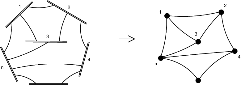
Then, the correlation function (3.22) is given by a set of diagrams in which an arbitrary number of propagators are stretched between $n$ lines, or equivalently connect $n$ effective vertices (see Fig. 2).

Let us consider the propagator connecting two lines with indices $i$ and $j$ . Denoting the local parameters of the points on these two lines by $\sigma_{ij}^{\alpha}$ and $\sigma_{ji}^{\alpha}$ , respectively, we can write its contribution as

		$\displaystyle{}\int\langle{\sigma_{ij}d\sigma_{ij}}\rangle\int\langle{\sigma_{ji}d\sigma_{ji}}\rangle\,\delta^{2\|4}(\mathcal{Z}_{i}(\sigma_{ij}),\mathcal{Z}_{j}(\sigma_{ji}),\mathcal{Z}_{*})(\dots)$
		$\displaystyle{}\qquad=\int\langle{\sigma_{ij}d\sigma_{ij}}\rangle\int\langle{\sigma_{ji}d\sigma_{ji}}\rangle\int{ds\over s}{dt\over t}\,\delta^{4\|4}(s\mathcal{Z}_{i}(\sigma_{ij})+t\mathcal{Z}_{j}(\sigma_{ji})+\mathcal{Z}_{*})(\dots)$
		$\displaystyle{}\qquad=\int d^{2}\sigma_{ij}\int d^{2}\sigma_{ji}\,\delta^{4\|4}({\cal Z}_{*}+\sigma_{ij}^{\alpha}{\cal Z}_{i,\alpha}+\sigma_{ji}^{\alpha}{\cal Z}_{j,\alpha})(\dots)\,,$		(3.24)

where the expression inside $(\dots)$ corresponds to the rest of the diagram and we made use of (3.14) in the second relation. Here in the third relation we replaced the integration variables $\sigma^{\alpha}_{ij}\to s\sigma^{\alpha}_{ij}$ and $\sigma^{\alpha}_{ji}\to t\sigma^{\alpha}_{ji}$ taking into account that the expression inside $(\dots)$ is a homogenous function of $\sigma_{ij}$ and $\sigma_{ji}$ of degree $(-2)$ .

Then, the Feynman rules taking us from a graph as shown in Fig. 2 to a contribution to the correlation function (3.22) are as follows:

•

To each line connecting vertices $i$ and $j$ we associate two pairs of spinor variables $\sigma_{ij}^{\alpha}$ and $\sigma_{ji}^{\alpha}$ (with $\alpha=1,2$ ). They define the coordinates of the end points $\sigma_{ij}^{\alpha}{\cal Z}_{i,\alpha}$ and $\sigma_{ji}^{\alpha}{\cal Z}_{j,\alpha}$ belonging to the $i$ th and $j$ th lines, respectively, in projective twistor space ⁸⁸ 8 Such an assignment of the $\sigma_{ij}$ variables would be ambiguous if two vertices were connected by more than one line. As we show below (see Eq. (3.49)), this never happens for $n-$ point correlation functions if $n>2$ .;
•

A propagator connecting vertices $i$ and $j$ produces a graded delta function $\delta^{a_{i}a_{j}}\delta^{4|4}({\cal Z}_{*}+\sigma_{ij}^{\alpha}{\cal Z}_{i,\alpha}+\sigma_{ji}^{\alpha}{\cal Z}_{j,\alpha})$ with $a_{i}$ and $a_{j}$ being $SU(N)$ colour indices;
•

Each vertex comes with a Parke-Taylor-like denominator accompanied by the $SU(N)$ colour factor, $-\mathop{\rm tr}\nolimits[T^{a_{j_{1}}}T^{a_{j_{2}}}\cdots T^{a_{j_{k}}}]/\prod_{\ell=1}^{k}\langle{\sigma_{ij_{\ell}}\sigma_{ij_{\ell+1}}}\rangle$ (with $j_{k+1}\equiv j_{1}$ and $\langle{\sigma_{ij_{\ell}}\sigma_{ij_{\ell+1}}}\rangle$ given by (3.16)). In virtue of $\mathop{\rm tr}\nolimits T^{a_{j}}=0\phantom{{}^{\beta}}$ , we must have at least two lines coming from each vertex;
•

Finally, at each vertex $i=1,\dots,n$ we have to perform an integration $\int d^{2}\sigma_{ij_{1}}\dots d^{2}\sigma_{ij_{k}}$ over the $\sigma-$ parameters of all lines attached to that vertex and, in addition, integrate out half of the Grassmann variables by $\int d^{4}\theta_{i}^{-}$ .

These rules are summarised in Fig. 3.

To compute an $n-$ point correlation function using these Feynman rules we have to examine all diagrams with exactly $n$ vertices and an arbitrary number of propagators. Since each vertex has at least two lines attached to it, the minimal number of propagators is $n$ . Let us denote the total number of propagators as $n+p$ (with $p\geq 0$ ) and examine the Grassmann degree of the corresponding diagram. Each propagator increases the Grassmann degree by four units whereas each vertex reduces it by four units due to the integration $\int d^{4}\theta_{i}^{-}$ . Thus, the Grassmann degree of a diagram containing $n$ vertices and $n+p$ propagators is $4\,p$ . This counting is in perfect agreement with the general form of the correlation function (1.1). It also allows us to identify each term in the expansion (1.1) with the contribution of a particular class of diagrams:

\displaystyle G_{n;p}=\text{Sum of diagrams with $n$ vertices and $n+p$ propagators}

(3.25)

3.4 Lowest component

To illustrate the formalism, we apply the Feynman rules formulated in the previous subsection to compute the simplest $G_{n;0}$ component of the correlation function (1.1). According to (3.25), $G_{n;0}$ is given by the sum of diagrams with $n$ vertices and $n$ propagators. A distinctive feature of such diagrams is that all vertices are bivalent. In what follows we shall only consider connected twistor diagrams. ⁹⁹ 9 The disconnected twistor diagrams describe contributions to the correlation function which reduce to products of correlators with lower number of points. A particular example of such a diagram is the graph in which vertices $i$ and $i+1$ are connected by a single line. All remaining diagrams can be obtained by permuting the labels of the vertices. According to the Feynman rules in Fig. 1, the contribution of the $i$ th vertex involves $-1/(\langle{\sigma_{i,i-1}\sigma_{i,i+1}}\rangle\langle{\sigma_{i,i+1}\sigma_{i,i-1}}\rangle)=1/\langle{\sigma_{i,i-1}\sigma_{i,i+1}}\rangle^{2}$ . We combine it with the propagators to obtain ¹⁰¹⁰ 10 Here we do not display the factor $(N^{2}-1)$ coming from the contraction of the $SU(N)$ colour indices since it is included in (2.6).

\displaystyle G_{n;0}=\prod_{i=1}^{n}\int d^{4}\theta_{i}^{-}\int{d^{2}\sigma_{i,i-1}d^{2}\sigma_{i,i+1}\over\langle{\sigma_{i,i-1}\sigma_{i,i+1}}\rangle^{2}}\delta^{4|4}({\cal Z}_{*}+\sigma_{i,i-1}^{\beta}{\cal Z}_{i,\beta}+\sigma_{i-1,i}^{\beta}{\cal Z}_{i-1,\beta})+\text{($S_{n}-$perm)},

(3.26)

where ( $S_{n}-$ perm) denotes the additional terms needed to restore the Bose symmetry of the correlation function.

We recall that ${\cal Z}_{i,1}$ and ${\cal Z}_{i,2}$ denote two points on a line in supertwistor space. They have the general form (3.8) and (3.9) with the local coordinates $\lambda_{1,\beta}$ and $\lambda_{2,\beta}$ , respectively. The correlation function (3.26) should not depend on the choice of these coordinates. Indeed, the change of the local coordinates corresponds to the $GL(2)$ rotation $\lambda_{\gamma,\beta}\to g_{\gamma}{}^{\delta}\lambda_{\gamma,\beta}$ , or equivalently ${\cal Z}_{i,\beta}\to g_{\gamma}{}^{\delta}{\cal Z}_{i,\delta}$ . This variation can be compensated in (3.26) by the change of the integration variable $\sigma_{ik}^{\beta}\to(g^{-1})^{\beta}{}_{\delta}\sigma_{ik}^{\delta}$ . We can make use of this symmetry to choose ${\cal Z}_{i,\beta}$ in the following form

\displaystyle{\cal Z}_{i,\beta}=(Z_{i,\beta}^{\,I},\ \theta^{\,A}_{i,\beta})\,,\qquad\qquad Z_{i,\beta}^{\,I}=(\epsilon_{\alpha\beta},\ ix_{i,\beta}^{\,\dot{\alpha}})\,,

(3.27)

with $I=(\alpha,\dot{\alpha})$ . It is also convenient to parameterise the axial gauge supertwistor as

\displaystyle{\cal Z}_{*}=(Z_{*}^{\,I},\ \theta^{\,A}_{*})\,.

(3.28)

We substitute (3.27) into (3.26) and perform the integration over $\theta_{i}^{-}$ to obtain (see Eq. (3.34) below)

\displaystyle G_{n;0}=\prod_{i=1}^{n}\,y_{i,i+1}^{2}\int{d^{2}\sigma_{i,i-1}d^{2}\sigma_{i,i+1}}\delta^{4}(Z_{*}+\sigma_{i,i-1}^{\beta}Z_{i,\beta}+\sigma_{i-1,i}^{\beta}Z_{i-1,\beta})+\text{($S_{n}-$perm)}\,.

(3.29)

Here $y_{i,i+1}=y_{i}-y_{i+1}$ with $y_{i}$ being the local coordinates on the harmonic coset introduced in (A.5). We notice that the total number of delta functions in this integral matches the number of integration variables. Therefore, the integral is localised at the values of the $\sigma-$ parameters satisfying $Z_{*}+\sigma_{i,i-1}^{\beta}Z_{i,\beta}+\sigma_{i-1,i}^{\beta}Z_{i-1,\beta}=0$ . Equivalently

		$\displaystyle\sigma_{i,i-1}^{\alpha}=\epsilon^{\alpha\beta}{\langle{Z_{i,\beta}Z_{*}Z_{i-1,1}Z_{i-1,2}}\rangle\over\langle{Z_{i-1,1}Z_{i-1,2}Z_{i,1}Z_{i,2}}\rangle}\,,$
		$\displaystyle\sigma_{i-1,i}^{\alpha}=\epsilon^{\alpha\beta}{\langle{Z_{i-1,\beta}Z_{*}Z_{i,1}Z_{i,2}}\rangle\over\langle{Z_{i-1,1}Z_{i-1,2}Z_{i,1}Z_{i,2}}\rangle}\,,$		(3.30)

where we used the notation $\langle{Z_{1}Z_{2}Z_{3}Z_{4}}\rangle=\epsilon_{IJKL}Z_{1}^{I}Z_{2}^{J}Z_{3}^{K}Z_{4}^{L}$ . In this way, we finally obtain

\displaystyle G_{n;0}=\prod_{i=1}^{n}\,{y_{i,i+1}^{2}\over x_{i,i+1}^{2}}+\text{($S_{n}-$perm)}\,.

(3.31)

Notice that the dependence on the reference supertwistor ${\cal Z}_{*}$ disappeared in $G_{n;0}$ as it should for a gauge invariant quantity.

The result (3.31) perfectly meets our expectations. In the conventional approach, $G_{n;0}$ coincides with the correlation function of $n$ operators $\mathop{\rm tr}\nolimits[\phi^{++}\phi^{++}]$ , the lowest component of the stress-tensor multiplet (2.2). Then, to lowest order in the coupling constant, $G_{n;0}$ is given by a product of $n$ free scalar propagators $\langle{\phi^{++}(i)\phi^{++}(j)}\rangle=y_{ij}^{2}/x_{ij}^{2}$ , properly symmetrised to respect Bose symmetry.

3.5 Twistor Feynman rules for higher components

To compute higher components of the correlation function $G_{n;p}$ we have to examine all diagrams containing $n$ vertices and $n+p$ propagators. We can apply the Feynman rules formulated in the previous sections to write down their contribution as a productsof $n+p$ graded delta functions of the form $\delta^{4|4}({\cal Z}_{*}+\sigma_{ij}^{\alpha}{\cal Z}_{i,\alpha}+\sigma_{ji}^{\alpha}{\cal Z}_{j,\alpha})$ . However, this approach is not very efficient in that it involves integrating a function of Grassmann degree $4(n+p)$ over $4n$ odd variables $\int d^{4}\theta_{i}^{-}$ to arrive at the function $G_{n;p}$ of Grassmann degree $4p$ . So, in this subsection we instead perform the explicit integration over the variables $\theta_{i}^{-}$ at the level of the twistor Feynman rules and thus derive a simpler set of rules.

To begin with, we split each propagator up into a product of bosonic and fermionic delta functions,

\displaystyle\delta^{4}(Z_{*}+\sigma_{ij}^{\alpha}Z_{i,\alpha}+\sigma_{ji}^{\alpha}Z_{j,\alpha})\delta^{4}(\theta_{*}+\sigma_{ij}^{\alpha}\theta_{i,\alpha}+\sigma_{ji}^{\alpha}\theta_{j,\alpha})\,.

(3.32)

To integrate over $\theta_{i}^{-}$ , we employ the harmonics $u_{i}$ to decompose the variables $\theta_{i}$ into two halves (3.20) (see Appendix A),

\displaystyle\theta^{A}_{i}=\theta_{i}^{+a}\bar{u}_{i,+a}^{A}+\theta_{i}^{-a^{\prime}}\bar{u}_{i,-a^{\prime}}^{A}\,.

(3.33)

Then, multiplying the argument of the fermionic delta function by the $4\times 2$ matrices $u_{i,A}^{+a}$ and $u_{j,A}^{+a}$ we find after some algebra

\displaystyle\delta^{4}(\theta_{*}+\langle{\sigma_{ij}\theta_{i}}\rangle+\langle{\sigma_{ji}\theta_{j}}\rangle)=y_{ij}^{2}\,\delta^{2}\left(\langle{\sigma_{ij}\theta_{i}^{-}}\rangle+A_{ij}\right)\delta^{2}\left(\langle{\sigma_{ji}\theta_{j}^{-}}\rangle+A_{ji}\right)\,,

(3.34)

with $y_{ij}^{2}=\frac{1}{4}\epsilon^{ABCD}u_{i,A}^{+a}\epsilon_{ab}u_{i,B}^{+b}u_{j,C}^{+c}\epsilon_{cd}u_{j,D}^{+d}$ . Here the functions

\displaystyle A_{ij}^{a^{\prime}}=\left[\langle{\sigma_{ji}\theta_{j}^{+b}}\rangle+\langle{\sigma_{ij}\theta_{i}^{+c}}\rangle(U_{ij})_{+c}^{+b}+\theta_{*}^{A}u_{j,A}^{+b}\right](U_{ij}^{-1})_{+b}^{-a^{\prime}}

(3.35)

depend only on $\theta^{+}_{i}$ and $\theta^{+}_{j}$ , and the matrices $U_{ij}$ are defined as

\displaystyle(U_{ij})_{+c}^{+b}=\bar{u}_{i,+c}^{A}u_{j,A}^{+b}\,,\qquad\qquad(U_{ij})_{-a^{\prime}}^{+b}=\bar{u}_{i,-a^{\prime}}^{A}u_{j,A}^{+b}\,.

(3.36)

The function $A_{ji}^{a^{\prime}}$ can be obtained from $A_{ij}^{a^{\prime}}$ by exchanging the indices $i\leftrightarrow j$ . It is often convenient to use a parameterisation of the harmonic variables $u_{i}$ in terms of the local coordinates $y_{i}$ on the harmonic coset defined in (A.5). In this case, $(U_{ij})_{+c}^{+b}=\delta_{c}^{b}$ and $(U_{ij})_{-a^{\prime}}^{+b}=(y_{ij})_{a^{\prime}}^{b}$ , so that the expression (3.35) significantly simplifies,

\displaystyle A_{ij}^{a^{\prime}}=\left[\langle{\sigma_{ji}\theta_{j}^{+b}}\rangle+\langle{\sigma_{ij}\theta_{i}^{+b}}\rangle+\theta_{*}^{A}u_{j,A}^{+b}\right](y_{ij}^{-1})_{b}^{a^{\prime}}\,.

(3.37)

Notice that the dependence on $\theta^{-}_{i}$ and $\theta^{-}_{j}$ on the right-hand side of (3.34) resides in the first and second delta functions, respectively. This suggests associating the first delta function with the vertex $i$ and the second one with the vertex $j$ . Then, if the vertex $i$ has $k$ propagators attached to it, we take into account the additional $\sigma-$ dependent factor coming from the Feynman rules in Fig. 3 to arrive at the integral

\displaystyle R(i;j_{1}j_{2}\dots j_{k})=-\int d^{4}{\theta^{-}_{i}}{\delta^{2}(\langle{\sigma_{ij_{1}}\theta^{-}_{i}}\rangle+A_{ij_{1}})\delta^{2}(\langle{\sigma_{ij_{2}}\theta^{-}_{i}}\rangle+A_{ij_{2}})\dots\delta^{2}(\langle{\sigma_{ij_{k}}\theta^{-}_{i}}\rangle+A_{ij_{k}})\over\langle{\sigma_{ij_{1}}\sigma_{ij_{2}}}\rangle\,\langle{\sigma_{ij_{2}}\sigma_{ij_{3}}}\rangle\,\dots\,\langle{\sigma_{ij_{k}}\sigma_{ij_{1}}}\rangle}\ .

(3.38)

Here the index $i$ labels the vertex and the indices $j_{1},\dots,j_{k}$ enumerate the outgoing lines. By construction, this integral has Grassmann degree $(2k-4)$ . As we shall see in the next section, the quantity $R(i;j_{1}j_{2}\dots j_{k})$ plays a crucial role in our analysis.

Relation (3.38) depends on the parameters $\sigma_{ij}^{\alpha}$ and $\sigma_{ji}^{\alpha}$ . Their values can be determined using the bosonic part of the propagator (3.32). Namely, solving the equation $Z_{*}^{I}+\langle{\sigma_{ij}Z_{i}^{I}}\rangle+\langle{\sigma_{ji}Z_{j}^{I}}\rangle=0$ we obtain

\displaystyle\sigma_{ij}^{\alpha}=\epsilon^{\alpha\beta}{\langle{Z_{i,\beta}Z_{*}Z_{j,1}Z_{j,2}}\rangle\over\langle{Z_{i,1}Z_{i,2}Z_{j,1}Z_{j,2}}\rangle}\,,\qquad\qquad\sigma_{ji}^{\alpha}=\epsilon^{\alpha\beta}{\langle{Z_{j,\beta}Z_{*}Z_{i,1}Z_{i,2}}\rangle\over\langle{Z_{i,1}Z_{i,2}Z_{j,1}Z_{j,2}}\rangle}\,,

(3.39)

c.f. (3.30). Finally, for each propagator (3.32) the bosonic delta function allows us to do the $\sigma-$ integration yielding

\displaystyle y_{ij}^{2}\int d^{2}\sigma_{ij}d^{2}\sigma_{ji}\,\delta^{4|0}(Z^{*}+\sigma_{ij}Z_{i}+\sigma_{ji}Z_{j})={y_{ij}^{2}\over\langle{Z_{i,1}Z_{i,2}Z_{j,1}Z_{j,2}}\rangle}={y_{ij}^{2}\over x_{ij}^{2}}\ ,

(3.40)

where the additional factor of $y_{ij}^{2}$ comes from (3.34).

In summary, we arrive at the following twistor Feynman rules shown in Fig. 4:

•

A line connecting vertices $i$ and $j$ is associated with the propagator $d_{ij}=y_{ij}^{2}/x_{ij}^{2}$ ;
•

Bivalent vertices are associated with $R(i;j_{1}j_{2})\mathop{\rm tr}\nolimits[T^{a_{j_{1}}}T^{a_{j_{2}}}]=R(i;j_{1}j_{2})\delta^{a_{j_{1}}a_{j_{2}}}$ ;
•

Higher valency vertices are associated with $R(i;j_{1}\dots j_{k})\mathop{\rm tr}\nolimits[T^{a_{j_{1}}}\dots T^{a_{j_{k}}}]$ evaluated for the $\sigma-$ parameters given by (3.39).

Figure 4: Feynman rules for propagators and vertices in analytic superspace.

3.6 Properties of the $R-$ vertices

Let us summarise the properties of $R(i;j_{1}j_{2}\dots j_{k})$ . In twistor diagrams, this function is accompanied by the colour factor $\mathop{\rm tr}\nolimits[T^{a_{j_{1}}}\dots T^{a_{j_{k}}}]$ with the same ordering of external lines. As follows from the representation (3.38), $R(i;j_{1}j_{2}\dots j_{k})$ is invariant under a cyclic shift of the $j-$ indices and changes sign under a ‘mirror’ exchange of the indices, $j_{\ell}\to j_{k-\ell+1}$ ,

\displaystyle R(i;j_{1}j_{2}\dots j_{k-1}j_{k})=R(i;j_{2}j_{3}\dots j_{k}j_{1})=(-1)^{k}R(i;j_{k}j_{k-1}\dots j_{2}j_{1})\,.

(3.41)

For $k=3$ external lines, this relation implies that $R(i;j_{1}j_{2}j_{3})$ is completely antisymmetric under the exchange of external legs,

\displaystyle R(i;j_{1}j_{2}j_{3})=-R(i;j_{1}j_{3}j_{2})=-R(i;j_{3}j_{2}j_{1})=R(i;j_{2}j_{3}j_{1})\,.

(3.42)

In the special case $j_{2}=j_{3}$ , corresponding to a graph in which the two external legs are attached to the same vertex, this relation implies

\displaystyle R(i;j_{1}j_{2}j_{2})=0\,.

(3.43)

Let us examine the explicit expression for $R(i;j_{1}j_{2}\dots j_{k})$ for the lowest values of $k$ . For a bivalent vertex, $k=2$ , the integration in (3.38) yields

\displaystyle R(i;j_{1}j_{2})=1\,.

(3.44)

For a valency three vertex, $k=3$ , we can make use of the Schouten identity

\displaystyle\sigma_{ij_{1}}^{\alpha}\langle\sigma_{ij_{2}}\sigma_{ik}\rangle+\sigma_{ij_{2}}^{\alpha}\langle\sigma_{ik}\sigma_{ij_{1}}\rangle+\sigma_{ik}^{\alpha}\langle\sigma_{ij_{1}}\sigma_{ij_{2}}\rangle=0\

(3.45)

to rewrite the argument of one of the three delta functions on the support of the other two in such a way that it becomes $\theta^{-}_{i}$ independent. In this way, we obtain

\displaystyle R(i;j_{1}j_{2}j_{3})=-{\delta^{2}\Big(\langle\sigma_{ij_{1}}\sigma_{ij_{2}}\rangle A_{ij_{3}}+\langle\sigma_{ij_{2}}\sigma_{ij_{3}}\rangle A_{ij_{1}}+\langle\sigma_{ij_{3}}\sigma_{ij_{1}}\rangle A_{ij_{2}}\Big)\over\langle{\sigma_{ij_{1}}\sigma_{ij_{2}}}\rangle\,\langle{\sigma_{ij_{2}}\sigma_{ij_{3}}}\rangle\,\langle{\sigma_{ij_{3}}\sigma_{ij_{1}}}\rangle}\ .

(3.46)

For vertices of higher valency, we can recursively apply the same trick, reducing a $k-$ valent vertex to a product of $3-$ and $(k-1)-$ valent vertices. Specifically, we rewrite the last delta function on the right-hand side of (3.38) as a combination of the first and the $(k-1)$ st to get

\displaystyle R(i;j_{1}j_{2}\dots j_{k})=R(i;j_{1}j_{2}\dots j_{k-1})\,R(i;j_{1}j_{k-1}j_{k})\ .

(3.47)

Continuing recursively we can express the $k-$ valent vertex as a product of $(k-2)$ copies of $3-$ valent vertices

\displaystyle R(i;j_{1}j_{2}\dots j_{k})=R(i;j_{1}j_{2}j_{3})\,R(i;j_{1}j_{3}j_{4})\,\dots\,R(i;j_{1}j_{k-1}j_{k})\ .

(3.48)

Note that the index $j_{1}$ plays a special role here as it appears in every factor on the right-hand side. We can obtain another equivalent representation for $R(i;j_{1}j_{2}\dots j_{k})$ by making use of the symmetry properties (3.41). Combining (3.48) with (3.43) we find that the $R-$ vertex vanishes if two indices of external lines coincide

\displaystyle R(i;j_{1}j_{1}j_{3}\dots j_{k})=R(i;j_{1}j_{2}\dots j_{1}\dots j_{k})=0\,.

(3.49)

In terms of twistor diagrams this relation implies that diagrams with (at least) two propagators stretched between any two twistor lines do not contribute to the correlation function.

We observe that the denominator in (3.38) has the same form as in the Parke-Taylor MHV amplitude upon identifying the variables $\sigma_{ij}$ with the holomorphic variables $\lambda_{j}$ that define the on-shell momenta of the particles. As a consequence, we can use the properties of the MHV amplitude to obtain non-trivial relations for $R(i;j_{1}j_{2}\dots j_{k})$ . In particular, the $U(1)$ decoupling relation for MHV amplitudes [28] translates into

\displaystyle R(i;j_{1}j_{2}\dots j_{k-1}j_{k})+R(i;j_{1}j_{3}\dots j_{k}j_{2})+\dots+R(i;j_{1}j_{k}\dots j_{k-2}j_{k-1})=0\,,

(3.50)

where the sum runs over cyclic permutations of the indices $j_{2},\dots,j_{k-1},j_{k}$ . This relation can be verified using the Schouten identity (3.45).

The $R-$ vertices satisfy another set of non-trivial relations. In the simplest case of three-point vertices it takes the form

\displaystyle R(i;j_{1}j_{2}j_{3})=R(i;j_{4}j_{2}j_{3})+R(i;j_{1}j_{4}j_{3})+R(i;j_{1}j_{2}j_{4})\,,

(3.51)

with $j_{1},\dots,j_{4}$ being arbitrary. The proof of this relation can be found in Appendix B. We can then use (3.51) and (3.48) together to obtain an analogous relation for four points

	$\displaystyle R(i;j_{1}j_{2}j_{3}j_{4}){}$	$\displaystyle=R(i;j_{5}j_{2}j_{3}j_{4})+R(i;j_{1}j_{5}j_{3}j_{4})+R(i;j_{1}j_{2}j_{5}j_{4})+R(i;j_{1}j_{2}j_{3}j_{5})$
		$\displaystyle+R(i;j_{5}j_{1}j_{2})R(i;j_{5}j_{3}j_{4})+R(i;j_{5}j_{2}j_{3})R(i;j_{5}j_{4}j_{1})\,.$		(3.52)

It is straightforward to generalise it to an arbitrary number of points

\displaystyle R(i;j_{1}j_{2}\dots j_{k})=R(i;j_{k+1}j_{2}\dots j_{k})+\frac{1}{2}\sum_{p=2}^{k-2}R(i;j_{k+1}j_{1}\dots j_{p})R(i;j_{k+1}j_{p+1}\dots j_{k})+\text{cyclic($j_{1}j_{2}\dots j_{k}$)}\,,

(3.53)

where the expression on the right-hand side is symmetrised with respect to cyclic permutations of the indices $j_{1},j_{2},\dots,j_{k}$ .

4 Next-to-lowest component

As we have shown in the previous section, the lowest component of the correlation function (1.1) reduces to a product of free scalar propagators (3.31). In this section, we shall compute the first component $G_{n;1}$ of (1.1) with non-trivial dependence on the Grassmann variables. We recall that $G_{n;1}$ is a homogenous function of $\theta_{i}^{+}$ (with $i=1,\dots,n$ ) of degree four.

In the conventional approach, to obtain $G_{n;1}$ we have to replace the superfields $\mathcal{T}(i)$ in (2.3) by their expansion (2.2) in powers of $\theta^{+}_{i}$ and to single out the contribution involving products of four Grassmann variables. In this way, $G_{n;1}$ is given by a sum of $n-$ point correlation functions involving various components of the stress-tensor supermultiplet. Each of these component correlation functions has conformal symmetry, but ${\cal N}=4$ supersymmetry is not manifest. The main advantage of the twistor space approach is to offer an efficient way of finding $G_{n;1}$ without the need of computing individual component correlation functions; ${\cal N}=4$ supersymmetry is manifest.¹¹¹¹ 11 We recall that the price to pay for this is the presence of the reference twistor ${\cal Z}_{*}$ , in addition to the external data. The important point however is that ${\cal Z}_{*}$ drops out from the final expressions, due to gauge invariance.

According to (3.25), the correlation function $G_{n;1}$ is given by the sum of all twistor diagrams containing $n$ vertices and $(n+1)$ edges. Since each vertex is at least $2-$ valent, such diagrams may have either two $3-$ valent vertices, or a single $4-$ valent vertex with the remaining vertices being $2-$ valent. Thus, we distinguish different topologies of twistor diagrams shown in Fig. 5. The last three diagrams correspond to different embeddings of the colour-ordered quartic vertex.

Let us first consider the contribution of the diagram shown in Fig. 5(a). It involves two chains of propagators attached to two cubic vertices with indices $i$ and $j_{3}$ . Applying the Feynman rules, we find that the contribution of this diagram to the correlation function vanishes

\displaystyle G_{n;1}^{\text{(a)}}\sim\delta^{a_{j_{1}}a_{j_{2}}}\mathop{\rm tr}\nolimits[T^{a_{j_{1}}}T^{a_{j_{2}}}T^{a_{j_{3}}}]R(i;j_{1}j_{2}j_{3})=0\,,

(4.1)

where $\delta^{a_{j_{1}}a_{j_{2}}}$ comes from the product of propagators connecting $2-$ valent vertices $j_{1}$ and $j_{2}$ . Here we took into account that $T^{a}T^{a}=C_{F}=(N^{2}-1)/N$ is the quadratic Casimir of the gauge group $SU(N)$ and, as a consequence, the colour trace in the above relation vanishes, $\mathop{\rm tr}\nolimits T^{a_{j_{3}}}=0$ .

The diagram shown in Fig. 5(b) contains three chains of propagators attached to two vertices with indices $i$ and $j$ . Explicitly, its contribution is

	$\displaystyle{\rm Fig.~\ref{fig-topos}(b)}={}$	$\displaystyle R(i;k_{1}l_{1}m_{1})\mathop{\rm tr}\nolimits[T^{a_{k_{1}}}T^{a_{l_{1}}}T^{a_{m_{1}}}]\times R(j;k_{2}l_{2}m_{2})\mathop{\rm tr}\nolimits[T^{a_{k_{2}}}T^{a_{l_{2}}}T^{a_{m_{2}}}]$
	$\displaystyle\times$	$\displaystyle\delta^{a_{k_{1}}a_{k_{2}}}\left({y_{ik_{1}}^{2}\over x_{ik_{1}}^{2}}\dots{y_{k_{2}j}^{2}\over x_{k_{2}j}^{2}}\right)\times\delta^{a_{l_{1}}a_{l_{2}}}\left({y_{il_{1}}^{2}\over x_{il_{1}}^{2}}\dots{y_{l_{2}j}^{2}\over x_{l_{2}j}^{2}}\right)\times\delta^{a_{m_{1}}a_{m_{2}}}\left({y_{im_{1}}^{2}\over x_{im_{1}}^{2}}\dots{y_{m_{2}j}^{2}\over x_{m_{2}j}^{2}}\right)\,,$		(4.2)

where the dots stand for the product of the remaining propagators constituting the three chains. As opposed to the previous case, the colour factor of this diagram is different from zero. In the correlation function, the above expression should be symmetrised with respect to the indices of all vertices in order to respect the Bose symmetry. In particular, since the cubic vertex is antisymmetric under the exchange of external legs, $R(i;k_{1}l_{1}m_{1})=-R(i;l_{1}k_{1}m_{1})$ , its colour factor $\mathop{\rm tr}\nolimits[T^{a_{k_{1}}}T^{a_{l_{1}}}T^{a_{m_{1}}}]$ should also have the same property for the contribution of the diagram to be Bose symmetric. This allows us to replace $\mathop{\rm tr}\nolimits(T^{a_{k_{1}}}T^{a_{l_{1}}}T^{a_{m_{1}}})\to\mathop{\rm tr}\nolimits([T^{a_{k_{1}}},T^{a_{l_{1}}}]T^{a_{m_{1}}})$ yielding

\displaystyle\delta^{a_{k_{1}}a_{k_{2}}}\delta^{a_{l_{1}}a_{l_{2}}}\delta^{a_{m_{1}}a_{m_{2}}}\mathop{\rm tr}\nolimits\left([T^{a_{k_{1}}},T^{a_{l_{1}}}]T^{a_{m_{1}}}\right)\mathop{\rm tr}\nolimits\left([T^{a_{k_{2}}},T^{a_{l_{2}}}]T^{a_{m_{2}}}\right)=-2(N^{2}-1)N\,,

(4.3)

where we used $[T^{a},T^{b}]=i\sqrt{2}f^{abc}T^{c}$ with $f^{abc}f^{abc^{\prime}}=N\delta^{cc^{\prime}}$ for the gauge group $SU(N)$ and $\mathop{\rm tr}\nolimits(T^{a}T^{b})=\delta^{ab}$ . In this way, we find the contribution of the diagram in Fig. 5(b) (see footnote 10)

\displaystyle G_{n;1}^{\rm(b)}=-R(i;k_{1}l_{1}m_{1})R(j;k_{2}l_{2}m_{2})d_{ik_{1}\dots k_{2}j}d_{il_{1}\dots l_{2}j}d_{im_{1}\dots m_{2}j}+\text{($S_{n}-$perm)}\,,

(4.4)

where the notation was introduced for the product of scalar propagators

\displaystyle d_{ik_{1}\dots k_{2}j}={y_{ik_{1}}^{2}\over x_{ik_{1}}^{2}}\dots{y_{k_{2}j}^{2}\over x_{k_{2}j}^{2}}\,.

(4.5)

The diagrams shown in Fig. 5(c)–(e) contain two chains of propagators that are attached to the quartic vertex in three different ways. Their contribution to the correlation function is

\displaystyle\text{Fig.~\ref{fig-topos}(c+d+e)}=d_{ij_{1}\dots j_{2}i}{}

\displaystyle d_{ij_{4}\dots j_{3}i}\big[C_{\rm c}\,R(i;j_{1}j_{2}j_{3}j_{4})+C_{\rm d}\,R(i;j_{1}j_{3}j_{4}j_{2})+C_{\rm e}\,R(i;j_{1}j_{4}j_{2}j_{3})\big]\,.

(4.6)

The colour factors are

$\displaystyle C_{\rm c}$	$\displaystyle=\delta^{a_{j_{1}}a_{j_{2}}}\delta^{a_{j_{3}}a_{j_{4}}}\mathop{\rm tr}\nolimits{\left({T^{a_{j_{1}}}T^{a_{j_{2}}}T^{a_{j_{3}}}T^{a_{j_{4}}}}\right)}=NC_{F}^{2}\,,$
$\displaystyle C_{\rm d}$	$\displaystyle=\delta^{a_{j_{1}}a_{j_{2}}}\delta^{a_{j_{3}}a_{j_{4}}}\mathop{\rm tr}\nolimits{\left({T^{a_{j_{2}}}T^{a_{j_{1}}}T^{a_{j_{3}}}T^{a_{j_{4}}}}\right)}=NC_{F}^{2}\,,$
$\displaystyle C_{\rm e}$	$\displaystyle=\delta^{a_{j_{1}}a_{j_{2}}}\delta^{a_{j_{3}}a_{j_{4}}}\mathop{\rm tr}\nolimits{\left({T^{a_{j_{1}}}T^{a_{j_{4}}}T^{a_{j_{2}}}T^{a_{j_{3}}}}\right)}=NC_{F}(C_{F}-N)\,,$	(4.7)

where $C_{F}=(N^{2}-1)/N$ is the quadratic Casimir of $SU(N)$ in the fundamental representation. Notice that $C_{\rm e}$ is suppressed at large $N$ by a factor of $1/N^{2}$ , compared to $C_{\rm c}$ and $C_{\rm d}$ . This reflects the fact that the former diagram is non-planar whereas the latter two are planar.

Substituting (4.7) into (4.6) we expect to encounter both planar and non-planar contributions. It turns out that the non-planar diagram 5(e) cancels against the $1/N^{2}$ suppressed contributions of the diagrams in Fig. 5(c)+(d) in such a way that their total sum remains planar in the large $N$ limit, in perfect agreement with (2.6). To show this, we apply the relation (3.50) for $k=4$ to replace $R(i;j_{1}j_{4}j_{2}j_{3})=-R(i;j_{1}j_{2}j_{3}j_{4})-R(i;j_{1}j_{3}j_{4}j_{2})$ in (4.6) leading to

		$\displaystyle C_{\rm c}\,R(i;j_{1}j_{2}j_{3}j_{4})+C_{\rm d}\,R(i;j_{1}j_{3}j_{4}j_{2})+C_{\rm e}\,R(i;j_{1}j_{4}j_{2}j_{3})$
		$\displaystyle\qquad=(C_{\rm c}-C_{\rm e})R(i;j_{1}j_{2}j_{3}j_{4})+(C_{\rm d}-C_{\rm e})R(i;j_{1}j_{3}j_{4}j_{2})$
		$\displaystyle\qquad=(N^{2}-1)N\big[R(i;j_{1}j_{2}j_{3}j_{4})+R(i;j_{2}j_{1}j_{3}j_{4})\big]\,,$		(4.8)

where in the last relation we made use of the identity $R(i;j_{1}j_{3}j_{4}j_{2})=R(i;j_{2}j_{1}j_{3}j_{4})$ , Eq. (3.41). Comparing with (4.7) we observe that all terms proportional to $C_{F}^{2}$ cancel out in the sum over all diagrams and the only terms that survive are those involving the colour factor $C_{F}N$ . This property is reminiscent of the so-called non-abelian exponentiation of Wilson loops [29, 30].

We combine (4.6) and (4.8) to obtain the contribution of the diagrams Fig. 5(c),(d),(e) to the correlation function (see footnote 10)

\displaystyle G_{n;1}^{\text{(c)+(d)+(e)}}=R(i;j_{1}j_{2}j_{3}j_{4})\,d_{ij_{1}\dots j_{2}i}{}

\displaystyle d_{ij_{4}\dots j_{3}i}+\text{($S_{n}-$perm)}\,.

(4.9)

This expression involves a quartic vertex which can be expressed in terms of cubic vertices using (3.48)

\displaystyle R(i;j_{1}j_{2}j_{3}j_{4})=R(i;j_{1}j_{2}j_{3})\,R(i;j_{1}j_{3}j_{4})=R(i;j_{2}j_{4}j_{1})\,R(i;j_{2}j_{3}j_{4})\ .

(4.10)

Finally, we combine relations (4.1), (4.4) and (4.9) to obtain the following representation for the next-to-lowest component of the correlation function:

	$\displaystyle G_{n;1}={}$	$\displaystyle-R(i;k_{1}l_{1}m_{1})R(j;k_{2}l_{2}m_{2})d_{ik_{1}\dots k_{2}j}d_{il_{1}\dots l_{2}j}d_{im_{1}\dots m_{2}j}$
		$\displaystyle+R(i;j_{1}j_{2}j_{3})\,R(i;j_{1}j_{3}j_{4})d_{ij_{1}\dots j_{2}i}d_{ij_{4}\dots j_{3}i}+\text{($S_{n}-$perm)}\,.$		(4.11)

Here the indices $i,j,k,l,m$ label $n$ different points and the sum runs over their permutations.

The following comments are in order concerning the properties of (4.11).

A remarkable feature of (4.11) is that the whole dependence on the Grassmann variables is encoded in the simple cubic $R-$ vertex given by (3.46). According to its definition, Eqs. (3.46) and (3.37), the function $R(i;j_{1}j_{2}j_{3})$ is a homogenous polynomial in $\theta_{i}^{+}$ of degree $2$ , so that $G_{n;1}$ has Grassmann degree $4$ as it should be.

Recall that the dependence of the correlation function (4.11) on the super-coordinates of the operators $(x_{i},\theta_{i}^{+})$ enters into $R(i;j_{1}j_{2}j_{3})$ through the commuting spinors $\sigma_{ij}$ and the function $A_{ij}$ given by (3.39) and (3.37), respectively. They depend in turn on the supertwistor coordinates defined in (3.27) as well as on the reference supertwistor $\mathcal{Z}_{*}$ . Notice that each term on the right-hand side of (4.11) depends on $\mathcal{Z}_{*}$ but this dependence should cancel in the total sum in order for $G_{n;1}$ to be gauge invariant. We demonstrate the independence of the correlation function (4.11) of the reference supertwistor $\mathcal{Z}_{*}$ in the next section.

For $n=4$ the relation (4.11) takes the form

	$\displaystyle G_{4;1}{}$	$\displaystyle=-\prod_{1\leq i<j\leq 4}d_{ij}\left[R(1;324)R(2;314)/d_{34}+R(1;234)R(3;214)/d_{24}+R(1;243)R(4;213)/d_{23}\right.$
		$\displaystyle\ \ +R(2;134)R(3;124)/d_{14}+R(2;143)R(4;123)/d_{13}+R(3;142)R(4;132)/d_{12}\big],$		(4.12)

with $d_{ij}=y_{ij}^{2}/x_{ij}^{2}$ . However, $G_{4;1}$ should vanish due to ${\cal N}=4$ superconformal symmetry (see Eq. (1.1)). Therefore, the linear combination inside the square brackets in this relation should vanish. We demonstrate this in Sect. 6 by an explicit calculation.

4.1 The light-like limit

As another test of (4.11) we consider the limit of the correlation function $G_{n}$ in which the $n$ operators become sequentially light-like separated. In chiral superspace, this corresponds to $x_{i,i+1}^{2}\to 0$ and $\theta_{i,i+1}^{A,\alpha}(x_{i,i+1})_{\alpha\dot{\alpha}}\to 0$ for $i=1,\ldots,n$ and the periodic boundary condition $i+n\equiv i$ is assumed. In this limit we expect the correlation function to be related to the square of the $n-$ particle superamplitude [13, 15, 14]

\displaystyle G_{n}\stackrel{{\scriptstyle x_{i,i+1}^{2}\to 0}}{{\sim}}G_{n;0}\left(1+R_{n}^{\rm NMHV}+\ldots+R_{n}^{\rm\overline{MHV}}\right)^{2}\,,

(4.13)

where $R_{n}^{\rm NMHV}$ is given by the ratio of the NMHV and MHV $n-$ particle amplitudes and similarly for the other components. For $G_{n}$ computed in the Born approximation, the amplitudes can be replaced by their tree level expressions. In this way, we find for the next-to-lowest component

\displaystyle\lim_{x_{i,i+1}^{2}\to 0}G_{n;1}/G_{n;0}=2R_{n}^{\rm NMHV}\,.

(4.14)

The NMHV ratio function $R_{n}^{\rm NMHV}$ is known to have an enhanced dual (super)conformal symmetry [16] and is given by a sum of five-point on-shell invariants (see Eq. (4.24) below). The duality relation (4.14) then suggests that the ratio of the correlation functions $G_{n;1}/G_{n;0}$ should also have an enhanced symmetry, at least in the light-like limit.

Let us first examine the asymptotic behaviour of the lowest component $G_{n;0}$ in the light-like limit. It is easy to see from (3.31) that, in the sum over all $S_{n}$ permutations, only one term provides the leading singularity,

\displaystyle G_{n;0}\stackrel{{\scriptstyle x_{i,i+1}^{2}\to 0}}{{\sim}}\prod_{i=1}^{n}\,{y_{i,i+1}^{2}\over x_{i,i+1}^{2}}\equiv d_{12\dots n}\,,

(4.15)

where the $d-$ function was introduced in (4.5).

For the next-to-lowest component $G_{n;1}$ the light-like limit can be imposed diagram by diagram. Since each edge $(ij)$ connecting the vertices with the corresponding labels comes with a factor $y^{2}_{ij}/x^{2}_{ij}$ , we observe that only those graphs containing the edges $(12),(23),\dots,(n1)$ provide the leading contribution in the light-like limit $x_{i,i+1}^{2}\to 0$ ; all other graphs will be subleading. So in this limit only graphs containing a simply connected $n-$ gon will survive. This $n-$ gon clearly yields the same product of free scalar propagators $y^{2}_{i,i+1}/x^{2}_{i,i+1}$ as the leading term in $G_{n;0}$ , and therefore it provides a non-vanishing contribution to the ratio $G_{n;1}/G_{n;0}$ in the light-like limit.

Examining the diagrams shown in Fig. 5(b) – (e) we notice that, since the total number of vertices in the diagrams equals $n$ , graphs (c), (d) and (e) cannot contain a simply connected $n-$ gon and are thus subleading in the light-like limit. For graph (b) to contain an $n-$ gon, one of the chains connecting the cubic vertices $i$ and $j$ should not contain any vertices. In other words, the graphs that contribute to $G_{n;1}$ in the light-like limit have the form of an $n-$ gon with one additional propagator stretched between vertices $i$ and $j$ . Using (4.11) their contribution is brought to the form

\displaystyle G_{n;1}\stackrel{{\scriptstyle x_{i,i+1}^{2}\to 0}}{{\sim}}d_{12\dots n}\sum_{i\neq j}R_{ij*}\,,

(4.16)

where $R_{ij*}$ is given by the product of two cubic vertices

\displaystyle R_{ij*}={y_{ij}^{2}\over x_{ij}^{2}}R(i;i-1\,j\,i+1)R(j;j-1\,i\,j+1)\,.

(4.17)

Here we explicitly indicated the dependence of $R_{ij*}$ on the reference supertwistor $\mathcal{Z}_{*}$ .

Taking into account (4.15) and (4.16), we find for the ratio of correlation functions in the light-like limit

\displaystyle\lim_{x_{i,i+1}^{2}\to 0}G_{n;1}/G_{n;0}=2\sum_{i<j}R_{ij*}\,.

(4.18)

To simplify the expression for $R_{ij*}$ it is convenient to return to the integral representation of $G_{n;1}$ based on the Feynman rules in twistor space in Fig. 3. Then,

\displaystyle R_{ij*}=\int\frac{d^{2}\sigma_{ij}d^{2}\sigma_{ji}\,\langle{\sigma_{ii-1}\sigma_{ii+1}}\rangle\langle{\sigma_{jj-1}\sigma_{jj+1}}\rangle}{\langle{\sigma_{ii-1}\sigma_{ij}}\rangle\langle{\sigma_{ij}\sigma_{ii+1}}\rangle\langle{\sigma_{jj-1}\sigma_{ji}}\rangle\langle{\sigma_{ji}\sigma_{jj+1}}\rangle}\delta^{4|4}({\cal Z}_{*}+\sigma_{ij}^{\alpha}{\cal Z}_{i,\alpha}+\sigma_{ji}^{\alpha}{\cal Z}_{j,\alpha})\,.

(4.19)

To reproduce (4.17) it suffices to split the delta function in this relation into bosonic and fermionic parts, Eq. (3.32), and to apply relations (3.34) and (3.40).

The parameters $\sigma_{ii-1}$ and $\sigma_{i-1i}$ in (4.19) are given by the general expressions (3.30) which become singular in the light-like limit since $\langle{Z_{i-1,1}Z_{i-1,2}Z_{i,1}Z_{i,2}}\rangle=x_{i-1,i}^{2}\to 0$ . Nevertheless, we can use the invariance of (4.19) under rescalings of $\sigma$ to put

\displaystyle\sigma_{i,i-1}^{\beta}=\epsilon^{\beta\alpha}\langle{Z_{*}Z_{i-1,1}Z_{i-1,2}Z_{i,\alpha}}\rangle\,,\qquad\qquad\sigma_{i,i+1}^{\beta}=\epsilon^{\beta\alpha}\langle{Z_{*}Z_{i+1,1}Z_{i+1,2}Z_{i,\alpha}}\rangle\,,

(4.20)

and similarly for $\sigma_{j,j-1}$ and $\sigma_{j,j+1}$ . We recall that in twistor space the light-like limit, $x_{ii+1}^{2}\rightarrow 0$ and $\theta_{i,i+1}^{A,\alpha}(x_{i,i+1})_{\alpha\dot{\alpha}}\to 0$ , is equivalent to the intersection of the corresponding twistor lines ${\cal Z}_{i\alpha}$ and ${\cal Z}_{i{+}1\,\alpha}$ . The local $GL(2)$ invariance (corresponding to the reparameterisation freedom on each twistor line) allows us to choose this intersection to occur in the following convenient manner

\displaystyle{\cal Z}_{i,2}={\cal Z}_{i+1,1}\equiv{\cal Z}_{i}\,,\qquad\qquad(\text{$i=1\dots n$})\,,

(4.21)

where ${\cal Z}_{i}=(Z_{i},\chi_{i}^{A})$ with $Z_{i}=(\lambda_{i}^{\alpha},x_{i}^{\dot{\alpha}\beta}\lambda_{i\beta})$ and $\chi_{i}^{A}=\theta_{i}^{A,\beta}\lambda_{i\beta}$ . Substituting the bosonic part of this relation into (4.20) we find

\displaystyle\sigma_{i\,i{+}1}^{\alpha=1}=\sigma_{i\,i-1}^{\alpha=2}=0\,,\qquad\qquad\sigma_{i\,i{+}1}^{\alpha=2}=-\sigma_{i{+}1\,i}^{\alpha=1}\ .

(4.22)

Denoting $\sigma_{ij}^{\alpha}=(s_{1},s_{2})$ and $\sigma_{ji}^{\alpha}=(t_{1},t_{2})$ we finally obtain from (4.19)

	$\displaystyle R_{ij*}{}$	$\displaystyle=\int{ds_{1}ds_{2}dt_{1}dt_{2}\over s_{1}s_{2}t_{1}t_{2}}\delta^{4\|4}({\cal Z}_{*}+s_{1}{\cal Z}_{i-1}+s_{2}{\cal Z}_{i}+t_{1}{\cal Z}_{j-1}+t_{2}{\cal Z}_{j})$
		$\displaystyle={\delta^{4}(\chi_{}\langle{i-1ij-1j}\rangle+\chi_{i-1}\langle{ij-1j}\rangle+\ldots+\chi_{j}\langle{i-1ij-1}\rangle)\over\langle{i-1ij-1j}\rangle\langle{ij-1j}\rangle\langle{j-1ji-1}\rangle\langle{ji-1i}\rangle\langle{*i-1ij-1}\rangle}\,,$		(4.23)

with $\langle{i-1ij-1j}\rangle\equiv\langle{Z_{i-1}Z_{i}Z_{j-1}Z_{j}}\rangle$ , which is precisely the invariant defining the NMHV tree-level amplitude [16, 17]

\displaystyle R_{n}^{\rm NMHV}=\sum_{i<j}R_{ij*}\,.

(4.24)

Comparing this relation with (4.18) we observe perfect agreement with (4.14). In addition, (4.17) yields the factorisation of the NMHV (on-shell) invariant $R_{ij*}$ into a product of two (off-shell) cubic vertices in the light-like limit.

4.2 Independence of the reference twistor

In the previous section we have shown that the correlation function $G_{n;1}$ can be built from the cubic vertices $R(i;j_{1}j_{2}j_{3})$ . These vertices depend on the four supertwistors corresponding to the external points $i,j_{1},j_{2},j_{3}$ as well as on the reference supertwistor $\mathcal{Z}_{*}$ . They are constructed using the Feynman rules in Fig. 3 that have manifest $\mathcal{N}=4$ superconformal covariance as long as we transform the reference twistor too. In this sense the symmetry of $R(i;j_{1}j_{2}j_{3})$ is actually broken by the presence of the fixed constant reference supertwistor. However, the symmetry is restored in $G_{n;1}$ since it must not depend on the reference twistor (that is, on the gauge choice). In this section we confirm that this is indeed the case.

As follows from (3.46), the dependence of $R(i;j_{1}j_{2}j_{3})$ on the reference twistor enters through the parameters $\sigma_{ij}$ given by (3.39). Viewed as a function of $\mathcal{Z}_{*}$ , the vertex $R(i;j_{1}j_{2}j_{3})$ has spurious poles located at $\langle{\sigma_{ij_{1}}\sigma_{ij_{2}}}\rangle\,\langle{\sigma_{ij_{2}}\sigma_{ij_{3}}}\rangle\,\langle{\sigma_{ij_{3}}\sigma_{ij_{1}}}\rangle=0$ . We shall argue that the absence of spurious poles is equivalent to the $\mathcal{Z}_{*}-$ independence of $G_{n;1}$ . Let us show how the spurious poles cancel in the sum of all twistor diagrams shown in Fig. 5.

More specifically, consider a particular spurious pole located at $\langle{\sigma_{12}\sigma_{13}}\rangle=0$ . ¹²¹² 12 Of course we can choose any three points for the spurious pole condition. We can use (3.39) to verify the following identity

\displaystyle\langle{\sigma_{12}\sigma_{13}}\rangle x_{12}^{2}x_{13}^{2}=\langle{\sigma_{23}\sigma_{21}}\rangle x_{23}^{2}x_{21}^{2}=\langle{\sigma_{31}\sigma_{32}}\rangle x_{13}^{2}x_{23}^{2}\equiv(123)\,,

(4.25)

where $(123)$ is totally antisymmetric under the exchange of any pair of points. It implies that the same spurious pole corresponds to $\langle{\sigma_{12}\sigma_{13}}\rangle=\langle{\sigma_{23}\sigma_{21}}\rangle=\langle{\sigma_{31}\sigma_{32}}\rangle=0$ , or equivalently

\displaystyle(\sigma_{13})^{\alpha}=z_{1}(\sigma_{12})^{\alpha}\,,\qquad(\sigma_{21})^{\alpha}=z_{2}(\sigma_{23})^{\alpha}\,,\qquad(\sigma_{32})^{\alpha}=z_{3}(\sigma_{31})^{\alpha}\,.

(4.26)

The complex parameters $z_{i}$ in this relation are not independent however. We take into account the identity (see Eq. (D.5) in Appendix D for its derivation)

\displaystyle{(\sigma_{13}^{\alpha}\sigma_{21}^{\beta})}+{(\sigma_{12}^{\alpha}\sigma_{23}^{\beta})}-{(\sigma_{13}^{\alpha}\sigma_{23}^{\beta})}=0\,,\qquad\text{for $(123)=0$}

(4.27)

and substitute (4.26) to get

\displaystyle z_{1}+1/z_{2}-z_{1}/z_{2}=0\,.

(4.28)

To obtain an analogous relation between $z_{1}$ and $z_{3}$ we permute the indices $2$ and $3$ on both sides of (4.27) and take into account that $(132)=-(123)$ . In this way, we obtain

\displaystyle z_{2}=\frac{z_{1}-1}{z_{1}}\,,\qquad\qquad z_{3}=\frac{1}{1-z_{1}}\ .

(4.29)

Examining the expression for the cubic vertex (3.46) for different values of the indices, we find that the spurious pole at $(123)=0$ appears in three different vertices,

\displaystyle R(1;23i),\qquad\qquad R(2;31j),\qquad\qquad R(3;12k),

(4.30)

where $i$ , $j$ and $k$ are arbitrary points (different from $1,2,3$ ). We use (3.46) and (4.26) to compute the residues at the spurious pole

$\displaystyle\lim_{(123)\rightarrow 0}(123){y_{12}^{2}\over x_{12}^{2}}{y_{13}^{2}\over x_{13}^{2}}R(1;23i){}$	$\displaystyle=\frac{1}{z}_{1}y_{12}^{2}y_{13}^{2}\delta^{2}(z_{1}A_{12}-A_{13})\,,$
$\displaystyle\lim_{(123)\rightarrow 0}(123){y_{12}^{2}\over x_{12}^{2}}{y_{23}^{2}\over x_{23}^{2}}R(2;31j){}$	$\displaystyle=\frac{1}{z}_{2}y_{12}^{2}y_{23}^{2}\delta^{2}(z_{2}A_{23}-A_{21})\,,$
$\displaystyle\lim_{(123)\rightarrow 0}(123){y_{13}^{2}\over x_{13}^{2}}{y_{23}^{2}\over x_{23}^{2}}R(3;12k){}$	$\displaystyle=\frac{1}{z}_{3}y_{13}^{2}y_{23}^{2}\delta^{2}(z_{3}A_{31}-A_{32})\,,$	(4.31)

where $A_{ij}$ are given by (3.37) and (3.35).

Let us show that the sum of the three residues (4.31) vanishes. To simplify the calculation, we make use of the superconformal symmetry of the $R-$ vertex to fix the gauge

\displaystyle\theta^{+}_{1}=\theta^{+}_{2}=\theta^{+}_{3}=0\,,\qquad\qquad y_{1}=0,\ y_{2}=1,\ y_{3}\to\infty\ .

(4.32)

The generic values of these coordinates can be restored via a finite $\mathcal{N}=4$ superconformal transformation. In this gauge, the $A_{ij}$ in (4.31) simplify to $A_{ij}^{a^{\prime}}=\theta_{*}^{A}u_{j,A}^{+b}(y_{ij}^{-1})_{b}^{a^{\prime}}$ . Splitting $\theta_{*}^{A}=(\theta_{*}^{a},\theta_{*}^{a^{\prime}})$ and expressing $u^{+}_{j}$ in terms of the variables $y_{j}$ as described in (A.5), we find

	$\displaystyle A_{12}$	$\displaystyle=\theta^{\prime}_{}-\theta_{}\,,$		$\displaystyle A_{23}=-\theta_{*}\,,$		$\displaystyle A_{31}=-\theta^{\prime}_{*}y_{3}^{-1}\,,$
	$\displaystyle A_{13}$	$\displaystyle=-\theta_{*}\,,$		$\displaystyle A_{21}=-\theta^{\prime}_{*}\,,$		$\displaystyle A_{32}=(\theta_{}-\theta^{\prime}_{})y_{3}^{-1}\,.$		(4.33)

Substituting these relations into (4.31) and taking into account (4.29), we find that the delta functions on the right-hand side of (4.31) are proportional to

\displaystyle r_{123}=y_{3}^{2}\delta^{2}\big(\Theta_{*}\big)\,,\qquad\qquad\Theta_{*}=(1-z_{1})\theta_{*}+z_{1}\theta^{\prime}_{*}.

(4.34)

Next, we evaluate the sum of the residues of the three $R-$ vertices at the spurious pole $(123)=0$ and find that it vanishes,

	$\displaystyle\lim_{(123)\rightarrow 0}(123)\bigg[{y_{12}^{2}\over x_{12}^{2}}{y_{13}^{2}\over x_{13}^{2}}R(1;23i)+{y_{12}^{2}\over x_{12}^{2}}{y_{23}^{2}\over x_{23}^{2}}R(2;31j)+{y_{13}^{2}\over x_{13}^{2}}{y_{23}^{2}\over x_{23}^{2}}R(3;12k)\bigg]{}$
	$\displaystyle=r_{123}\bigg[\frac{1}{z_{1}}-\frac{1}{z_{1}(1-z_{1})}+\frac{1}{(1-z_{1})}\bigg]{}$	$\displaystyle=0\,.$		(4.35)

Here the three terms in the second relation correspond to the three terms in the first line. Notice that the residues of the vertices (4.30) at the spurious pole do not depend on the choice of the points $i$ , $j$ , $k$ and are proportional to each other.

We can now apply (4.35) to show the cancellation of spurious poles in the sum of the diagrams contributing to the correlation function $G_{n}$ . As we explained in Sect. 3.5, these diagrams involve vertices of different valency. According to (3.48), they can all be expressed in terms of the cubic $R-$ vertices. Examining all possible vertices we find that the spurious pole at $(123)=0$ is only present in the vertices of the following types: $R(1;23a..b)$ , $R(2;31c..d)$ and $R(3;12e..f)$ with indices $a,b,c,d,e,f$ labeling the other external points. Indeed, we can use (3.47) to obtain the following representation

$\displaystyle R(1;23a..b)$	$\displaystyle=R(1;3a..b)R(1;23b)=R(1;2a..b)R(1;23a)\,,$
$\displaystyle R(2;31c..d)$	$\displaystyle=R(2;1c..d)R(2;31d)=R(2;3c..d)R(2;31c)\,,$
$\displaystyle R(3;12e..f)$	$\displaystyle=R(3;2e..f)R(3;12f)=R(3;1e..f)R(3;12e)\,,$	(4.36)

where the cubic vertices are of the form (4.30) and thus contain a spurious pole at $(123)=0$ .

Let us consider the graphs shown in Fig. 6. They can be viewed as part of a bigger diagram in which points $a,b,c,d,e,f,\dots$ label other vertices. The first three graphs in Fig. 6 have the same number of propagators, hence their contribution to the correlation function has the same Grassmann degree. A special feature of these graphs is that they involve vertices of the form (4.36) and thus have spurious poles. Moreover, these are the only diagrams that are singular for $(123)=0$ . There is however another graph (see Fig. 6(d)) that contains the same singular vertices (4.36). We will show below that its contribution remains finite for $(123)=0$ .

The total contribution of the graphs shown in Fig. 6 (a)-(c) is ¹³¹³ 13 Here we assume the planar limit.

		$\displaystyle d_{12}d_{13}R(1;23a..b)R(2;1c..d)R(3;1e..f)+d_{12}d_{23}R(1;2a..b)R(2;31c..d)R(3;2e..f)$
		$\displaystyle+d_{13}d_{23}R(1;3a..b)R(2;3c..d)R(3;12e..f)\,,$		(4.37)

where $d_{ij}=y_{ij}^{2}/x_{ij}^{2}$ is a scalar propagator. We apply (4.36) to rewrite the first term in the last relation as

	$\displaystyle R(1;23a..b)R(2;1c..d)R(3;1e..f){}$	$\displaystyle=R(1;2a..b)R(1;23a)R(2;1c..d)R(3;1e..f)$
		$\displaystyle=R(1;2a..b)R(1;23a)R(2;3c..d)R(3;1e..f)+\text{(reg.)}\,,$		(4.38)

where ‘reg’ denotes terms regular for $(123)=0$ . Here in the second relation we took into account that the residues of $R(1;23a)$ and $R(2;31d)$ at $(123)=0$ are proportional to each other and are independent of the points $a$ and $d$ (see Eq. (4.35)), leading to

$\displaystyle\lim_{(123)\rightarrow 0}(123)R(1;23a)R(2;1c..d){}$	$\displaystyle=\xi\lim_{(123)\rightarrow 0}(123)R(2;31d)R(2;1c..d)$
	$\displaystyle=\xi\lim_{(123)\rightarrow 0}(123)R(2;31c)R(2;3c..d)$
	$\displaystyle=\lim_{(123)\rightarrow 0}(123)R(1;23a)R(2;3c..d),$	(4.39)

where $\xi=(z_{1}-1)d_{23}/d_{13}$ and we applied (4.36) in the second line. The remaining terms in (4.37) can be simplified likewise. In this way, we evaluate the residue of (4.37) at $(123)=0$ and find that it is proportional to the same linear combination of cubic vertices as in (4.35),

	$\displaystyle\lim_{(123)\rightarrow 0}(123){}$	$\displaystyle\times\text{Eq}.(\ref{eq:51})=R(1;2a..b)R(2;3c..d)R(3;1e..f)$
		$\displaystyle\times\lim_{(123)\rightarrow 0}(123)\big[d_{12}d_{13}R(1;23a)+d_{12}d_{23}R(2;31c)+d_{13}d_{23}R(3;12e)\big]=0\,.$		(4.40)

We conclude that the spurious pole is indeed absent in the sum of all diagrams in Fig. 6(a)-(c).

Finally, there exists the possibility of having a subgraph of the type shown in Fig. 6(d). Its contribution contains the product of three vertices

\displaystyle d_{12}d_{23}d_{13}R(1;23a..b)R(2;31c..d)R(3;12e..f)\,,

(4.41)

each of which having a spurious pole at $(123)=0$ . Denoting $(123)=\epsilon$ we find for $\epsilon\to 0$

\displaystyle R(1;23a..b)\sim R(1;23a)\sim{1\over\epsilon}\delta^{2}\big(\Theta_{*}+\epsilon f_{1}+O(\epsilon^{2})\big)\,.

(4.42)

Here in the first relation we applied (4.36) and in the second relation made use of (4.31) and (4.35). As compared with (4.34), we included in (4.42) the subleading $O(\epsilon)$ correction parameterised by some odd function $f_{1}$ whose explicit form will not be important for our purposes. For $\epsilon=0$ , the delta function on the right-hand side of (4.42) coincides with $r_{123}$ defined in (4.34). The two remaining $R-$ vertices in (4.40) also satisfy (4.42) with $f_{1}$ replaced by some functions. Then, for the product of three $R-$ vertices we find for $\epsilon\to 0$

	Eq.(4.42)	$\displaystyle\sim{1\over\epsilon^{3}}\delta^{2}\big(\Theta_{}+\epsilon f_{1})\big)\delta^{2}\big(\Theta_{}+\epsilon f_{2}\big)\delta^{2}\big(\Theta_{*}+\epsilon f_{3}\big)$
		$\displaystyle={1\over\epsilon^{3}}\delta^{2}\big(\Theta_{*}+\epsilon f_{1})\big)\delta^{2}\big(\epsilon(f_{1}-f_{2})\big)\delta^{2}\big(\epsilon(f_{1}-f_{3})\big)\sim O(\epsilon)\,,$		(4.43)

so that the contribution of the graph in Fig. 6(d) vanishes for $(123)\to 0$ .

Note that the above discussion is not sensitive to the number of legs attached to vertices $1,2$ and $3$ (see Fig. 6). In particular, it also applies when there is only one additional line coming out of each vertex, e.g. we could have $a=b$ and/or $c=d$ and/or $e=f$ . In this case, $R(1;2a..b)$ , $R(2;3c..d)$ and $R(3;1e..f)$ in (4.40) describe bivalency vertices which equal 1 according to (3.44).

The mechanism of cancellation of spurious poles described in this subsection is rather general as it applies to any component of the correlation function $G_{n}$ . In application to the next-to-lowest component $G_{n;1}$ defined by the diagrams shown in Fig. 5 given by (4.11), we can restrict ourselves to the graphs in Fig. 6 containing vertices of valency $2$ , $3$ and $4$ only. As an example, we show in Fig. 7 the set of diagrams which contribute to $G_{n;1}$ and whose sum is free from spurious pole at $(123)=0$ . It is straightforward to extend the analysis of spurious poles to the higher components of $G_{n}$ .

In this subsection we have demonstrated that the correlation function $G_{n}$ is free from spurious poles depending on the reference supertwistor $\mathcal{Z}_{*}$ . This property combined with the fact that $G_{n}$ is a rational homogeneous function of $\mathcal{Z}_{*}$ of degree $0$ implies that it is $\mathcal{Z}_{*}$ independent.

4.3 Short-distance limit

In the previous subsection we have shown that all spurious poles cancel in the correlation function $G_{n}$ . As a consequence, the only singularities that $G_{n}$ can have are those coming from short distances $x_{i}\to x_{j}$ . We shall refer to them as physical poles.

The short distance asymptotics of $G_{n}$ is controlled by the operator product expansion of the stress-tensor multiplets $\mathcal{T}(1)\mathcal{T}(2)$ . Each operator depends on the set of coordinates $(x_{i},\theta_{i}^{+},u_{i}(y_{i}))$ and the short distance Euclidean limit $1\to 2$ amounts to $x_{1}\to x_{2}$ , $\theta_{1}^{+}\to\theta_{2}^{+}$ and $y_{1}\to y_{2}$ . In this limit we have

\displaystyle\mathcal{T}(1)\mathcal{T}(2)={N^{2}-1\over 2}{\left({y_{12}^{2}\over x_{12}^{2}}\right)}^{2}\mathcal{I}+2\,{y_{12}^{2}\over x_{12}^{2}}{\mathcal{T}}(1)+\dots\,,

(4.44)

where the dots denote terms suppressed by powers of $x_{12}^{2}$ and $y_{12}^{2}$ . The first term on the right-hand side of (4.44) involves the identity operator and it describes the disconnected contribution to the correlation function $G_{n}$ for $1\to 2$ . Applying (4.44), we find the leading asymptotic behaviour of the connected part of the correlation function $G_{n}$ for $1\to 2$ to be

\displaystyle G_{n}\stackrel{{\scriptstyle 1\to 2}}{{\sim}}2{y_{12}^{2}\over x_{12}^{2}}\,G_{n-1}\,.

(4.45)

Examining the twistor diagrams contributing to $G_{n}$ , we find that the physical pole $y_{12}^{2}/x_{12}^{2}$ only comes from the diagrams in which vertices $1$ and $2$ are connected by a propagator. Then, in order to verify (4.45) it is sufficient to show that in the short-distance limit the product of two $R-$ vertices at points $1$ and $2$ reduces to a single $R-$ vertex.

For the lowest component $G_{n;0}$ , the relation (4.45) follows immediately from (3.31). For the next-to-lowest component $G_{n;1}$ , we have to examine different contributions where the vertices $1$ and $2$ have valency $2$ , $3$ and $4$ . If both vertices have valency $2$ , the contribution of the corresponding graph to $G_{n;1}$ automatically verifies (4.45). When one of the vertices has valency $2$ and the other has valency $3$ , the corresponding contribution to $G_{n;1}$ reads (see Fig. 8)

\displaystyle d_{12}\big[R(1;2j_{1})R(2;1j_{2}j_{3})+R(1;2j_{1}j_{2})R(2;1j_{3})+\text{cyclic($j_{1}j_{2}j_{3}$)}\big]\,,

(4.46)

where $d_{12}=y_{12}^{2}/x_{12}^{2}$ . This expression is invariant under cyclic shifts of the indices of the external legs $j_{1},j_{2}$ and $j_{3}$ . It can be simplified using (3.51) and (3.44),

\displaystyle\text{Eq.~(\ref{OPE3})}=d_{12}\left[R(1;j_{1}j_{2}j_{3})+R(2;j_{1}j_{2}j_{3})\right]\stackrel{{\scriptstyle 1\to 2}}{{\sim}}2d_{12}R(1;j_{1}j_{2}j_{3})\,,

(4.47)

where in the last relation we took into account that the difference $R(1;j_{1}j_{2}j_{3})-R(2;j_{1}j_{2}j_{3})$ vanishes in the limit $1\to 2$ . Thus, in the short-distance limit the product of two vertices of valency $2$ and $3$ reduces to a single valency $3$ vertex leading to (4.45).

Finally, we have to examine the product of two vertices of total valency $6$ (see the second line in Fig. 8). Their contribution to the correlation function is given by the expression

\displaystyle d_{12}\big[R(1;2j_{1})R(2;1j_{2}j_{3}j_{4})+R(1;2j_{1}j_{2}j_{3})R(2;1j_{4})+R(1;2j_{1}j_{2})R(2;1j_{3}j_{4})+\text{cyclic($j_{1}j_{2}j_{3}j_{4}$)}\big],

(4.48)

which is symmetric under cyclic shifts of the external legs $j_{1},\dots,j_{4}$ . Using (3.38) it is straightforward to verify that each term in the square brackets remains finite for $1\to 2$ . Moreover, the resulting expression can be simplified with the help of (3.52) (applied for $i=j_{5}=1$ )

\displaystyle\text{Eq.~(\ref{OPE4})}\stackrel{{\scriptstyle 1\to 2}}{{\sim}}2d_{12}R(1;j_{1}j_{2}j_{3}j_{4})\,,

(4.49)

in perfect agreement with (4.45).

The above relations can be extended to the product of vertices of an arbitrary total valency $k$ . In this case, (4.46) and (4.48) should be generalised to include the sum of products of vertices of valency $(p+1)$ and $(k-p+1)$ with $p=1,\dots,k-1$ . Then, in the short distance limit $1\to 2$ , we can apply the identity (3.53) for $i=j_{k+1}=1$ to show that the sum collapses into $2d_{12}R(1;j_{1}\dots j_{k})$ , leading to (4.45).

To conclude, in this section we have demonstrated that the expressions for the correlation function $G_{n}$ obtained within the twistor space approach satisfy two consistency conditions: they are independent of the reference supertwistor and have the correct asymptotic behaviour in the light-like and short distance limits. In the following two sections, we shall compare these results with the analogous expressions for $G_{n}$ computed using the conventional Feynman rules in Minkowski space and shall demonstrate their perfect agreement.

5 Correlation functions from Feynman diagrams

In this section we outline the calculation of the correlation function $G_{n}$ in the conventional Feynman diagram approach. More precisely, we shall concentrate on computing the next-to-lowest component $G_{n;1}$ in the Born approximation. As was explained above, $G_{n;1}$ has Grassmann degree $4$ and its perturbative expansion starts at order $O(g^{2})$ .

5.1 Next-to-lowest component

To evaluate $G_{n;1}$ , we use the superfield expansion (2.2) of the stress-tensor multiplet $\mathcal{T}$ in (2.3) and retain the contributions of Grassmann degree $4$ . This yields a representation for $G_{n;1}$ as a collection of correlation functions involving various components of $\mathcal{T}$ . Each correlation function has conformal symmetry but not the $\mathcal{N}=4$ supersymmetry. The latter is realised in the form of Ward identities that these correlation functions satisfy.

The stress-tensor multiplet has the form (2.2) with components given by the following gauge invariant composite operators [13]

		$\displaystyle O^{++++}=\mathop{\rm tr}\nolimits(\phi^{++}\phi^{++}),$
		$\displaystyle O^{+++,\alpha}_{a}=2\sqrt{2}i\mathop{\rm tr}\nolimits\big(\psi^{+\alpha}_{a}\phi^{++}\big),$
		$\displaystyle O^{++,\alpha\beta}=\mathop{\rm tr}\nolimits\left(\psi^{+c(\alpha}\psi_{c}^{+\beta)}-i{\sqrt{2}}F^{\alpha\beta}\phi^{++}\right),$
		$\displaystyle O^{++}_{ab}=-\mathop{\rm tr}\nolimits\left(\psi^{+\gamma}_{(a}\psi^{+}_{b)\gamma}-{g}{\sqrt{2}}[\phi_{(a}^{+C},\bar{\phi}_{+b,C)}]\phi^{++}\right),$
		$\displaystyle O^{+,\alpha}_{a}=-\frac{4}{3}\mathop{\rm tr}\nolimits\left(F_{\beta}^{\alpha}\psi_{a}^{+\beta}+ig[\phi_{a}^{+B},\phi_{BC}]\psi^{C\alpha}\right),$
		$\displaystyle\mathcal{L}=\frac{1}{3}\mathop{\rm tr}\nolimits\left\{-\frac{1}{2}F_{\alpha\beta}F^{\alpha\beta}+{\sqrt{2}}g\psi^{\alpha A}[\phi_{AB},\psi_{\alpha}^{B}]-\frac{1}{8}g^{2}[\phi^{AB},\phi^{CD}][\phi_{AB},\phi_{CD}]\right\}\,,$		(5.1)

where the shorthand notations were introduced for the scalar and gaugino fields projected with $SU(4)$ harmonic variables

		$\displaystyle\phi^{+\,B}_{a}=\epsilon_{ab}u^{+b}_{A}\phi^{AB}\,,$		$\displaystyle\bar{\phi}_{+b,A}=\bar{u}^{B}_{+b}\phi_{AB}\,,$		$\displaystyle\phi^{++}=-\frac{1}{2}u^{+a}_{A}\epsilon_{ab}u^{+b}_{B}\phi^{AB}\,,$
		$\displaystyle\psi^{+\,\alpha}_{a}=\epsilon_{ab}u^{+b}_{A}\psi^{\alpha A}\,,$		$\displaystyle\psi^{+\,a\alpha}=u^{+a}_{A}\psi^{\alpha A}\,.$				(5.2)

Here $\phi^{AB}=\frac{1}{2}\epsilon^{ABCD}\phi_{CD}$ , and we adopt the conventions for the raising-lowering of indices summarised in Appendix A. We also use weighted symmetrisation $A_{(\alpha\beta)}=\frac{1}{2}(A_{\alpha\beta}+A_{\beta\alpha})$ .

The correlation function $G_{n;1}$ depends on the analytic superspace Grassmann variables $\rho_{i}\equiv\theta_{i}^{+}$ with $i=1,\dots,n$ . It can be expanded over eight different nilpotent polynomials in $\rho_{i}$ of degree $4$ , covariant under Lorentz and $R-$ symmetry transformations,

$\displaystyle G_{n;1}{}$	$\displaystyle=\sum_{i}\rho^{4}_{i}f(i)+\sum_{i\neq j}\rho_{i\alpha}^{a}(\rho^{3}_{j})_{\beta}^{b}f^{\alpha\beta}_{ab}(i,j)+\sum_{i\neq j}(\rho^{2}_{i})^{(\alpha\beta)}(\rho^{2}_{j})^{(\gamma\delta)}f_{(\alpha\beta)(\gamma\delta)}(i,j)$
	$\displaystyle+\sum_{i\neq j}(\rho^{2}_{i})^{(\alpha\beta)}(\rho^{2}_{j})^{(cd)}f_{(\alpha\beta)(cd)}(i,j)+\sum_{i\neq j}(\rho^{2}_{i})^{(ab)}(\rho^{2}_{j})^{(cd)}f_{(ab)(cd)}(i,j)$
	$\displaystyle+\sum_{i\neq j\neq k}\rho_{i}^{\alpha a}\rho_{j}^{\beta b}(\rho^{2}_{k})^{(\gamma\delta)}f_{\alpha\beta(\gamma\delta),ab}(i,j,k)+\sum_{i\neq j\neq k}\rho_{i}^{\alpha a}\rho_{j}^{\beta b}(\rho^{2}_{k})^{(cd)}f_{\alpha\beta,ab(cd)}(i,j,k)$
	$\displaystyle+\sum_{i\neq j\neq k\neq l}\rho_{i}^{\alpha a}\rho_{j}^{\beta b}\rho_{k}^{\gamma c}\rho_{l}^{\delta d}f_{\alpha\beta\gamma\delta,abcd}(i,j,k,l)\,,$	(5.3)

where we introduced the notation for

\displaystyle(\rho^{3}){}_{\alpha}^{\,a}=\rho^{b}_{\alpha}\rho^{\beta}_{b}\rho^{a}_{\beta}\,,\qquad\rho^{4}=\rho^{b}_{\alpha}\rho^{\beta}_{b}\rho^{c}_{\beta}\rho^{\alpha}_{c}\,,\qquad(\rho^{2}){}_{(\alpha\beta)}=\rho_{\alpha}^{a}\epsilon_{ab}\rho_{\beta}^{b}\,,\qquad(\rho^{2}){}^{(ab)}=\rho_{\alpha}^{a}\epsilon^{\alpha\beta}\rho_{\beta}^{b}\,.

(5.4)

The functions $f$ , $f_{\alpha\beta,ab}$ , $f_{(\alpha\beta)(\gamma\delta)}$ , $f_{(\alpha\beta)(cd)}$ , $f_{(ab)(cd)}$ , $f_{\alpha\beta(\gamma\delta),ab}$ , $f_{\alpha\beta,ab(cd)}$ , $f_{\alpha\beta\gamma\delta,abcd}$ are polynomials in the variables $y_{i}$ and are rational functions in the variables $x_{i}$ . They correspond to the correlation functions of the operators (5.1), e.g.

	$\displaystyle f(1){}$	$\displaystyle=\langle{0\|{\cal L}(1)O^{++++}(2)\dots O^{++++}(n)\|0}\rangle\,,$
	$\displaystyle f^{\alpha\beta}_{ab}(1,2){}$	$\displaystyle=\langle{0\|O^{+++,\alpha}_{a}(1)O^{+,\beta}_{b}(2)O^{++++}(3)\dots O^{++++}(n)\|0}\rangle\,.$		(5.5)

In what follows we shall calculate the eight coefficient functions in (5.3) at order $O(g^{2})$ by means of the standard ${\cal N}=4$ SYM Feynman rules.

5.2 $T-$ block approach

We use the explicit component field form of the Lagrangian of ${\cal N}=4$ SYM ¹⁴¹⁴ 14 The operator ${\cal L}$ in (5.1) coincides (up to a normalisation factor) with the chiral form of the ${\cal N}=4$ SYM on-shell Lagrangian.

	$\displaystyle\mathcal{L}_{\mathcal{N}=4}=\mathop{\rm tr}\nolimits\left\{-\frac{1}{4}\left(F_{\alpha\beta}F^{\alpha\beta}+\bar{F}_{\dot{\alpha}\dot{\beta}}\bar{F}^{\dot{\alpha}\dot{\beta}}\right)+\frac{1}{4}D_{\alpha\dot{\alpha}}\phi^{AB}D^{\dot{\alpha}\alpha}\phi_{AB}+\frac{1}{8}g^{2}[\phi^{AB},\phi^{CD}][\phi_{AB},\phi_{CD}]\right.$
	$\displaystyle+2i\bar{\psi}_{\dot{\alpha}A}D^{\dot{\alpha}\alpha}\psi^{A}_{\alpha}-{\sqrt{2}}g\psi^{\alpha A}[\phi_{AB},\psi_{\alpha}^{B}]+{\sqrt{2}}g\bar{\psi}_{\dot{\alpha}A}[\phi^{AB},\bar{\psi}^{\dot{\alpha}}_{B}]\bigg\}\,,$		(5.6)

where all fields are in the adjoint representation of the gauge group $SU(N)$ , e.g. $\phi_{AB}=\phi_{AB}^{a}T^{a}$ , $F_{\alpha\beta}=F_{\alpha\beta}^{a}T^{a}$ , $\psi^{\alpha A}=\psi^{\alpha Aa}T^{a}$ , with the generators $T^{a}$ being $N\times N$ traceless matrices normalised as $\mathop{\rm tr}\nolimits(T^{a}T^{b})=\delta^{ab}$ .

We do the calculation in coordinate space. The scalar and gaugino propagators have the form

		$\displaystyle\langle\phi^{++}(x_{1},u_{1})\;\phi^{++}(x_{2},u_{2})\rangle=\frac{1}{(2\pi)^{2}}\frac{y_{12}^{2}}{x_{12}^{2}}\,,$
		$\displaystyle\langle\psi^{A}_{\alpha}(x_{1})\;\bar{\psi}^{B}_{{\dot{\alpha}}}(x_{2})\rangle=-\frac{1}{(2\pi)^{2}}\partial_{\alpha{\dot{\alpha}}}\frac{1}{x_{12}^{2}}\delta^{AB}\,,$		(5.7)

with the $SU(N)$ indices suppressed. It is convenient to introduce the normalisation factor

\displaystyle c_{n}=\frac{g^{2}N(N^{2}-1)}{(2\pi)^{2n+2}}\,.

(5.8)

As we will see in a moment, it appears in the expression for the individual diagrams. The same normalisation factor enters (2.6) for $p=1$ .

To illustrate our approach, we first compute the coefficient function $f^{\alpha\beta}_{ab}(1,2)$ for $n=4$ points. According to (5.5), it is given by the four-point correlation function involving two scalar operators $O^{+++}$ and the operators $O^{+++,\alpha}_{a}$ and $O^{+,\beta}_{b}$ defined in (5.1). To lowest order in the coupling, $f^{\alpha\beta}_{ab}(1,2)$ receives contribution from the following Feynman diagrams (and their permutations $3\rightleftarrows 4$ )

\psfrag\psfrag\psfrag\psfrag\psfrag\begin{array}[]{c}\includegraphics[width=85.35826pt]{diag1a.eps}\\ (\Gamma_{4;1})\end{array}\begin{array}[]{c}\includegraphics[width=85.35826pt]{diag2a.eps}\\ (\Gamma_{4;2})\end{array}\begin{array}[]{c}\vskip-7.11317pt\includegraphics[width=85.35826pt]{diag4a.eps}\\ (\Gamma_{4;3})\end{array}\begin{array}[]{c}\vskip-5.69054pt\includegraphics[width=85.35826pt]{diag3a.eps}\\ (\Gamma_{4;4})\end{array}

\psfrag\psfrag\psfrag\psfrag\psfrag\begin{array}[]{c}\includegraphics[width=85.35826pt]{diag5a.eps}\\ (\Gamma_{4;5})\end{array}\begin{array}[]{c}\vskip-5.69054pt\includegraphics[width=85.35826pt]{diag7a.eps}\\ (\Gamma_{4;6})\end{array}\begin{array}[]{c}\vskip-5.69054pt\includegraphics[width=85.35826pt]{diag6a.eps}\\ (\Gamma_{4;7})\end{array}

Here the diagrams in the first and the second lines correspond to the two terms in the expression (5.1) for the operator $O^{+,\beta}_{b}$ at point $2$ .

The above diagrams involve interaction vertices. We can significantly simplify the calculations of the corresponding Feynman integrals by defining two simple building blocks which are called bosonic and fermionic $T-$ blocks. The former represents the interaction of a gluon in the Feynman gauge with a pair of scalars,

\displaystyle\psfrag\psfrag\psfrag\psfrag\psfrag\begin{array}[]{c}\includegraphics[width=113.81102pt]{diag15.eps}\end{array}=\langle\phi^{a,++}(1)\,F_{\alpha\beta}^{b}(3)\,\phi^{c,++}(2)\rangle=\frac{2g}{(2\pi)^{4}}f^{abc}y_{12}^{2}\frac{(x_{31}\widetilde{x}_{32})_{(\alpha\beta)}}{x_{12}^{2}x^{2}_{13}x^{2}_{23}}\,,

and the latter stands for the Yukawa interaction of a scalar with a pair of chiral fermions,

\displaystyle\psfrag\psfrag\psfrag\psfrag\psfrag\begin{array}[]{c}\includegraphics[width=99.58464pt]{diag20a.eps}\end{array}=\langle\psi^{a,A}_{\alpha}(1)\,\phi^{b,++}(3)\,\psi^{c,B}_{\beta}(2)\rangle=-\frac{i\sqrt{2}g}{(2\pi)^{4}}f^{abc}(\bar{3}^{A}_{-a^{\prime}}\epsilon^{a^{\prime}b^{\prime}}\bar{3}^{B}_{-b^{\prime}})\frac{(x_{31}\widetilde{x}_{32})_{\alpha\beta}}{x_{12}^{2}x^{2}_{13}x^{2}_{23}}\,.

Here $f^{abc}$ are the $SU(N)$ structure constants and we use the shorthand notation $\bar{3}^{A}_{-a^{\prime}}\equiv\bar{u}_{3,-a^{\prime}}^{A}$ .

We then observe that diagrams $(\Gamma_{4;3})$ and $(\Gamma_{4;4})$ involve a product of the two $T-$ blocks supplemented by scalar propagators $d_{ij}=y_{ij}^{2}/x_{ij}^{2}$ , e.g.

\displaystyle(\Gamma_{4;4})\sim\langle\phi^{++}(3)F^{\beta\gamma}(2)\phi^{++}(4)\rangle\langle\psi^{A,\alpha}(1)\,\phi^{++}(3)\,\psi^{B}_{\gamma}(2)\rangle u_{1,A}^{+a}u_{2,B}^{+b}\,d_{14}\,,

(5.11)

where we suppressed the $SU(N)$ indices. Going through the calculation of $(\Gamma_{4;4})$ we find

\displaystyle(\Gamma_{4;4})=-\frac{4}{3}c_{4}\,y_{14}^{2}y_{34}^{2}(y_{13}\widetilde{y}_{32})^{ab}\frac{(x_{31}\widetilde{x}_{32}x_{24}\widetilde{x}_{23}-x_{31}\widetilde{x}_{32}x_{23}\widetilde{x}_{24})^{\alpha\beta}}{x_{12}^{2}x_{13}^{2}x_{14}^{2}x_{23}^{4}x_{24}^{2}x_{34}^{2}}\,.

(5.12)

Note that this expression is gauge dependent and, as a consequence, it is not conformally covariant. Conformal symmetry is restored in the sum of diagrams that is gauge invariant.

Similarly, diagrams $(\Gamma_{4;6})$ and $(\Gamma_{4;7})$ involve only a single fermionic $T-$ block (5.2), e.g.

\displaystyle(\Gamma_{4;7})=\frac{4}{3}c_{4}\,y_{14}^{2}y_{34}^{2}(y_{13}\widetilde{y}_{32})^{ab}\frac{(x_{13}\widetilde{x}_{32})^{\alpha\beta}}{x_{12}^{2}x_{13}^{2}x_{14}^{2}x_{23}^{4}x_{24}^{2}}\,.

(5.13)

This expression is gauge invariant and, as a consequence, it is conformally covariant. It contains however the factor of $1/x_{23}^{4}$ which should disappear in the sum of all Feynman diagrams in order to restore the expected $1/x_{23}^{2}$ asymptotic behavior (4.45) of the correlation function in the short-distance limit $2\to 3$ .

The remaining diagrams $(\Gamma_{4;1})$ , $(\Gamma_{4;2})$ and $(\Gamma_{4;5})$ cannot be reduced to products of $T-$ blocks. Moreover, they involve more complicated Feynman integrals that are potentially ultraviolet divergent and, in addition, produce a contribution that is not a rational function of $x_{ij}^{2}$ . We recall however that the correlation function in the Born approximation should be a rational function of $x_{ij}^{2}$ . This suggests that the non-rational pieces from the above mentioned diagrams should disappear in the sum of all diagrams. Indeed, there exists an efficient way to organise the calculation so that we do not actually need to compute these complicated integrals. Instead of considering the ‘difficult’ diagrams one by one, we shall combine them into sums that are explicitly rational.

To identify such rational sums, we return to (1.1) and notice that, in virtue of ${\cal N}=4$ superconformal symmetry, the correlation function for $n=4$ only involves the lowest component $G_{n;0}$ given by (3.31). This means that $G_{4;1}=0$ , so that all coefficient functions in (5.3) vanish for $n=4$ . In particular, $f^{\alpha\beta}_{ab}(1,2)=0$ for $n=4$ . In other words, the sum of all diagrams $\Gamma_{4;k}$ (with $k=1,\dots,7$ ), symmetrised with respect to the exchange of points $3\leftrightarrow 4$ , should vanish. Since the diagrams $(\Gamma_{4;k})$ have a harmonic structure $y_{13}^{2}y_{34}^{2}(y_{14}\widetilde{y}_{42})_{ab}$ that is not invariant under the exchange of points $3$ and $4$ , this yields the condition

\displaystyle\sum_{k=1}^{7}(\Gamma_{4;k})=0\,.

(5.14)

This relation allows us to express the sum of ‘difficult’ diagrams in terms of ‘easy’ diagrams $(\Gamma_{4;3})$ , $(\Gamma_{4;4})$ , $(\Gamma_{4;6})$ , $(\Gamma_{4;7})$ that are reduced to fermionic and bosonic $T-$ blocks, Eqs. (5.2) and (5.2). It is convenient to represent (5.14) in the following diagrammatic form

\psfrag\psfrag\psfrag\psfrag\begin{array}[]{c}\includegraphics[width=62.59596pt]{diag21a.eps}\end{array}=(\Gamma_{4;1})+(\Gamma_{4;2})+(\Gamma_{4;3})+(\Gamma_{4;5})+(\Gamma_{4;6})=-(\Gamma_{4;4})-(\Gamma_{4;7})

(5.15)

where the graph on the left-hand side has a shaded block with a free propagator attached to points $3$ and $4$ . This block stands for the sum of diagrams containing interaction vertices and we shall refer to it as a ‘black box’. It is expressed in terms of the easy diagrams $(\Gamma_{4;4})$ and $(\Gamma_{4;7})$ given by (5.12) and (5.13) and, therefore, it is a rational function.¹⁵¹⁵ 15 If we were to reproduce (5.15) without appealing to $G_{4;1}=0$ , we would need to choose a particular regularisation and to calculate several non-trivial integrals which are not rational. Their sum is rational however. The main reason for introducing the ‘black box’ is that, as we show in the next subsection, it naturally appears as a non-trivial core of higher-point diagrams.

5.3 The $O(\rho_{1}\rho_{2}^{3})$ component for $5$ points

We are now ready to compute the coefficient function $f^{\alpha\beta}_{ab}(1,2)$ for the $n=5$ correlation function. We recall that it defines the $\rho_{1}\rho_{2}^{3}-$ component in the expansion (5.3) of $G_{5;1}$ . Unlike the $n=4$ case examined above, $f^{\alpha\beta}_{ab}(1,2)$ is different from zero for five points.

Let us first identify the relevant Feynman diagrams. Compared to the $n=4$ case, these diagrams involve the additional vertex $5$ with two scalar propagators attached:


		$\displaystyle\qquad\quad(\Gamma_{5;1})$		$\displaystyle\qquad\quad(\Gamma_{5;2})$		$\displaystyle\qquad\quad(\Gamma_{5;3})$		$\displaystyle\qquad\quad(\Gamma_{5;4})$		$\displaystyle\qquad\quad(\Gamma_{5;5})$

Here the shaded block has the same meaning as in (5.15). Namely, it denotes the sum of graphs $(\Gamma_{4;1})+(\Gamma_{4;2})+(\Gamma_{4;3})+(\Gamma_{4;5})+(\Gamma_{4;6})$ with the scalar line between points $3$ and $4$ removed. As a result, the contribution of the diagram $(\Gamma_{5;3})$ can be obtained from (5.15) by replacing the scalar propagator $d_{34}$ with the product of two propagators $d_{34}d_{45}$ in the sum of two ‘easy’ diagrams $-[(\Gamma_{4;4})+(\Gamma_{4;7})]$ :

\displaystyle(\Gamma_{5;3})=\frac{4}{3}c_{5}\,y_{15}^{2}y_{34}^{2}y_{45}^{2}(y_{13}\widetilde{y}_{32})^{ab}\frac{(x_{31}\widetilde{x}_{32}x_{25}\widetilde{x}_{23}-x_{31}\widetilde{x}_{32}x_{23}\widetilde{x}_{25})^{\alpha\beta}-x_{35}^{2}(x_{13}\widetilde{x}_{32})^{\alpha\beta}}{x_{12}^{2}x_{13}^{2}x_{15}^{2}x_{23}^{4}x_{25}^{2}x_{34}^{2}x_{45}^{2}}\,.

(5.16)

The calculation of $(\Gamma_{5;1})$ and $(\Gamma_{5;2})$ is similar to that of $(\Gamma_{4;4})$ . They are given by products of fermionic and bosonic $T-$ blocks (5.2) and (5.2) resulting in

		$\displaystyle(\Gamma_{5;1})=-\frac{4}{3}c_{5}\,y_{15}^{2}y_{34}^{2}y_{45}^{2}(y_{13}\widetilde{y}_{32})^{ab}\frac{(x_{31}\widetilde{x}_{32}x_{24}\widetilde{x}_{23}-x_{31}\widetilde{x}_{32}x_{23}\widetilde{x}_{24})^{\alpha\beta}}{x_{12}^{2}x_{13}^{2}x_{15}^{2}x_{23}^{4}x_{24}^{2}x_{34}^{2}x_{45}^{2}}\,,$
		$\displaystyle(\Gamma_{5;2})=-\frac{4}{3}c_{5}\,y_{15}^{2}y_{34}^{2}y_{45}^{2}(y_{13}\widetilde{y}_{32})^{ab}\frac{(x_{31}\widetilde{x}_{32}x_{25}\widetilde{x}_{24}-x_{31}\widetilde{x}_{32}x_{24}\widetilde{x}_{25})^{\alpha\beta}}{x_{12}^{2}x_{13}^{2}x_{15}^{2}x_{23}^{2}x_{24}^{2}x_{25}^{2}x_{34}^{2}x_{45}^{2}}\,.$		(5.17)

We note that $(\Gamma_{5;3})$ contains a double pole $1/(x_{23}^{2})^{2}$ which should disappear in the sum of all Feynman diagrams. In addition, the expressions in (5.16) and (5.17) do not transform covariantly under the conformal transformations. In order to recover the conformal symmetry we have to examine the sum of all three diagrams. We find after some algebra

	$\displaystyle\sum_{k=1,2,3}(\Gamma_{5;k}){}$	$\displaystyle=-\frac{4}{3}c_{5}\,y_{15}^{2}y_{34}^{2}y_{45}^{2}(y_{13}\widetilde{y}_{32})^{ab}$
		$\displaystyle\times{x_{25}^{2}x_{34}^{2}(x_{13}\widetilde{x}_{32})^{\alpha\beta}-x_{23}^{2}(x_{13}\widetilde{x}_{35}x_{54}\widetilde{x}_{42}-x_{13}\widetilde{x}_{34}x_{45}\widetilde{x}_{52})^{\alpha\beta}\over x_{12}^{2}x_{13}^{2}x_{15}^{2}x_{23}^{4}x_{24}^{2}x_{25}^{2}x_{34}^{2}x_{45}^{2}}\,.$		(5.18)

This example shows that in a order to obtain a conformal result we have to assemble together a gauge invariant set of diagrams with all possible attachments of the gluon propagators.

The two remaining diagrams $(\Gamma_{5;4})$ and $(\Gamma_{5;5})$ are conformally covariant. The diagram $(\Gamma_{5;4})$ can be obtained from $(\Gamma_{4;7})$ by replacing the scalar propagator $d_{41}\to d_{45}d_{51}$ in (5.13). When combined together with (5.18), it cancels the first term in the numerator in the second line of (5.18). The resulting expression does not have a double pole $1/(x_{23}^{2})^{2}$ but only a simple pole $1/x_{23}^{2}$ . The diagram $(\Gamma_{5;5})$ is the $5-$ point analogue of $(\Gamma_{4;6})$ , however its harmonic structure is more complicated due to the higher number of points,

\displaystyle(\Gamma_{5;5})=\frac{4}{3}c_{5}\,y_{15}^{2}y_{34}^{2}(y_{13}\widetilde{y}_{34}y_{45}\widetilde{y}_{52}-y_{13}\widetilde{y}_{35}y_{54}\widetilde{y}_{42})^{ab}\frac{(x_{13}\widetilde{x}_{32})^{\alpha\beta}}{x_{12}^{2}x_{13}^{2}x_{15}^{2}x_{23}^{2}x_{24}^{2}x_{25}^{2}x_{34}^{2}}\,.

(5.19)

Finally, to obtain $f^{\alpha\beta}_{ab}(1,2)$ we add together the contributions of all diagrams $(\Gamma_{5;k})$ (at $k=1,2,\cdots,5$ ) and symmetrise over all permutations of the points $3,4,5$ in order to restore the Bose symmetry of the correlation function. The result takes the remarkably simple form

\displaystyle f^{\alpha\beta,ab}(1,2)=\frac{8}{3}c_{5}\frac{x_{14}^{2}x_{35}^{2}y_{15}^{2}y_{34}^{2}}{\prod_{1\leq i<j\leq 5}x^{2}_{ij}}\ \biggl[y_{45}^{2}(y_{13}\widetilde{y}_{32})^{ab}(x_{13}\widetilde{x}_{35}x_{54}\widetilde{x}_{42})^{\alpha\beta}-(x\leftrightarrow y)\biggr]+\text{perm}_{345}.

(5.20)

Notice that the product $f^{\alpha\beta,ab}(1,2)\prod_{i<j}x^{2}_{ij}$ is symmetric under the exchange of spatial and harmonic coordinates $x_{i}\rightleftarrows y_{i}$ (see Appendix C for explanation of this property).

Thus, we were able to compute the $O(\rho_{1}\rho_{2}^{3})$ component of $G_{5;1}$ by using only the $T-$ blocks (5.2) and (5.2) combined with the ‘black box’ relation (5.15). We can apply the same approach to computing the remaining components of the $5-$ point correlation function $G_{5;1}$ . Their explicit expressions can be found in Appendix C.

5.4 Consistency checks

In this subsection, we compare the obtained result for $G_{5;1}$ with the analogous expression found in [1]. As was shown in that paper, the ${\cal N}=4$ superconformal symmetry allows us to predict the form of the $5-$ point correlation function up to an overall normalisation factor

\displaystyle G_{5;1}=c\,\frac{\mathcal{I}_{5;1}(x,\rho,y)}{\prod_{1\leq i<j\leq 5}x_{ij}^{2}}\,,

(5.21)

where the dependence on the Grassmann and harmonic variables resides in the function $\mathcal{I}_{5;1}$ . It is a polynomial in $\rho$ of Grassmann degree $4$ , invariant under $Q$ and $\bar{S}$ superconformal transformations. Its explicit form has been found in [1]

$\displaystyle\mathcal{I}_{5;1}{}$	$\displaystyle=Q^{8}\bar{S}^{8}\prod_{i=1}^{5}\delta^{4}(\rho_{i})$
	$\displaystyle=\int d^{4}\epsilon\,d^{4}\epsilon^{\prime}d^{4}\bar{\xi}\,d^{4}\bar{\xi}^{\prime}\prod_{i=1}^{5}\delta^{(4)}\big(\rho_{i}-(\epsilon+y_{i}\epsilon^{\prime})-x_{i}(\bar{\xi}+y_{i}\bar{\xi}^{\prime})\big)$
	$\displaystyle=x_{23}^{2}x_{24}^{2}x_{25}^{2}x_{34}^{2}x_{35}^{2}x_{45}^{2}\times R(2345)\times\bigg(\rho_{1}+\sum_{i=2}^{5}R_{1i}\,\rho_{i}\bigg)^{4}\,,$	(5.22)

where $\delta^{4}(\rho_{i})\equiv\rho_{i}^{4}$ . Here $(R_{1i}\,\rho_{i})^{\alpha a}=R_{1i}^{\alpha\beta,ab}\,(\rho_{i})_{\beta b}$ involves the matrix $R_{1i}^{\alpha\beta,ab}$ (see Eq. (5.25) below) and the function $R(2345)$ is polynomial in $y_{ij}^{2}$ and rational in $x_{ij}^{2}$ ,

$\displaystyle R(2345)=\frac{x_{12}^{2}x_{13}^{2}x_{14}^{2}x_{15}^{2}}{\prod_{1\leq i<j\leq 5}x^{2}_{ij}}\biggl[{}$	$\displaystyle(y^{2}_{23}y_{45}^{2}x_{25}^{2}x_{34}^{2}-x^{2}_{23}x_{45}^{2}y_{25}^{2}y_{34}^{2})(y^{2}_{23}y_{45}^{2}x_{24}^{2}x_{35}^{2}-x^{2}_{23}x_{45}^{2}y_{24}^{2}y_{35}^{2})$
$\displaystyle+{}$	$\displaystyle(y^{2}_{24}y_{35}^{2}x_{25}^{2}x_{34}^{2}-x^{2}_{24}x_{35}^{2}y_{25}^{2}y_{34}^{2})(y^{2}_{24}y_{35}^{2}x_{23}^{2}x_{45}^{2}-x^{2}_{24}x_{35}^{2}y_{23}^{2}y_{45}^{2})$
$\displaystyle+{}$	$\displaystyle(y^{2}_{25}y_{34}^{2}x_{23}^{2}x_{45}^{2}-x^{2}_{25}x_{34}^{2}y_{23}^{2}y_{45}^{2})(y^{2}_{25}y_{34}^{2}x_{24}^{2}x_{35}^{2}-x^{2}_{25}x_{34}^{2}y_{24}^{2}y_{35}^{2})\biggr].$	(5.23)

Expanding (5.21) in powers of the Grassmann variables and matching the result with (5.3) we can express the $f-$ coefficient functions in terms of $R(2345)$ and $R_{1i}-$ matrices.

In this way, we examine the $O(\rho_{1}^{4})$ component and obtain

\displaystyle f(1)=c\,\frac{R(2,3,4,5)}{x_{12}^{2}x_{13}^{2}x_{14}^{2}x_{15}^{2}}\,.

(5.24)

Comparing this relation with (C.1), we observe perfect agreement and fix the normalisation constant, $c=2c_{5}/3$ . In a similar manner, for the $O(\rho_{2}\rho_{1}^{3})$ component we find

\displaystyle f^{\alpha\beta,ab}(2,1)=-4R_{12}^{\alpha\beta,ab}f(1)\,.

(5.25)

Together with (5.20) this relation leads to a definite prediction for the matrix $R_{12}$ that we could match against the integral representation for the same matrix, Eq. (5.22). Going through the calculation we find agreement.

The same analysis can be repeated for the other components of $G_{5;1}$ . We verified that for $n=5$ the relation (5.3) with the coefficient functions given in Appendix C coincides with (5.21).

6 Matching the two approaches

In the preceding section we employed the conventional Feynman diagram technique to compute the five-point correlation function $G_{5;1}$ . In this section we show that the relation (4.11) obtained in the twistor approach correctly reproduces this result. To save space, here we consider the matching of one component only, $(\rho_{1}^{2})^{(ab)}(\rho_{3}^{2})^{(cd)}$ in (5.3), and leave the more detailed discussion for a future publication.

6.1 Four points

As a simpler illustration, let us first consider the component $(\rho_{1}^{2})^{ab}(\rho_{3}^{2})^{cd}$ in the four-point correlation function $G_{4;1}$ . As was already mentioned, it should vanish in virtue of ${\cal N}=4$ superconformal symmetry. At the same time, the twistor approach leads to the expression (4.12) that involves the product of $3-$ point $R-$ vertices. In this subsection we demonstrate that the $(\rho_{1}^{2})^{(ab)}(\rho_{3}^{2})^{(cd)}$ contribution to (4.12) does indeed vanish.

At four points there is only one topology of twistor graphs that contributes to $G_{4;1}$ . It is given by:

\displaystyle\psfrag\psfrag\psfrag\psfrag I_{1234}\ =\ \vbox{\hbox{\includegraphics[width=73.8319pt]{four}}}\ =\ d_{12}d_{23}d_{34}d_{41}d_{13}R(1;234)R(3;412)

(6.1)

and is obviously symmetric under the exchange of points $1\leftrightarrow 3$ and $2\leftrightarrow 4$ . The correlation function is given by the sum over the non-trivial permutations of this graph,

\displaystyle G_{4;1}\sim I_{1234}+I_{1243}+I_{2134}+I_{2143}+I_{1324}+I_{3142}\,.

(6.2)

To extract the contribution $(\rho_{1}^{2})^{(ab)}(\rho_{3}^{2})^{(cd)}$ , we have to replace the $R-$ invariants in (6.1) by their expansion (see (B.3) in Appendix B) and truncate the resulting expression to the component we are looking for. In this way, we find after some algebra

		$\displaystyle I_{1234}=\Big[\frac{d_{34}d_{14}(y_{123})_{ab}(y_{123})_{cd}}{x_{12}^{2}x_{23}^{2}x_{13}^{2}y_{13}^{2}}-\frac{d_{23}d_{14}(y_{123})_{ab}(y_{341})_{cd}}{x_{12}^{2}x_{13}^{2}x_{34}^{2}y_{13}^{2}}$
		$\displaystyle\hskip 56.9055pt+\frac{(y_{12341})_{ac}(y_{34123})_{bd}}{2x_{12}^{2}x_{14}^{2}x_{34}^{2}x_{13}^{2}x_{23}^{2}y_{13}^{2}}+(2\leftrightarrow 4)\Big](\rho_{1}^{2})^{ac}(\rho_{3}^{2})^{bd}+\ldots\,,$
		$\displaystyle I_{1243}=-\frac{(124)}{(123)}\frac{d_{24}(y_{123})_{ab}(y_{341})_{cd}}{x_{12}^{2}x_{34}^{2}x_{13}^{2}x_{14}^{2}}(\rho_{1}^{2})^{ad}(\rho_{3}^{2})^{bc}+\ldots\,,$
		$\displaystyle I_{2143}=\frac{(124)(324)}{(413)(231)}\frac{d_{24}(y_{321})_{ab}(y_{143})_{cd}}{x_{14}^{2}x_{12}^{2}x_{43}^{2}x_{32}^{2}}(\rho_{1}^{2})^{bc}(\rho_{3}^{2})^{ad}+\ldots\,,$		(6.3)

where the dots denote the remaining terms and we used the shorthand notations for

\displaystyle y_{ijk}

\displaystyle=y_{ij}\tilde{y}_{jk}\,,\qquad y_{ijklm}=y_{ij}\tilde{y}_{jk}y_{kl}\tilde{y}_{lm}\,,\qquad(ijk)=\langle{\sigma_{ij}\sigma_{ik}}\rangle x_{ij}^{2}x_{ik}^{2}\ .

(6.4)

The expressions for the remaining terms on the right-hand side of (6.2) can be obtained from (6.3) through permutation of the indices, e.g. $I_{2134}=I_{1243}[1\leftrightarrow 3,2\leftrightarrow 4]$ , $I_{1324}=I_{1243}[{2\leftrightarrow 4}]$ and $I_{3142}=I_{1243}[{1\leftrightarrow 3}]$ .

Note that the contribution to (6.2) from $I_{1234}$ is independent of the reference twistor. It is straightforward to verify that the same is true for the sum of the remaining five terms on the right-hand side of (6.2). Finally, substituting (6.3) into (6.2) we find after some algebra

		$\displaystyle G_{4;1}\sim\frac{1}{x_{12}^{2}x_{23}^{2}x_{13}^{2}x_{34}^{2}x_{14}^{2}y_{13}^{2}}\Big[y_{34}^{2}y_{14}^{2}(y_{123})_{ab}(y_{321})_{cd}-y_{23}^{2}y_{12}^{2}(y_{143})_{ab}(y_{134})_{cd}-y_{23}^{2}y_{41}^{2}(y_{123})_{ab}(y_{341})_{cd}$
		$\displaystyle-y_{43}^{2}y_{21}^{2}(y_{143})_{ab}(y_{321})_{cd}-y_{24}^{2}y_{13}^{2}(y_{123})_{ab}(y_{341})_{cd}+(y_{12341})_{ad}(y_{34123})_{bc}\Big](\rho_{1}^{2})^{ad}(\rho_{3}^{2})^{bc}+\ldots$		(6.5)

The expression inside the square brackets vanishes via a non-trivial $y-$ identity. The easiest way to see this is to use the $SU(4)$ covariance of (6.5) in order to fix the $y-$ variables at the four points as:

\displaystyle y_{1}\rightarrow\begin{pmatrix}1&0\\ 0&1\\ \end{pmatrix}\,,\qquad y_{2}\rightarrow\infty\,,\qquad y_{3}\rightarrow 0\,,\qquad y_{4}\rightarrow\begin{pmatrix}y&0\\ 0&\bar{y}\\ \end{pmatrix}\,.

(6.6)

Implementing this choice sets (6.5) to zero. Hence, the $(\rho_{i}^{2})^{ab}(\rho_{j}^{2})^{cd}$ component of $G_{4;1}$ vanishes

\displaystyle G_{4;1}\sim 0\times(\rho_{1}^{2})^{ad}(\rho_{3}^{2})^{bc}+\ldots

(6.7)

as it should be.

6.2 Five points

At five points, the correlation function $G_{5;1}$ receives contributions from twistor graphs of three different topologies:

Applying the Feynman rules shown in Fig. 4 we find

		$\displaystyle A_{12345}=d_{12}d_{23}d_{13}d_{15}d_{45}d_{34}R(1;235)R(3;412)\,,$
		$\displaystyle B_{12345}=d_{14}d_{34}d_{15}d_{35}d_{12}d_{23}R(1;452)R(3;254)\,,$
		$\displaystyle C_{12345}=d_{12}d_{13}d_{14}d_{15}d_{23}d_{45}R(1;345)R(1;234)\,.$		(6.8)

$G_{5;1}$ is given by their total sum symmetrised with respect to the permutations of the five points.

Let us examine the contribution of each topology to the component $(\rho_{1}^{2})^{ab}(\rho_{3}^{2})^{cd}$ . Replacing the $R-$ invariants in (6.8) by their expansion in powers of the Grassmann variables (see Eqs. (B.2) and (B.3)) we find that this component does not receive contributions from graphs of type $C$ for all possible relabelings of the points. The total set of contributing graphs is

\displaystyle G_{5;1}\sim A_{12345}+\frac{1}{2}\left(A_{51342}+A_{53142}+A_{41352}+A_{43152}+B_{53412}\right)+\frac{1}{6}\,B_{12345}+\text{perm}_{245}\ .

(6.9)

Here each inequivalent graph appears with coefficient 1, and the numerical factors are introduced to account for over-counting in the sum over permutations. We split the computation up in this way, since, as we will see in a moment, the linear combination in the parentheses on the right-hand side of (6.9) is independent of the reference twistor.

Going through calculations similar to those performed in the four-point case, we obtain the following expressions for the component $(\rho_{1}^{2})^{ab}(\rho_{3}^{2})^{cd}$

		$\displaystyle A_{12345}=-\frac{y_{45}^{2}(y_{15243})_{ab}(y_{123})_{dc}}{x_{12}^{2}x_{23}^{2}x_{13}^{2}x_{34}^{2}x_{45}^{2}x_{15}^{2}}(\rho_{1}^{2})^{ad}(\rho^{2}_{3})^{bc}+\ldots,$
		$\displaystyle A_{51342}=\frac{(345)}{(341)}\frac{y_{24}^{2}y_{25}^{2}(y_{153})_{ab}(y_{341})_{cd}}{x_{15}^{2}x_{35}^{2}x_{34}^{2}x_{13}^{2}x_{24}^{2}x_{25}^{2}}(\rho_{1}^{2})^{ad}(\rho_{3}^{2})^{bc}+\ldots,$
		$\displaystyle B_{12345}=\frac{(y_{12541})_{ab}(y_{34523})_{cd}}{x_{12}^{2}x_{23}^{2}x_{34}^{2}x_{41}^{2}x_{15}^{2}x_{35}^{2}}(\rho_{1}^{2})^{ab}(\rho_{3}^{2})^{cd}+\ldots,$
		$\displaystyle B_{53412}=\frac{(345)(145)}{(431)(513)}\frac{y_{24}^{2}y_{25}^{2}(y_{341})_{ab}(y_{153})_{cd}}{x_{15}^{2}x_{14}^{2}x_{35}^{2}x_{34}^{2}x_{24}^{2}x_{25}^{2}}(\rho_{1}^{2})^{bc}(\rho_{3}^{2})^{ad}+\ldots$		(6.10)

The remaining graphs can be obtained by permuting the indices in these expressions.

Notice that the expressions for $A_{12345}$ and $B_{12345}$ do not depend on the reference twistor and have the correct conformal and $SU(4)$ properties. Then, we examine the sum of graphs in the parentheses in (6.9)

$\displaystyle A_{51342}{}$	$\displaystyle+A_{53142}+A_{41352}+A_{43152}+B_{53412}=\frac{y_{25}^{2}y_{24}^{2}}{\prod_{1\leq i<j\leq 5}x_{ij}^{2}}\frac{x_{12}^{2}x_{23}^{2}x_{45}^{2}}{(431)(513)}(y_{341})_{ab}(y_{153})_{cd}(\rho_{1}^{2})^{bc}(\rho_{3}^{2})^{ad}$
	$\displaystyle\times\Big[(345)(145)x_{13}^{2}+(451)(351)x_{34}^{2}+(134)(534)x_{15}^{2}+(345)(531)x_{14}^{2}+(451)(143)x_{35}^{2}\Big]+\dots$
	$\displaystyle=-\frac{y_{25}^{2}y_{24}^{2}}{\prod_{1\leq i<j\leq 5}x_{ij}^{2}}x_{12}^{2}x_{23}^{2}x_{45}^{4}(y_{341})_{ab}(y_{351})_{dc}(\rho_{1}^{2})^{bc}(\rho_{3}^{2})^{ad}\,,$	(6.11)

where in the second relation we made use of the six-term identity (D.7). We observe that the dependence on the reference twistor disappears in the sum of graphs.

Finally, we substitute (6.10) and (6.11) into (6.9) and obtain the following expression for the component $(\rho_{1}^{2})^{ac}(\rho_{3}^{2})^{bd}$ of the correlation function

	$\displaystyle G_{5;1}=\frac{1}{\prod_{1\leq i<j\leq 5}x_{ij}^{2}}\bigg[{}$	$\displaystyle-\frac{1}{2}x_{12}^{2}x_{23}^{2}x_{45}^{4}y_{25}^{2}y_{24}^{2}(y_{143})_{ab}(y_{153})_{cd}-x_{14}^{2}x_{24}^{2}x_{25}^{2}x_{35}^{2}y_{45}^{2}(y_{15243})_{ab}(y_{123})_{cd}$
		$\displaystyle+\frac{1}{6}x_{13}^{2}x_{24}^{2}x_{25}^{2}x_{45}^{2}(y_{12541})_{ac}(y_{34523})_{bd}+\text{perm}_{245}\bigg](\rho_{1}^{2})^{ac}(\rho_{3}^{2})^{bd}+\ldots$		(6.12)

We compare this expression with the analogous result (C.3) obtained in the standard Feynman diagram approach and find perfect agreement (after appropriate permutations of indices). ¹⁶¹⁶ 16 Note that the harmonic $y-$ structure that comes out of the Feynman graph approach for this component is graphically identical to the twistor graph.

To summarise, we demonstrated by an explicit calculation of a particular component of $G_{5;1}$ that the expression (4.11) for the correlation function in the twistor approach matches that obtained in the conventional Feynman diagram approach.

7 Conclusions

We have developed a new approach to computing the correlation function $G_{n}$ of the chiral part of the stress-tensor supermultiplet in the Born approximation. It relies on the reformulation of ${\cal N}=4$ SYM in twistor space and gives $G_{n}$ as a sum of effective diagrams on twistor space which only involve propagators and no integration vertices. We have used this unusual feature of the twistor diagrams to decompose them into simple building blocks, the ${\cal N}=4$ superconformal invariants $R(i;j_{1}j_{2}j_{3})$ . However, the price to pay for the relative simplicity of the twistor diagrams is the dependence of these invariants on the reference supertwistor $\mathcal{Z}_{*}$ defining the axial gauge condition. This dependence cancels in the sum of all twistor diagrams, due to the gauge invariance of $G_{n}$ but it is present in the contribution of each individual diagram. The situation here is similar to that of the tree-level scattering superamplitudes in planar $\mathcal{N}=4$ SYM.

The relation to the scattering amplitudes can be made more precise by examining the asymptotic behaviour of $G_{n}$ in the light-like limit. As we have shown, in the simplest case of the NMHV amplitude and the next-to-lowest component $G_{n;1}$ , the on-shell NMHV invariants are given by the product of two off-shell $R-$ invariants evaluated in the light-like limit. The on-shell invariants are known to possess a larger, dual superconformal symmetry [16] which is promoted to a Yangian symmetry [31] when combined with the conventional ${\cal N}=4$ superconformal symmetry. As a consequence, the off-shell invariants also have this extended symmetry, in the light-like limit at least. Whether this symmetry survives away from the light-like limit is a very interesting question which requires further investigation.

Knowing $G_{n}$ in the Born approximation allows us to predict the quantum corrections to the same correlation function using the Lagrangian insertion method. Namely, integrating the correlation function $G_{n+1}$ over the position of one of the operators, $\int d^{4}x_{n+1}\,d^{4}\theta_{n+1}^{+}\,G_{n+1}$ , produces the order $O(g^{2})$ correction to the correlation function $G_{n}$ . Continuing this procedure, we can interpret $G_{n+\ell}$ in the Born approximation as the $O(g^{2\ell})$ integrand for the quantum corrections to the correlation function $G_{n}$ . For $n=4$ this procedure, combined with the uniqueness of the top superconformal invariant $\mathcal{I}_{\ell+4,\ell}$ , has been used in [1] to reveal a new permutation symmetry of the four-point correlation function. Starting from $n=5$ , the quantum corrections to $G_{n}$ receive contributions from several superconformal invariants $\mathcal{I}_{\ell+n,p}$ (with $p=\ell,\dots,\ell+n-4$ ) whose explicit form can be found using the approach presented in this paper. It remains to be seen what these invariants can tell us about the properties of the corresponding integrands. It would be interesting to establish the relationship with the Grassmannian approach to the integrand of the amplitude [32] and with the recent ‘amplituhedron’ construction [33].

When computing the correlation function $G_{n}$ , we restricted our analysis to the chiral sector. By putting the antichiral Grassmann variables $\bar{\theta}$ to zero we explicitly broke half of the supersymmetry. We could ask what happens if we include the dependence of $G_{n}$ on $\bar{\theta}$ , thus recovering the full ${\cal N}=4$ superconformal symmetry. In the simplest case $n=4$ the dependence on $\bar{\theta}$ can be restored unambiguously [34], whereas for $n\geq 5$ the ${\cal N}=4$ superconformal symmetry is not powerful enough to lift the correlation function from the chiral sector to the full superspace. It would be interesting to extend the twistor space approach to this case.

Acknowledgements

B.E. is supported by DFG (“Eigene Stelle” Ed 78/4-2). D.C. is supported by the “Investissements d’avenir, Labex ENIGMASS” and partially supported by the RFBR grant 14-01-00341. R.D. acknowledges support from an STFC studentship, P.H. from the STFC Consolidated Grant ST/L000407/1. R.D., P.H., B.E. and G.K. also acknowledge support from the Marie Curie network GATIS (gatis.desy.eu) of the European Union’s Seventh Framework Programme FP7/2007-2013/ under REA Grant Agreement No 317089. G.K. and E.S. acknowledge partial support by the French National Agency for Research under contract BLANCSIMI-4-2011.

Appendix A Conventions

We introduce harmonic variables in order to covariantly decompose all quantities carrying indices in the fundamental representation of $SU(4)$ . These variables appear as components of the unitary matrix

\displaystyle u_{A}^{B}\equiv(u_{A}^{+b}\,,u_{A}^{-b^{\prime}})\,,

(A.1)

where the index $A$ transforms under global $SU(4)$ while the other index $B$ splits into two halves $B=(b,b^{\prime})$ according to the local subgroup $SU(2)\times SU(2)^{\prime}\times U(1)\in SU(4)$ with indices $b,b^{\prime}=1,2$ in the fundamental representation of $SU(2)$ and $SU(2)^{\prime}$ , respectively, and the signs $+b$ and $-b^{\prime}$ referring to the $U(1)$ charge. The unitarity conditions for the matrix $u$ and its conjugate $\bar{u}$ are

\displaystyle\bar{u}_{+a}^{A}u_{A}^{+b}=\delta_{a}^{b}\,,\qquad\qquad\bar{u}_{-a^{\prime}}^{A}u_{A}^{-b^{\prime}}=\delta_{a^{\prime}}^{b^{\prime}}\,,\qquad\qquad\bar{u}_{-a^{\prime}}^{A}u_{A}^{+b}=\bar{u}_{+a}^{A}u_{A}^{-b^{\prime}}=0\,.

(A.2)

They satisfy the completeness relation

\displaystyle u_{A}^{+a}\bar{u}_{+a}^{B}+u_{A}^{-a^{\prime}}\bar{u}_{-a^{\prime}}^{B}=\delta_{A}^{B}\,,

(A.3)

which allows us to decompose $\theta^{A}$ as

\displaystyle\theta^{A}=\theta^{+a}\bar{u}_{+a}^{B}+\theta^{-a^{\prime}}\bar{u}_{-a^{\prime}}^{A}\,,\qquad\qquad\theta^{+a}=\theta^{A}u_{A}^{+a}\,,\qquad\qquad\theta^{-a^{\prime}}=\theta^{A}u_{A}^{-a^{\prime}}\,.

(A.4)

It is convenient to use a particular parametrisation of the harmonic variables

\displaystyle u_{B}^{+a}=(\delta_{b}^{a},y_{b^{\prime}}^{a})\,,\qquad u_{B}^{-a^{\prime}}=(0,\delta_{b^{\prime}}^{a^{\prime}})\,,\qquad\bar{u}_{+a}^{B}=(\delta_{a}^{b},0)\,,\qquad\bar{u}_{-a^{\prime}}^{B}=(-y_{a^{\prime}}^{b},\delta_{a^{\prime}}^{b^{\prime}})\,,

(A.5)

which amounts to choosing a gauge for the local subgroup $SU(2)\times SU(2)^{\prime}\times U(1)$ . In this parameterisation, the $SU(4)$ transformations can be reduced to combining a shift of $y$ with the discrete operation of inversion

\displaystyle y_{a^{\prime}}^{b}\to y_{a^{\prime}}^{b}+\epsilon_{a^{\prime}}^{b}\,,\qquad\qquad y_{a^{\prime}}^{b}\to y^{a^{\prime}}_{b}/y^{2}\,,

(A.6)

with $y^{a^{\prime}}_{b}=y_{b^{\prime}}^{a}\epsilon^{b^{\prime}a^{\prime}}\epsilon_{ab}$ and $y^{2}=y_{a^{\prime}}^{b}y^{a^{\prime}}_{b}/2$ , in close analogy with the action of the conformal group on the space-time coordinates $x_{\alpha\dot{\alpha}}$

\displaystyle x_{\alpha\dot{\alpha}}\to x_{\alpha\dot{\alpha}}+\epsilon_{\alpha\dot{\alpha}}\,,\qquad x_{\alpha\dot{\alpha}}\to\tilde{x}^{\dot{\alpha}\alpha}/x^{2}\,.

(A.7)

We use the following conventions for rising and lowering Lorentz and $SU(2)$ indices

\displaystyle\tilde{x}^{\dot{\alpha}\alpha}=\epsilon^{\alpha\beta}x_{\beta\dot{\beta}}\epsilon^{\dot{\beta}\dot{\alpha}}=x^{\alpha}_{\dot{\beta}}\epsilon^{\dot{\beta}\dot{\alpha}}\,,\qquad\qquad\tilde{y}^{a^{\prime}a}=\epsilon^{ab}y_{bb^{\prime}}\epsilon^{b^{\prime}a^{\prime}}=y_{b^{\prime}}^{a}\epsilon^{b^{\prime}a^{\prime}}\,,

(A.8)

so that (with $x_{ij}=x_{i}-x_{j}$ and $y_{ij}=y_{i}-y_{j}$ )

\displaystyle(x_{12}\tilde{x}_{23})_{\alpha}{}^{\beta}=(x_{12})_{\alpha\dot{\beta}}(\tilde{x}_{23})^{\dot{\beta}\beta}\,,\qquad(y_{12}\tilde{y}_{23})_{a}{}^{b}=(y_{12})_{ab^{\prime}}(\tilde{y}_{23})^{b^{\prime}b}\,.

(A.9)

It is straightforward to verify that these expressions transform covariantly under the $SU(4)$ and conformal transformations, Eqs. (A.6) and (A.7), correspondingly,

	$\displaystyle(x_{12}\tilde{x}_{23})_{\alpha}{}^{\beta}{}$	$\displaystyle\ \to\ {(x_{1})^{\dot{\alpha}\gamma}(x_{12}\tilde{x}_{23})_{\gamma}{}^{\delta}(\tilde{x}_{3})_{\delta\dot{\beta}}\over x_{1}^{2}x_{2}^{2}x_{3}^{2}}\,,$
	$\displaystyle(y_{12}\tilde{y}_{23})_{a}{}^{b}{}$	$\displaystyle\ \to\ {(y_{1})^{a^{\prime}c}(y_{12}\tilde{y}_{23})_{c}{}^{d}(\tilde{y}_{3})_{db^{\prime}}\over y_{1}^{2}y_{2}^{2}y_{3}^{2}}\,.$		(A.10)

Appendix B Component form of the $R-$ invariants

In this appendix we work out the expansion of the three-point $R-$ invariants (3.46) in powers of the Grassmann variables. We start with the definition (3.46)

\displaystyle R(i;123){}

\displaystyle=-{\delta^{2}\Big(\langle\sigma_{i1}\sigma_{i2}\rangle A_{i3}+\langle\sigma_{i2}\sigma_{i3}\rangle A_{i1}+\langle\sigma_{i3}\sigma_{i1}\rangle A_{i2}\Big)\over\langle{\sigma_{i1}\sigma_{i2}}\rangle\,\langle{\sigma_{i2}\sigma_{i3}}\rangle\,\langle{\sigma_{i3}\sigma_{i1}}\rangle}\,,

(B.1)

where $A_{ij}^{a^{\prime}}=\left[\langle{\sigma_{ji}\rho_{j}^{b}}\rangle+\langle{\sigma_{ij}\rho_{i}^{b}}\rangle\right](y_{ij}^{-1})_{b}^{a^{\prime}}$ with $\rho_{i}^{a}\equiv\theta_{i}^{+a}$ . Compared with (3.37), here we put $\theta_{*}^{A}=0$ for simplicity.

Expanding (B.1) in powers of $\rho$ ’s we obtain a sum of five different structures antisymmetrised with respect to the indices of the external legs

\displaystyle R(i;123)=

\displaystyle R_{1}(i;12)+\frac{1}{2}R_{2}(i;12)+\frac{1}{2}R_{3}(i;12)+\frac{1}{2}R_{4}(i;123)+\frac{1}{6}R_{5}(i;123)+\text{antisym}_{123}\ .

(B.2)

Here we have defined

		$\displaystyle R_{1}(i;12)=\frac{\langle{\sigma_{i1}}\|\rho_{i}y_{i12}\rho_{2}\|{\sigma_{2i}}\rangle}{(i12)}{x_{i1}^{2}\over y_{i1}^{2}}{x_{i2}^{2}\over y_{i2}^{2}}\,,$
		$\displaystyle R_{2}(i;12)=-\frac{\langle{\sigma_{1i}}\|\rho_{1}y_{1i2}\rho_{2}\|{\sigma_{2i}}\rangle}{(i12)}{x_{i1}^{2}\over y_{i1}^{2}}{x_{i2}^{2}\over y_{i2}^{2}}\,,$
		$\displaystyle R_{3}(i;12)=\frac{\langle{\sigma_{i1}}\|\rho_{i}^{2}\|{\sigma_{i2}}\rangle y^{2}_{12}}{(i12)}{x_{i1}^{2}\over y_{i1}^{2}}{x_{i2}^{2}\over y_{i2}^{2}}\,,$
		$\displaystyle R_{4}(i;123)=-{\langle{\sigma_{1i}}\|\rho_{1}^{2}\|{\sigma_{1i}}\rangle}\frac{x^{2}_{i1}(i23)}{(i12)(i31)}{x_{i1}^{2}\over y_{i1}^{2}}\,,$
		$\displaystyle R_{5}(i;123)=-(\rho_{i}^{\alpha}\,y_{i123i}\rho_{i,\alpha}){1\over y_{i1}^{2}y_{i2}^{2}y_{i3}^{2}}\,,$		(B.3)

where we used (6.4) and introduced a shorthand notation for $\rho_{i}^{\alpha}\,y_{i123i}\rho_{i,\alpha}=\rho_{i}^{\alpha a}(y_{i123i})_{a}{}^{b}\rho_{i,\alpha b}$ , $\langle{\sigma_{i1}}|\rho_{i}y_{i12}\rho_{2}|{\sigma_{2i}}\rangle={\sigma_{i1}^{\alpha}}\rho_{i,\alpha}^{a}(y_{i12})_{a}{}^{b}\rho_{2,b}^{\beta}{\sigma_{2i,\beta}}$ , etc.

The functions $R_{1}$ , $R_{2}$ and $R_{3}$ depend on two external points and change sign under their exchange, $R_{k}(i,12)=-R_{k}(i;21)$ . The function $R_{5}(i;123)$ is completely antisymmetric in 1,2,3 and $R_{4}(i;123)=-R_{4}(i;132)$ . The rational factors are introduced in (B.2) to avoid double counting due to these symmetries.

We can apply (B.2) to calculate various components in the product of $R-$ invariants. For instance, to find the component $(\rho_{1}^{2})^{ab}(\rho_{3}^{2})^{cd}$ in (6.1) we use

	$\displaystyle R(1;234)R(3;412){}$	$\displaystyle=-R_{1}(1;23)R_{1}(3;21)+R_{1}(1;23)R_{1}(3;41)$
		$\displaystyle-R_{1}(1;43)R_{1}(3;41)+R_{1}(1;43)R_{1}(3;21)+R_{5}(1;234)R_{5}(3;412)+\dots$		(B.4)

where the dots denote terms that do not produce the above mentioned component. The first term in (B.4) gives:

\displaystyle R_{1}(1;23)R_{1}(3;21)=\frac{\langle{\sigma_{12}}|\rho_{1}\tilde{y}_{123}\rho_{3}|{\sigma_{31}}\rangle}{(123)d_{12}d_{13}}\frac{\langle{\sigma_{32}}|\rho_{3}\tilde{y}_{321}\rho_{1}|{\sigma_{13}}\rangle}{(321)d_{23}d_{13}}\,.

(B.5)

We can then decompose the product of two $\rho$ ’s belonging to the same point into irreducible components with the help of the identity

\displaystyle\rho_{\alpha}^{a}\rho_{\beta}^{b}=\frac{1}{2}\epsilon_{\alpha\beta}(\rho^{2})^{ab}+\frac{1}{2}\epsilon^{ab}(\rho^{2})_{\alpha\beta}\,.

(B.6)

To get the component $(\rho_{1}^{2})^{ab}(\rho_{3}^{2})^{cd}$ we can neglect the second term. In this way, we obtain

\displaystyle R_{1}(1;23)R_{1}(3;21)=-\frac{(y_{123})_{ab}(y_{321})_{cd}(\rho^{2}_{1})^{ad}(\rho^{2}_{3})^{bc}}{4x_{12}^{2}x_{13}^{4}x_{32}^{2}d_{13}^{2}d_{12}d_{23}}+\dots\,,

(B.7)

where we used (6.4) to replace $\langle{\sigma_{12}\sigma_{13}}\rangle=(123)/(x_{12}^{2}x_{13}^{2})$ and $\langle{\sigma_{32}\sigma_{31}}\rangle=(321)/(x_{13}^{2}x_{23}^{2})$ . Performing similar manipulations we find

		$\displaystyle R_{1}(1;23)R_{1}(3;41)=\frac{(y_{123})_{ab}(y_{143})_{dc}(\rho^{2}_{1})^{ad}(\rho^{2}_{3})^{bc}}{4x_{12}^{2}x_{13}^{2}x_{13}^{2}x_{34}^{2}d_{13}^{2}d_{34}d_{12}}+\dots\,,$
		$\displaystyle R_{5}(1;234)R_{5}(3;412)=\frac{(y_{12341})_{ab}(y_{34123})_{cd}(\rho_{1}^{2})^{ab}(\rho_{3}^{2})^{cd}}{x_{12}^{2}x_{14}^{2}x_{34}^{2}x_{13}^{2}x_{23}^{2}y_{13}^{2}}+\dots\,.$		(B.8)

The remaining terms on the right-hand side of (B.4) can be obtained from the last two relations by swapping the indices $2\leftrightarrow 4$ . Substituting these expressions into (B.4) we arrive at the first relation in (6.3).

Let us show that the invariants (B.1) satisfy relation (3.51). We start with the $U(1)$ decoupling relation (3.50) for the $4-$ point vertex

\displaystyle R(1;abcd)+R(1;acdb)+R(1;adbc)=0

(B.9)

and use (3.48) together with (3.42) to factor out each term on the left-hand side into a product of $3-$ point vertices

		$\displaystyle R(1;abcd)=R(1;abc)R(1;cda)=-R(1;abc)R(1;dca)\,,$
		$\displaystyle R(1;acdb)=R(1;acb)R(1;cdb)=-R(1;abc)R(1;dbc)\,,$
		$\displaystyle R(1;adbc)=R(1;abc)R(1;adb)=-R(1;abc)R(1;dab)\,.$		(B.10)

In this way, we obtain from (B.9)

\displaystyle R(1;abc)\big[R(1;dca)+R(1;dbc)+R(1;dab)\big]=0\,.

(B.11)

It follows from (B.1) that $R(1;abc)^{2}=0$ and, therefore, the general solution to this relation is

\displaystyle R(1;dca)+R(1;dbc)+R(1;dab)=\kappa R(1;abc)\,.

(B.12)

We can use (4.31) to verify that the expression on the left-hand side has zero residue at the poles $(1di)=0$ with $i=a,b,c$ , implying that $\kappa$ does not depend on the choice of point $d$ . Putting $d=a$ on both sides and making use of (3.43) we find that $\kappa=1$ . We can obtain the same result by replacing the $R-$ invariants in (B.12) by their explicit expressions (B.2) and (B.3).

Appendix C The components of the five-point correlator

In this appendix we summarise the expressions for the eight coefficient functions defining the $5-$ point correlation function $G_{5;1}$ in (5.3). Going through the steps outlined in Sect. 5.3 we can compute them in terms of bosonic and fermonic $T-$ blocks (5.2) and (5.2). One of the coefficient function is given by (5.20) and the remaining seven functions are

$\displaystyle f(1)=\frac{2}{3}\frac{c_{5}}{\prod x^{2}_{ij}}\biggl[{}$	$\displaystyle(y^{2}_{23}y_{45}^{2}x_{25}^{2}x_{34}^{2}-x^{2}_{23}x_{45}^{2}y_{25}^{2}y_{34}^{2})(y^{2}_{23}y_{45}^{2}x_{24}^{2}x_{35}^{2}-x^{2}_{23}x_{45}^{2}y_{24}^{2}y_{35}^{2})$
$\displaystyle+{}$	$\displaystyle(y^{2}_{24}y_{35}^{2}x_{25}^{2}x_{34}^{2}-x^{2}_{24}x_{35}^{2}y_{25}^{2}y_{34}^{2})(y^{2}_{24}y_{35}^{2}x_{23}^{2}x_{45}^{2}-x^{2}_{24}x_{35}^{2}y_{23}^{2}y_{45}^{2})$
$\displaystyle+{}$	$\displaystyle(y^{2}_{25}y_{34}^{2}x_{23}^{2}x_{45}^{2}-x^{2}_{25}x_{34}^{2}y_{23}^{2}y_{45}^{2})(y^{2}_{25}y_{34}^{2}x_{24}^{2}x_{35}^{2}-x^{2}_{25}x_{34}^{2}y_{24}^{2}y_{35}^{2})\biggr]$	(C.1)
$\displaystyle f^{(\alpha\beta)(ab)}(1,2)=-\frac{c_{5}}{\prod x^{2}_{ij}}\biggl[{}$	$\displaystyle y_{34}^{2}y_{45}^{2}x_{24}^{2}x_{35}^{2}(y_{23}\widetilde{y}_{31}y_{15}\widetilde{y}_{52})^{(ab)}(x_{14}\widetilde{x}_{45}x_{53}\widetilde{x}_{31})^{(\alpha\beta)}$
$\displaystyle-{}$	$\displaystyle x_{34}^{2}x_{45}^{2}y_{14}^{2}y_{35}^{2}(x_{13}\widetilde{x}_{32}x_{25}\widetilde{x}_{51})^{(\alpha\beta)}(y_{24}\widetilde{y}_{45}y_{53}\widetilde{y}_{32})^{(ab)}\biggr]+\text{perm}_{345}$	(C.2)

$\displaystyle f^{(ab)(cd)}(1,2)=-2\frac{c_{5}}{\prod x^{2}_{ij}}\biggl[{}$	$\displaystyle\frac{1}{2}x_{14}^{2}x_{24}^{2}x_{35}^{4}\,y_{34}^{2}y_{45}^{2}(y_{13}\widetilde{y}_{32})^{{}^{(a}{}_{(c}}(y_{15}\widetilde{y}_{52})^{{}^{b)}{}_{d)}}$
$\displaystyle+{}$	$\displaystyle x_{13}^{2}x_{25}^{2}x_{34}^{2}x_{45}^{2}\,y_{35}^{2}(y_{15}\widetilde{y}_{54}y_{43}\widetilde{y}_{32})^{{}^{(a}{}_{(c}}(y_{14}\widetilde{y}_{42})^{{}^{b)}{}_{d)}}$
$\displaystyle+{}$	$\displaystyle\frac{1}{6}x_{12}^{2}x_{34}^{2}x_{35}^{2}x_{45}^{2}(y_{13}\widetilde{y}_{34}y_{45}\widetilde{y}_{51})^{(ab)}(y_{23}\widetilde{y}_{34}y_{45}\widetilde{y}_{52})^{(cd)}\biggr]+\text{perm}_{345}$	(C.3)
$\displaystyle f^{(\alpha\beta)(\gamma\delta)}(1,2)=2\frac{c_{5}}{\prod x^{2}_{ij}}\biggl[{}$	$\displaystyle\frac{1}{2}y_{14}^{2}y_{24}^{2}y_{35}^{4}\,x_{34}^{2}x_{45}^{2}(x_{13}\widetilde{x}_{32})^{{}^{(\alpha}{}_{(\gamma}}(x_{15}\widetilde{x}_{52})^{{}^{\beta)}{}_{\delta)}}$
$\displaystyle+{}$	$\displaystyle y_{15}^{2}y_{23}^{2}y_{34}^{2}y_{45}^{2}\,x_{35}^{2}(x_{13}\widetilde{x}_{34}x_{45}\widetilde{x}_{52})^{{}^{(\alpha}{}_{(\gamma}}(x_{14}\widetilde{x}_{42})^{{}^{\beta)}{}_{\delta)}}$
$\displaystyle+{}$	$\displaystyle\frac{1}{6}y_{12}^{2}y_{34}^{2}y_{35}^{2}y_{45}^{2}(x_{14}\widetilde{x}_{43}x_{35}\widetilde{x}_{51})^{(\alpha\beta)}(x_{24}\widetilde{x}_{43}x_{35}\widetilde{x}_{52})^{(\gamma\delta)}\biggr]+\text{perm}_{345}$	(C.4)
$\displaystyle f^{\alpha\beta\gamma\delta,abcd}(1,2,3,4)=8c_{5}{}$	$\displaystyle\frac{1}{x_{15}^{2}x_{25}^{2}x_{35}^{2}x_{45}^{2}}\frac{y_{14}^{2}y_{23}^{2}}{x_{12}^{2}x_{14}^{2}x_{23}^{2}x_{34}^{2}}(y_{15}\widetilde{y}_{52})^{ab}(x_{15}\widetilde{x}_{52})^{\alpha\beta}(y_{35}\widetilde{y}_{54})^{cd}(x_{35}\widetilde{x}_{54})^{\gamma\delta}$
	$\displaystyle\hskip 227.62204pt+\text{graded perm}_{234}$	(C.5)

$\displaystyle f^{\alpha\beta,ab(cd)}{}$	$\displaystyle(1,2,3)=4\frac{c_{5}}{\prod x^{2}_{ij}}\biggl[(x_{14}\widetilde{x}_{42})^{\alpha\beta}\bigl(x_{12}^{2}x_{35}^{2}x_{45}^{2}y_{15}^{2}y_{25}^{2}(y_{14}\widetilde{y}_{43})^{a(c}(y_{24}\widetilde{y}_{43})^{bd)}$
$\displaystyle-{}$	$\displaystyle x_{14}^{2}x_{25}^{2}x_{35}^{2}y_{15}^{2}y_{45}^{2}(y_{12}\widetilde{y}_{23})^{a(c}(y_{24}\widetilde{y}_{43})^{bd)}-x_{15}^{2}x_{24}^{2}x_{35}^{2}y_{25}^{2}y_{45}^{2}(y_{14}\widetilde{y}_{43})^{a(c}(y_{21}\widetilde{y}_{13})^{bd)}$
$\displaystyle+{}$	$\displaystyle x_{15}^{2}x_{25}^{2}x_{34}^{2}y_{45}^{2}(y_{14}\widetilde{y}_{42})^{ab}(y_{31}\widetilde{y}_{12}y_{25}\widetilde{y}_{53})^{(cd)}+x_{13}^{2}x_{25}^{2}x_{45}^{2}y_{15}^{2}(y_{14}\widetilde{y}_{42})^{ab}(y_{32}\widetilde{y}_{24}y_{45}\widetilde{y}_{53})^{(cd)}$
$\displaystyle-{}$	$\displaystyle x_{15}^{2}x_{23}^{2}x_{45}^{2}y_{25}^{2}(y_{14}\widetilde{y}_{42})^{ab}(y_{31}\widetilde{y}_{14}y_{45}\widetilde{y}_{53})^{(cd)}\bigr)$
$\displaystyle+{}$	$\displaystyle\bigl(x_{12}^{2}x_{45}^{2}y_{15}^{2}y_{24}^{2}-x_{15}^{2}x_{24}^{2}y_{12}^{2}y_{45}^{2}\bigr)(x_{14}\widetilde{x}_{43}x_{35}\widetilde{x}_{52})^{\alpha\beta}(y_{14}\widetilde{y}_{43})^{a(c}(y_{25}\widetilde{y}_{53})^{bd)}$
$\displaystyle+{}$	$\displaystyle x_{45}^{2}(x_{15}^{2}x_{24}^{2}y_{14}^{2}y_{25}^{2}-x_{14}^{2}x_{25}^{2}y_{15}^{2}y_{24}^{2})(x_{13}\widetilde{x}_{32})^{\alpha\beta}(y_{14}\widetilde{y}_{43})^{a(c}(y_{25}\widetilde{y}_{53})^{bd)}\biggr]+\text{perm}_{45}$	(C.6)

$\displaystyle f^{\alpha\beta(\gamma\delta),ab}{}$	$\displaystyle(1,2,3)=4\frac{c_{5}}{\prod x^{2}_{ij}}\Bigl[(y_{14}\widetilde{y}_{42})^{ab}\bigl(y_{12}^{2}y_{35}^{2}y_{45}^{2}x_{15}^{2}x_{25}^{2}(x_{14}\widetilde{x}_{43})^{\alpha(\gamma}(x_{24}\widetilde{x}_{43})^{\beta\delta)}$
$\displaystyle-{}$	$\displaystyle y_{14}^{2}y_{25}^{2}y_{35}^{2}x_{15}^{2}x_{45}^{2}(x_{12}\widetilde{x}_{23})^{\alpha(\gamma}(x_{24}\widetilde{x}_{43})^{\beta\delta)}-y_{15}^{2}y_{24}^{2}y_{35}^{2}x_{25}^{2}x_{45}^{2}(x_{14}\widetilde{x}_{43})^{\alpha(\gamma}(x_{21}\widetilde{x}_{13})^{\beta\delta)}$
$\displaystyle+{}$	$\displaystyle y_{15}^{2}y_{25}^{2}y_{34}^{2}x_{45}^{2}(x_{14}\widetilde{x}_{42})^{\alpha\beta}(x_{31}\widetilde{x}_{12}x_{25}\widetilde{x}_{53})^{(\gamma\delta)}+y_{13}^{2}y_{25}^{2}y_{45}^{2}x_{15}^{2}(x_{14}\widetilde{x}_{42})^{\alpha\beta}(x_{32}\widetilde{x}_{24}x_{45}\widetilde{x}_{53})^{(\gamma\delta)}$
$\displaystyle-{}$	$\displaystyle y_{15}^{2}y_{23}^{2}y_{45}^{2}x_{25}^{2}(x_{14}\widetilde{x}_{42})^{\alpha\beta}(x_{31}\widetilde{x}_{14}x_{45}\widetilde{x}_{53})^{(\gamma\delta)}\bigr)$
$\displaystyle+{}$	$\displaystyle(y_{12}^{2}y_{45}^{2}x_{15}^{2}x_{24}^{2}-y_{15}^{2}y_{24}^{2}x_{12}^{2}x_{45}^{2})(y_{14}\widetilde{y}_{43}y_{35}\widetilde{y}_{52})^{\alpha\beta}(x_{14}\widetilde{x}_{43})^{\alpha(\gamma}(x_{25}\widetilde{x}_{53})^{\beta\delta)}$
$\displaystyle+{}$	$\displaystyle y_{45}^{2}(y_{15}^{2}y_{24}^{2}x_{14}^{2}x_{25}^{2}-y_{14}^{2}y_{25}^{2}x_{15}^{2}x_{24}^{2})(y_{13}\widetilde{y}_{32})^{ab}(x_{14}\widetilde{x}_{43})^{\alpha(\gamma}(x_{25}\widetilde{x}_{53})^{\beta\delta)}\Bigr]+\text{perm}_{45}$	(C.7)

Multiplied by $\prod_{i<j}x_{ij}^{2}$ , these expressions have a definite parity under the exchange of spatial and harmonic coordinates, $x_{i}\leftrightarrow y_{i}$ . Namely, $f$ and $f_{\alpha\beta\gamma\delta,abcd}$ are invariant under this transformation, $f_{(\alpha\beta)(ab)}(1,2)$ transforms into $-f_{(\alpha\beta)(ab)}(2,1)$ ; $f_{(ab)(cd)}$ and $f_{(\alpha\beta)(\gamma\delta)}$ transform into each other as well as $f_{\alpha\beta(\gamma\delta),ab}$ into $f_{\alpha\beta,ab(cd)}$ . To understand the origin of these properties, we notice that, according to the second relation in (5.22), $\mathcal{I}_{5;1}$ is invariant under $x_{i}\leftrightarrow y_{i}$ . Consequently the correlation function $G_{5;1}$ (as well as its components) inherit the same symmetry.

Appendix D Useful identities

In this appendix we prove some identities that we used in computing the correlation function in the twistor approach. They involve the variables $\sigma_{ij}$ defined in (3.39). Using the gauge (3.27), we can express them in terms of the spatial coordinates $x$ as

\displaystyle\sigma_{ij}^{\alpha}=\epsilon^{\alpha\beta}{\langle{Z_{i,\beta}Z_{*}Z_{j,1}Z_{j,2}}\rangle\over\langle{Z_{i,1}Z_{i,2}Z_{j,1}Z_{j,2}}\rangle}={(x_{ij}^{-1}\tilde{x}_{j0}|{0}\rangle)^{\alpha}}\,,

(D.1)

where the auxiliary point $x_{0}$ and spinor $|{0}\rangle\equiv\lambda_{0}$ originate from the expression for the reference twistor

\displaystyle Z_{*}^{I}=(\lambda_{0,\alpha},ix_{0}^{\dot{\alpha}\beta}\lambda_{0,\beta})\,.

(D.2)

Then, we apply (D.1) to obtain the following representation for the brackets $(ijk)$ introduced in (4.25)

\displaystyle(ijk)=\langle{\sigma_{ij}\sigma_{ik}}\rangle x_{ij}^{2}x_{ik}^{2}=\langle{0|x_{0j}\tilde{x}_{ji}x_{ik}\tilde{x}_{k0}|0}\rangle\,.

(D.3)

It is straightforward to verify that

\displaystyle(ijk)=x_{0i}^{2}\langle{0|x_{0j}\tilde{x}_{0k}|0}\rangle-x_{0j}^{2}\langle{0|x_{0i}\tilde{x}_{0k}|0}\rangle+x_{0k}^{2}\langle{0|x_{0i}\tilde{x}_{0j}|0}\rangle

(D.4)

so that $(ijk)$ is completely antisymmetric in the indices.

Let us show that the following identities take place

		$\displaystyle{(\sigma_{13}^{\alpha}\sigma_{21}^{\beta})}+{(\sigma_{12}^{\alpha}\sigma_{23}^{\beta})}-{(\sigma_{13}^{\alpha}\sigma_{23}^{\beta})}={(x_{13}\tilde{x}_{32})^{\alpha\beta}\over x_{12}^{2}x_{23}^{2}x_{31}^{2}}(123)\,,$
		$\displaystyle(i12)(i34)+(i13)(i42)+(i14)(i23)=0\,.$		(D.5)

To begin with we notice that both relations stay invariant under the conformal transformations acting both on the external points $1,2,3,4,i$ and on the auxiliary point $0$ defining the reference twistor (D.2). We can then use the conformal symmetry to put $x_{2}=0$ and $x_{3}\to\infty$ in (D.5). Under this choice the first relation in (D.5) simplifies as

\displaystyle{|{0}\rangle^{\alpha}(x_{1}^{-1}\tilde{x}_{10}|{0}\rangle)^{\beta}}+({x_{1}^{-1}\tilde{x}_{0}|{0}\rangle)^{\alpha}|{0}\rangle^{\beta}}-|{0}\rangle^{\alpha}|{0}\rangle^{\beta}=-\epsilon^{\alpha\beta}\langle{0|x_{1}^{-1}\tilde{x}_{0}|0}\rangle

(D.6)

and it is obviously satisfied. We can prove the second relation in (D.5) in a similar manner by choosing $x_{i}\to\infty$ and $x_{2}=0$ .

Finally, we prove of the non-trivial six-term identity

		$\displaystyle(234)(341)x_{12}^{2}-(234)(124)x_{13}^{2}+(123)(234)x_{14}^{2}$
		$\displaystyle\qquad+(124)(134)x_{23}^{2}-(123)(134)x_{24}^{2}+(123)(124)x_{34}^{2}=0\,.$		(D.7)

It is convenient to introduce an auxiliary dual reference twistor $\tilde{Z}_{*}$ normalised as $\tilde{Z}_{*A}Z_{*}^{A}=1$ . It then allows us to define two sets of dual variables

\displaystyle\tilde{Z}_{iA}=X_{i,AB}Z_{*}^{B}\,,\qquad\qquad\hat{Z}_{i}^{A}=X_{i}^{AB}\tilde{Z}_{*B}\,,

(D.8)

with $X_{i}^{BC}=Z_{i,1}^{B}Z_{i,2}^{C}-Z_{i,1}^{C}Z_{i,2}^{B}$ and $X_{i,AB}=\frac{1}{2}\epsilon_{ABCD}X_{i}^{CD}$ . They satisfy the relations

\displaystyle\tilde{Z}_{jA}Z_{*}^{A}=\hat{Z}_{i}^{A}\tilde{Z}_{*A}=0\,.

(D.9)

We also notice that since the $X_{AB}$ takes values in the Clifford algebra of $\text{SU}(4)$ , the following holds true:

\displaystyle\hat{Z}^{A}_{i}\tilde{Z}_{jA}+\hat{Z}_{j}^{A}\tilde{Z}_{iA}=-\tilde{Z}_{*A}Z_{*}^{C}(X_{i}^{AB}{X}_{jBC}+X_{j}^{AB}{X}_{iBC})=-(X_{i}\cdot X_{j})\,.

(D.10)

Using the dual variables (D.8) we can obtain two equivalent representations for $(ijk)$ defined in (D.1) and (D.3)

\displaystyle(ijk)=\frac{1}{2}\epsilon^{ABCD}\tilde{Z}_{iA}\tilde{Z}_{jB}\tilde{Z}_{kC}\tilde{Z}_{*D}=\frac{1}{2}\epsilon_{ABCD}\hat{Z}_{i}^{A}\hat{Z}_{j}^{B}\hat{Z}_{k}^{C}{Z}_{*}^{D}\equiv\langle\,ijk*\,\rangle\,.

(D.11)

According to (D.9), the twistors $\tilde{Z}_{jA}$ with $j=1,\dots,4$ are all orthogonal to $Z_{*}^{A}$ , therefore, they are linear dependent. The same is true for $\hat{Z}_{j}^{A}$ with $j=1,\dots,4$ . This yields two identities

		$\displaystyle\tilde{Z}_{1A}\left\langle{2}{3}{4}{}\right\rangle+\tilde{Z}_{2A}\left\langle{3}{4}{}{1}\right\rangle+\tilde{Z}_{3A}\left\langle{4}{}{1}{2}\right\rangle+\tilde{Z}_{4A}\left\langle{}{1}{2}{3}\right\rangle=0\,,$
		$\displaystyle\hat{Z}_{1}^{A}\left\langle{2}{3}{4}{}\right\rangle+\hat{Z}_{2}^{A}\left\langle{3}{4}{}{1}\right\rangle+\hat{Z}_{3}^{A}\left\langle{4}{}{1}{2}\right\rangle+\hat{Z}_{4}^{A}\left\langle{}{1}{2}{3}\right\rangle=0$		(D.12)

Finally we multiply the expressions on the left-hand side and contract the $SU(4)$ indices to get

		$\displaystyle(234)(341)(X_{1}\cdot X_{2})-(123)(134)(X_{2}\cdot X_{4})-(234)(124)(X_{1}\cdot X_{3})$
		$\displaystyle+(123)(234)(X_{1}\cdot X_{4})+(124)(134)(X_{2}\cdot X_{3})+(123)(124)(X_{3}\cdot X_{4})=0\,.$		(D.13)

where we made use of (D.10) and took into account that $(X_{i}\cdot X_{i})=0$ . Since the last relation is homogenous in $X$ ’s we can employ the gauge (3.27) and replace $(X_{i}\cdot X_{j})=x_{ij}^{2}$ to arrive at (D.7).

References

[1] B. Eden, P. Heslop, G. P. Korchemsky and E. Sokatchev, Nucl. Phys. B 862 (2012) 193 [arXiv:1108.3557].
[2] B. Eden, P. Heslop, G. P. Korchemsky and E. Sokatchev, Nucl. Phys. B 862 (2012) 450 [arXiv:1201.5329].
[3] D. Z. Freedman, S. D. Mathur, A. Matusis and L. Rastelli, Nucl. Phys. B 546 (1999) 96 [hep-th/9804058].
D. Z. Freedman, S. D. Mathur, A. Matusis and L. Rastelli, Phys. Lett. B 452 (1999) 61 [hep-th/9808006].
[4] G. Arutyunov and S. Frolov, Phys. Rev. D 62 (2000) 064016 [hep-th/0002170].
[5] F. Gonzalez-Rey, I. Y. Park and K. Schalm, Phys. Lett. B 448 (1999) 37 [hep-th/9811155].
[6] B. Eden, C. Schubert and E. Sokatchev, Phys. Lett. B 482 (2000) 309 [hep-th/0003096].
[7] M. Bianchi, S. Kovacs, G. Rossi and Y. S. Stanev, Nucl. Phys. B 584 (2000) 216 [hep-th/0003203].
[8] J. Drummond, C. Duhr, B. Eden, P. Heslop, J. Pennington and V. A. Smirnov, JHEP 1308 (2013) 133 [arXiv:1303.6909].
[9] F. A. Dolan and H. Osborn, Nucl. Phys. B 599 (2001) 459 [hep-th/0011040].
[10] L. F. Alday, B. Eden, G. P. Korchemsky, J. Maldacena and E. Sokatchev, JHEP 1109 (2011) 123 [arXiv:1007.3243].
[11] B. Eden, G. P. Korchemsky and E. Sokatchev, JHEP 1112 (2011) 002 [arXiv:1007.3246].
[12] L. J. Mason and D. Skinner, JHEP 1012 (2010) 018 [arXiv:1009.2225].
[13] B. Eden, P. Heslop, G. P. Korchemsky and E. Sokatchev, Nucl. Phys. B 869 (2013) 329 [arXiv:1103.3714].
[14] B. Eden, P. Heslop, G. P. Korchemsky and E. Sokatchev, Nucl. Phys. B 869 (2013) 378 [arXiv:1103.4353].
[15] T. Adamo, M. Bullimore, L. Mason and D. Skinner, JHEP 1108 (2011) 076 [arXiv:1103.4119].
[16] J. M. Drummond, J. Henn, G. P. Korchemsky and E. Sokatchev, Nucl. Phys. B 828 (2010) 317 [arXiv:0807.1095].
[17] L. J. Mason and D. Skinner, JHEP 0911 (2009) 045 [arXiv:0909.0250].
[18] R. Boels, L. J. Mason and D. Skinner, JHEP 0702 (2007) 014 [hep-th/0604040].
[19] A. Galperin, E. Ivanov, S. Kalitsyn, V. Ogievetsky and E. Sokatchev, Class. Quant. Grav. 1 (1984) 469;
A. S. Galperin, E. A. Ivanov, V. I. Ogievetsky and E. S. Sokatchev, “Harmonic Superspace,” Cambridge, UK: Univ. Pr. (2001) 306 p
[20] P. S. Howe and G. G. Hartwell, Class. Quant. Grav. 12 (1995) 1823.
[21] P. J. Heslop and P. S. Howe, Phys. Lett. B516 (2001) 367-375. [hep-th/0106238];
P. J. Heslop and P. S. Howe, Nucl. Phys. B626 (2002) 265-286. [hep-th/0107212];
P. J. Heslop and P. S. Howe, JHEP 0401 (2004) 058 [arXiv:hep-th/0307210].
[22] F. Cachazo, P. Svrcek and E. Witten, JHEP 0409 (2004) 006 [hep-th/0403047].
[23] M. Bullimore, L. J. Mason and D. Skinner, JHEP 1012 (2010) 032 [arXiv:1009.1854].
[24] T. Adamo, M. Bullimore, L. Mason and D. Skinner, J. Phys. A 44 (2011) 454008 [arXiv:1104.2890].
[25] T. Adamo, JHEP 1112 (2011) 006 [arXiv:1110.3925 [hep-th]].
[26] L. Koster, V. Mitev and M. Staudacher, arXiv:1410.6310.
[27] A. Brandhuber, B. Penante, G. Travaglini and D. Young, Phys. Rev. Lett. 114 (2015) 071602 [arXiv:1412.1019 [hep-th]].
[28] L. J. Dixon, In *Boulder 1995, QCD and beyond* 539-582 [hep-ph/9601359].
[29] J. G. M. Gatheral, Phys. Lett. B 133 (1983) 90.
[30] J. Frenkel and J. C. Taylor, Nucl. Phys. B 246 (1984) 231.
[31] J. M. Drummond, J. M. Henn and J. Plefka, JHEP 0905 (2009) 046 [arXiv:0902.2987].
[32] N. Arkani-Hamed, J. L. Bourjaily, F. Cachazo and J. Trnka, JHEP 1206 (2012) 125 [arXiv:1012.6032].
[33] N. Arkani-Hamed and J. Trnka, JHEP 1410 (2014) 30 [arXiv:1312.2007].
[34] A. V. Belitsky, S. Hohenegger, G. P. Korchemsky and E. Sokatchev, arXiv:1409.2502.

		$\displaystyle{}\int\langle{\sigma_{ij}d\sigma_{ij}}\rangle\int\langle{\sigma_{ji}d\sigma_{ji}}\rangle\,\delta^{2\|4}(\mathcal{Z}_{i}(\sigma_{ij}),\mathcal{Z}_{j}(\sigma_{ji}),\mathcal{Z}_{*})(\dots)$
		$\displaystyle{}\qquad=\int\langle{\sigma_{ij}d\sigma_{ij}}\rangle\int\langle{\sigma_{ji}d\sigma_{ji}}\rangle\int{ds\over s}{dt\over t}\,\delta^{4\|4}(s\mathcal{Z}_{i}(\sigma_{ij})+t\mathcal{Z}_{j}(\sigma_{ji})+\mathcal{Z}_{*})(\dots)$
		$\displaystyle{}\qquad=\int d^{2}\sigma_{ij}\int d^{2}\sigma_{ji}\,\delta^{4\|4}({\cal Z}_{*}+\sigma_{ij}^{\alpha}{\cal Z}_{i,\alpha}+\sigma_{ji}^{\alpha}{\cal Z}_{j,\alpha})(\dots)\,,$		(3.24)

		$\displaystyle R_{1}(i;12)=\frac{\langle{\sigma_{i1}}\|\rho_{i}y_{i12}\rho_{2}\|{\sigma_{2i}}\rangle}{(i12)}{x_{i1}^{2}\over y_{i1}^{2}}{x_{i2}^{2}\over y_{i2}^{2}}\,,$
		$\displaystyle R_{2}(i;12)=-\frac{\langle{\sigma_{1i}}\|\rho_{1}y_{1i2}\rho_{2}\|{\sigma_{2i}}\rangle}{(i12)}{x_{i1}^{2}\over y_{i1}^{2}}{x_{i2}^{2}\over y_{i2}^{2}}\,,$
		$\displaystyle R_{3}(i;12)=\frac{\langle{\sigma_{i1}}\|\rho_{i}^{2}\|{\sigma_{i2}}\rangle y^{2}_{12}}{(i12)}{x_{i1}^{2}\over y_{i1}^{2}}{x_{i2}^{2}\over y_{i2}^{2}}\,,$
		$\displaystyle R_{4}(i;123)=-{\langle{\sigma_{1i}}\|\rho_{1}^{2}\|{\sigma_{1i}}\rangle}\frac{x^{2}_{i1}(i23)}{(i12)(i31)}{x_{i1}^{2}\over y_{i1}^{2}}\,,$
		$\displaystyle R_{5}(i;123)=-(\rho_{i}^{\alpha}\,y_{i123i}\rho_{i,\alpha}){1\over y_{i1}^{2}y_{i2}^{2}y_{i3}^{2}}\,,$		(B.3)