Phase separation transition of reconstituting $k$-mers in one dimension

Phase separation in non-equilibrium driven diffusive systems has been a topic of considerable interest over a long time [1, 2]. Unlike their equilibrium counterparts, such systems have been found to exhibit phase separation, even in one dimension. Some well known examples include ABC model [3], the LR model [4], and the EKLS model [5]. A salient feature of these systems has been the presence of an effective long-range interaction or a short-range dynamics with more than one conserved quantities being driven through the systems.

A general criterion for phase separation in such systems has been conjectured by mapping the driven diffusive system to a zero-range process (ZRP) [6]. It was argued that a condensation transition in the mapped ZRP would correspond to a phase separation in the lattice. The conjecture was then successfully used to investigate the existence of phase separation in AHR model [7] and later in the EKLS model.

In all these driven diffusive systems, hardcore point particles on a lattice evolve following a dynamical rule which might be local, but effectively generates long range interaction between particles due to the choice of hop rates or the presence of a nonzero current. Presence of extended objects could change the scenario, as they bring in their own natural length scales. In particular, reconstitution, if present, can generate extended objects of arbitrary lengths, facilitating the possibility of phase separation.

The statistical mechanics of diffusion of extended objects has been studied long ago by Tonks in [8] to find out the equation of state of the system in one- and higher dimensions. In one dimension, the extended objects with integer lengths are modeled by $k$-mers, which is an object occupying ${\it k}$ lattice sites and obeys hard-core exclusion. A driven system involving single species ${\it k}$-mer was first studied in context of protein synthesis in prokaryotic cells [9] to understand the underlying physical mechanism. In a relatively newer study [10], the time evolution of the conditional probabilities of the site occupation, starting from a known initial configuration has been calculated for such a system. Phase diagram and currents in different phases are also worked out using an extremal principle based on a domain wall theory [11]. Local density evolution governed by the hydrodynamic equations have been framed by mapping the model of diffusing ${\it k}$-mers to the ZRP [12]. Other works include studying the effect of local inhomogeneities and defects in these models [13, 14, 15]. The spatial correlation functions in models with diffusing $k$-mers show oscillatory behaviour which decays for large distance [16]; in the continuum limit, the exact scaling functions in such a model are the same as obtained for a driven Tonks gas [17]

Reconstitution dynamics has been studied for one dimensional systems consisting of only monomers and dimers [18, 19]; these systems generally show strong ergodicity breaking. Later studies [20, 21] generalized these models to include asymmetric diffusion of $k$-mers up to a maximum length $k_{max}$. This brings into picture kinematic waves and KPZ non-linearity in general. These models have large number of conserved quantities, i.e., conservation of number of $k$-mers of all lengths; therefore inhibiting the possibility of having large objects. In another work [22], an asymmetric fragmentation process was studied where $k$-mers could break or combine when separated by one vacancy; for specific rates the model could mapped to the totally asymmetric exclusion process [23], resulting in an exponential distribution of $k$-mers with a finite cut-off.

In this article we consider a system of hard poly-dispersed $k$-mers undergoing asymmetric diffusion and a reconstitution dynamics in one dimensional periodic lattice. The latter allows formation of polymers of arbitrary lengths, keeping only two conserved quantities, namely, the total number of $k$-mers and the site occupation density. The systems we study are poly-dispersed, i.e., in general the lattice under consideration has a mixture of particles of various sizes. In these models, along with the size dependent asymmetric diffusion rates, $k$-mers (except monomers) also undergo a reconstitution dynamics. Those $k$-mers which cannot diffuse due to hardcore restriction can transfer a single monomer unit between them with a rate which depends on their lengths. Since monomers do not participate in reconstitution dynamics, the total number of ${\it k}$-mers is conserved. We show that in presence of such a reconstitution process the system undergoes novel phase separation transitions forming either a macroscopically large $k$-mer, or a macroscopic large void or both.

The article is organized as follows. In section II. we define the model and describe how it can be mapped to a two species ZRP. We follow this by showing that the steady state has a product measure. In section III. we study the model for a specific case when the drift velocities are distributed like a step function and explore the possibilities of a four phase scenario. In section IV. we show that for a specific choice of diffusion and reconstituting rates, the model has similarities with an ordinary ZRP. We further show that the specific choice indeed leads to a novel phase diagram with four distinct phases. Finally, we summarize the results in section V along with some discussions.

We consider $M$ number of $k$-mers, each having different integer length $k_{m}$ with $m=1,2,\dots,M,$ distributed on a one dimensional (1D) periodic lattice of $L$ sites, following hard core exclusion. The sites of the lattice are labeled by the index $i=1,2,...,L.$ A $k$-mer is a hard extended object which occupies $k$ consecutive sites on a lattice, and can be denoted by a string of $k$ consecutive $1$s. (here represented by $1^{k}$). Thus, every configuration of the system can be represented by a binary sequence with each site being identified as a $0$ or $1$ denoting respectively whether the lattice site is occupied by a $k$-mer or not. Thus the total number of vacancies ($0$s) in the system is $N$ and the total length of the $k$-mers is $K=\sum_{m}k_{m}$ (total number of $1$s). We define free volume (or void density) as $\rho_{0}=N/L$ and the $k$-mer number density density as $\rho=\frac{M}{L}$. Thus $L=K+N$ and the packing fraction (fraction of volume occupied by the $k$-mers) is $1-\rho_{0}=K/L.$

We assume that there is an intrinsic drive in the system which forces the particles to move in one direction, say towards right, with a rate that depends on size of the $k$-mer

$$k_{m}0\xrightarrow{u(k_{m})}0k_{m}~~\equiv~~1^{k_{m}}0\xrightarrow{u(k_{m})}01^{k_{m}}.$$

(1)

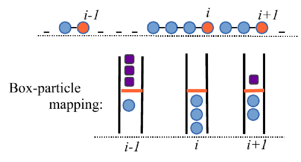
Along with this dynamics we also consider a reconstitution process among neighboring $k$-mers where one of the $k$-mers may release a single particle (or monomer) which instantly join the other $k$-mer. Reconstitution occurs at the interface of immobile $k$-mers which are expected to remain in contact for long time. That is, as described in Fig. 1, reconstitution process occurs among two $k$-mers $m$ and $m^{\prime}=m+1$ when they are in contact (so that $m$ is immobile) and when $m^{\prime}$ is blocked by another $k$-mer to its right (i.e. $m^{\prime}$ is also immobile):

$$(k_{m},~k_{n})\xrightleftharpoons[w(k_{n}+1,k_{m}-1)]{\,w(k_{m},k_{n})\,}(k_{m}-1,k_{n}+1).$$

(2)

The rate function $w(x,y)$ satisfy $w(1,y)=0,$ i.e., a $k$-mer can release the monomer only when its size is larger than unity. In other words, this restriction prohibits merging of $k$-mers, thereby keeping $M,$ the number of $k$-mers (and thus $\rho$ )conserved. It is evident that the dynamics Eqs. (1) and (2) also conserves $\rho_{0}.$

The dynamics of the model can be mapped exactly to a two-species generalization of misanthrope process by considering each $k$-mer as a box containing ${\kappa}=k-1$ particles of one kind ($k$-particles) and the number of consecutive vacancies say $n$ in front of the $k$-mer as the number of particles of other type ($0$-particles). This is described in Fig. 2. Thus in the box-particle picture, one of the constituting monomers of a $k$-mer (say the engine, marked as red in Fig. 2) is considered as the box containing two species of particles : additional monomer as one kind of particles (we refer to them as $k$-particles) and the vacancies in front of the $k$-mer as the other kind (referred here as $0$-particles). Thus, we have $M$ boxes containing $\tilde{K}=\sum_{m}^{M}{\kappa}_{m}=K-M$ number of $k$-particles and $N$ number of $0$-particles. Corresponding particle densities in the two-species misanthrope process (TMAP),

$\displaystyle\eta=\frac{K-M}{M}=\frac{1-\rho_{0}}{\rho}-1~~~~\text{and}~~~~\eta_{0}=\frac{N}{M}=\frac{\rho_{0}}{\rho}$

(3)

are conserved since they can be expressed in terms of conserved densities $\rho_{0}$ and $\rho$ defined on the lattice. Alternatively the densities $\eta_{0}$ and $\eta$ in TMAP uniquely fixes the densities on the lattice

$\displaystyle\rho_{0}=\frac{\eta_{0}}{1+\eta_{0}+\eta}~~~~~\rho=\frac{1}{1+\eta_{0}+\eta}.$

(5)

To illustrate the $k$-mer dynamics in the corresponding TMAP, a straightforward generalization of misanthrope process to two species, first let us define the dynamics explicitly. In TMAP, $0$- and $k$- particles hop out from a box $m,$ containing $(n_{m},{\kappa}_{m})$ number of $0$- and $k$-particles respectively to one of the neighboring boxes $m^{\prime}=m\pm 1$ having $(n_{m}^{\prime},{\kappa}_{m}^{\prime})$ particles with rates $u_{0}(n_{m},{\kappa}_{m};n_{m^{\prime}},{\kappa}_{m^{\prime}})$ and $u_{k}(n_{m},{\kappa}_{m};n_{m^{\prime}},{\kappa}_{m^{\prime}})$. Now, the dynamics of the reconstituting $k$-mers can be written as

	$\displaystyle u_{0}(n_{m},{\kappa}_{m};n_{m^{\prime}},{\kappa}_{m^{\prime}})$	$\displaystyle\equiv$	$\displaystyle\tilde{u}({\kappa}_{m})=u({\kappa}_{m}+1)\delta_{m^{\prime},m-1}$		(6)
	$\displaystyle u_{k}(n_{m},{\kappa}_{m};n_{m^{\prime}},{\kappa}_{m^{\prime}})$	$\displaystyle\equiv$	$\displaystyle\tilde{w}({\kappa}_{m},{\kappa}_{m^{\prime}})=w({\kappa}_{m}+1,{\kappa}_{m^{\prime}}+1)\delta_{n_{m},0}\delta_{n_{m^{\prime}},0},$		(7)

where the hop rate of $0$- particles $u({\kappa}_{m})$ does not depend on $n_{m},$ the number of particles of its own kind. The $\delta$-functions in the first equation forces $0$-particles to move towards left (same as $k$-mers moving to right) and those in the last equation takes care of the restrictions that reconstitution or monomer exchange occurs among neighboring boxes only when they are devoid of $0$-particles (equivalently, when $k$-mers are immobile).

The dynamics of $0$-particles is similar to that of a inhomogeneous ZRP [24] where hop rate of particles are different at different sites, but the background disorder here evolve continuously through reconstitution process. In fact a two species ZRP with one species following a dynamics similar to that of $0$-particles has been studied previously [25]. The dynamics of $k$-particles is however different here, and it is similar to the misanthrope process [26] where hop rate depends on both occupation number of departure and target boxes, but here we have additional interaction coming from the condition that both boxes must not contain $0$-particles during reconstitution. Thus we have an interacting TMAP where one species does misanthrope process in absence of the other species. The other species, on the other hand, hops in one direction with a inhomogeneous rate. Below we show that TMAP in this case evolves to a factorized steady state when $\tilde{w}(x,y)$ has a product form.

A product measure for TMAP would imply that the steady state probability of the system in a particular configuration can be written in the following form:

$$P\left(\{{\kappa}_{i},n_{i}\}\right)=\frac{1}{Q^{M}_{\tilde{K},N}}~~\prod_{i=1}^{M}f\left({\kappa}_{i},n_{i}\right)\delta\left(\sum_{i=1}^{M}{\kappa}_{i}-\tilde{K}\right)\delta\left(\sum_{i=1}^{M}n_{i}-N\right)$$

(8)

The $\delta$- functions introduced in the above equation ensures that the particle numbers $\tilde{K}$ and $N$ are conserved. Here, $f(\kappa,n)$ is some function yet to be determined in terms of the hop rates, and

$$Q_{\tilde{K},N}^{M}=\sum_{\{{\kappa}_{i}\},\{n_{i}\}}\prod_{i=1}^{M}f\left({\kappa}_{i},n_{i}\right)\delta\left(\sum_{i=1}^{M}{\kappa}_{i}-\tilde{K}\right)\delta\left(\sum_{i=1}^{M}n_{i}-N\right)$$

(9)

is the canonical partition function. It is clearly evident that the the steady state condition on the master equation can be satisfied if the $0$-particles satisfy a pairwise balance condition [27],

	$\displaystyle P(\{\dots,{\kappa}_{i}n_{i},{\kappa}_{i+1}n_{i+1},\dots\})\tilde{u}({\kappa}_{i+1})$		(10)
	$\displaystyle=P(\{\dots,{\kappa}_{i}n_{i}+1,{\kappa}_{i+1}n_{i+1}-1,\dots\})\tilde{u}({\kappa}_{i})$		(11)

and the $k$-particle hop rates satisfy a detailed balance condition

	$\displaystyle P(\{{\kappa}_{1}n_{1},\dots,{\kappa}_{i}0,{\kappa}_{i+1}0,\dots{\kappa}_{M}n_{M}\})\tilde{w}({\kappa}_{i},{\kappa}_{i+1})$		(12)
	$\displaystyle~~=P(\{{\kappa}_{1}n_{1},\dots,({\kappa}_{i}-1)0,({\kappa}_{i+1}+1)0,\dots{\kappa}_{M}n_{M}\})$		(13)
	$\displaystyle~~~~~~~~~~~~~~~~~~~~\times\tilde{w}({\kappa}_{i+1}+1,{\kappa}_{i}-1)$		(14)

These two equations along with the factorized steady state ansatz leads to

			$\displaystyle f({\kappa}_{i},n_{i})f({\kappa}_{i+1},n_{i+1})\tilde{u}({\kappa}_{i+1})$		(15)
			$\displaystyle~~~~=f\left({\kappa}_{i},n_{i}+1\right)f\left({\kappa}_{i+1},n_{i+1}-1\right)\tilde{u}({\kappa}_{i})$		(16)
	$\displaystyle{\rm and}~~$		$\displaystyle f({\kappa}_{i},0)f({\kappa}_{i+1},0)\tilde{w}({\kappa}_{i},{\kappa}_{i+1})$		(17)
			$\displaystyle~~~~=f({\kappa}_{i}-1,0)f(k_{i+1}+1,0)\tilde{w}({\kappa}_{i+1}+1,{\kappa}_{i}-1).$		(18)

Equation (16) is quite similar to the condition required to be satisfied in order to obtain factorized steady state in ZRP with site-dependent hop rate. Here, for any specific configuration, the profile of $\{{\kappa}_{i}\}$ of $k$-particles provide a inhomogeneous background on which $0$-particles hop. Although the background disorder evolve with time, we could obtain simple conditions ( Eqs. (16) and (18)) because the dynamics here restricts simultaneous hopping of $0$- and $k$-particles. We thus get the solution,

$$f({\kappa},n)=\left[\prod_{i=1}^{n}\frac{1}{\tilde{u}({\kappa})}\right]f({\kappa},0)=\left[\frac{1}{\tilde{u}({\kappa})}\right]^{n}f({\kappa},0),$$

(19)

where $f({\kappa},0)$ depends on the choice of the reconstitution rate $\tilde{w}.$ A factorized choice of rates $\tilde{w}({\kappa},{\kappa}^{\prime})=A({\kappa})B({\kappa}^{\prime})$ (when $f(0,0)$ is set to unity) gives,

$$f({\kappa},0)=\frac{B({\kappa}-1)}{A({\kappa})}f({\kappa}-1,0)=\left[\prod_{{\kappa}^{\prime}=1}^{\kappa}\frac{B({\kappa}^{\prime}-1)}{A({\kappa}^{\prime})}\right].$$

(20)

Using Eq. (19) we now get,

$\displaystyle f({\kappa},n)=u({\kappa})^{-n}\prod_{{\kappa}^{\prime}=1}^{\kappa}\frac{B({\kappa}^{\prime}-1)}{A({\kappa}^{\prime})}.$

(21)

Note that the functional form of $f({\kappa},0)$ in Eq. 20 is similar to what has been obtained for misanthrope process when the hop rate has a product form, $\tilde{w}({\kappa},{\kappa}^{\prime})=A({\kappa})B({\kappa}^{\prime})$ [26]. However, in this model, $k$-particles hop symmetrically in both directions (though with different rates) allowing us to frame a detailed balance condition which does not impose any further restrictions on the functional form of $A$ and $B.$ For directed hoping, the simplest possible balance condition is the pairwise balance, which restricts $A$ and $B$ to differ at best by a constant : $A(x)=B(x)-\alpha.$ We will study the model in presence of these restrictions in the following section and in Sec. IV we explore the possibility of phase separation transition when $A$ and $B$ are independent functions.

Our objective here is to investigate if reconstituting $k$-mers can undergo a phase separation transition in one dimension. This is equivalent to the possibility of having a condensation transition in TMAP. To this end we study the model in the grand canonical ensemble (GCE) and locate the regions in parameter space where macroscopic densities has a critical limit beyond which the densities cannot be controlled merely by tuning the fugacities. Therefore in these regions, a system having a conserved density larger than the critical limit is expected to produce a condensate carrying a finite fraction of particles in the system. Since there are two conserved densities, there could be four phases in general. In the TMAP the four distinct phases would correspond to condensation of either of the two species, or both or none of them.

The grand canonical partition function can be written for Eq. (9) as

$\displaystyle Z(x,z)$

$\displaystyle=$

$\displaystyle\sum_{N=0}^{\infty}\sum_{\tilde{K}=0}^{\infty}x^{\tilde{K}}z^{N}Q_{\tilde{K},N}^{M}=F(x,z)^{M},$

(22)

where

$\displaystyle F(x,z)=\sum_{{\kappa}=0}^{\infty}\sum_{n=0}^{\infty}x^{\kappa}z^{n}f({\kappa},n)=\sum_{{\kappa}=0}^{\infty}\frac{f({\kappa},0)x^{\kappa}}{1-z/\tilde{u}({\kappa})}$

(23)

and $x,z$ are the fugacities associated with $k$- and $0$-particles respectively. Corresponding densities are then,

$\displaystyle\eta(x,z)=\frac{x}{F}\frac{\partial F}{\partial x}~~{\rm and}~~\eta_{0}(x,z)=\frac{z}{F}\frac{\partial F}{\partial z}$

(24)

To proceed further we need to make a choice of $A({\kappa}),B({\kappa}^{\prime})$ and the drift rate $u({\kappa})$ which we do in the next section.

To illustrate the possible phase separation transitions in this model we chose a particular reconstitution rate

	$\displaystyle w({\kappa}+1,{\kappa}^{\prime}+1)=\tilde{w}({\kappa},{\kappa}^{\prime})=A({\kappa})B({\kappa}^{\prime})$		(25)
	$\displaystyle~~{\rm with}~~B({\kappa})=\frac{{\kappa}+2}{{\kappa}+1}~~{\rm and}~~A({\kappa})=\frac{{\kappa}+2}{{\kappa}+1}-\alpha$		(26)

that produces analytically tractable steady state solution. The parameter $0\leq\alpha\leq 1$ here controls the reconstitution rate. Note that in absence of $0$-particles (i.e., when the free volume $\rho_{0}=0$) the only dynamics in the system is reconstitution of $k$-mers. The dynamics of $k$-particles is similar to that of the misanthrope process [26] and thus we expect a condensation transition here.

For $\rho_{0}>0,$ the $k$-mers also drift towards right. Let us choose the drift rate as a step function

$$u(k)=\left\{\begin{array}[]{ll}v&{\rm for}~k\leq\mathbf{k}+1\cr~1&{\rm for}~k>\mathbf{k}+1\end{array}\right.$$

(27)

which has two free parameters $\mathbf{k}$ and $v.$ The $k$-mers having length smaller than a threshold $\mathbf{k}+1$ move to right with rate $v$ whereas others move with unit rate. In the box-particle picture, the corresponding hop rate $0$-particles is

$$\tilde{u}({\kappa})=\left\{\begin{array}[]{ll}v&{\rm for}~{\kappa}\leq\mathbf{k}\cr 1&{\rm otherwise}\end{array}\right.$$

(28)

Thus, the complete dynamics in the box-particle picture can be understood in the following way: $0$-particles hop to its right on a inhomogeneous background which itself evolves with time as $k$-particles also hop symmetrically following a misanthrope process (26). In this case (up to a constant factor),

$\displaystyle f({\kappa},0)=\frac{{\kappa}!}{(c)_{\kappa}}({\kappa}+1)^{2},~{\rm with}~~c=\frac{3-2\alpha}{1-\alpha}$

(29)

where $(c)_{\kappa}=c(c+1)\cdots(c+{\kappa}-1)$ the Pochhammer symbol. Thus the partition function in the GCE, following Eqs. (22) and (23), is $Z(z,x)=F(x,z)^{M},$ with

	$\displaystyle F(x,z)=\frac{z(1-v)G_{\mathbf{k}}(x)+(v-z)G_{\infty}(x)}{(1-z)(v-z)}$		(30)
	$\displaystyle{\rm where}~G_{\mathbf{k}}(x)=\sum_{{\kappa}=0}^{\mathbf{k}}\frac{{\kappa}!}{(c)_{\kappa}}({\kappa}+1)^{2}x^{\kappa}.$		(31)

It is evident that the maximum value of the fugacity $z$ is $z_{c}=min\{1,v\}$ and that of $x$ is $x_{c}=1.$ Corresponding densities are then,

	$\displaystyle\eta_{0}(x,z)$	$\displaystyle=$	$\displaystyle\frac{z}{1-z}+\frac{zv(1-v)G_{\mathbf{k}}(x)}{(v-z)[z(1-v)G_{\mathbf{k}}(x)+(v-z)G_{\infty}(x)]}$		(32)
	$\displaystyle\eta(x,z)$	$\displaystyle=$	$\displaystyle x\frac{z(1-v)G_{\mathbf{k}}^{\prime}(x)+(v-z)G^{\prime}_{\infty}(x)}{z(1-v)G_{\mathbf{k}}(x)+(v-z)G_{\infty}(x)}.$		(33)

controlled by $0<x<x_{c}$ and $0<z<z_{c}.$ Here ^′ indicates derivative with respect to $x.$ Since both the densities are increasing functions of $x$ and $z$, the maximum achievable macroscopic density lies along the lines $x=x_{c}$ and $z=z_{c}.$ Thus we can have four different phases (A) the fluid phase ($x<x_{c}$ and $z<z_{c}$) (B) $k$- particle condensate ($z<z_{c}$ and $x=x_{c}$) (C) $0$-particle condensate ($z=z_{c}$ and $x<x_{c}$)and (D) condensation of both ($x=x_{c}$ and $z=z_{c}$).

One interesting scenario is $z=0$ where $\eta_{0}=0$ and $\eta(x,0)=xG^{\prime}_{\infty}(x)/G_{\infty}(x)$ which in the limit $x\to 1$ gives $\eta^{c}=4/(c-5).$ This is same as a misanthrope process with rates given by Eq. (26) $-$ accordingly the partition function is given by $G_{\infty}(x)^{M}.$ In the lattice model, however the free volume is $\rho_{0}=0$ and $k$-mer number density beyond which the condensation transition occurs is $\rho^{c}=1/(1+\eta^{c})=(c-5)/(c-1).$ This transition is different from the usual phase separation transitions observed in lattice models. Here the free volume being zero, the only dynamics is the reconstitution process which produces one macroscopically large $k$-mer in the pool of other $k$-mers of much smaller sizes.

Another interesting limit is $z\to z_{c}.$ In this case, $\eta_{0}$ in Eq. (33) diverges (as the first-term in r.h.s diverges when $v>1$ and the second term when $v<1$) which results in $\rho_{0}=\eta_{0}/(1+\eta_{0}+\eta)\to 1.$ Thus, the critical value density for $\rho_{0}=1$ is $\rho^{c}=0.$ In other words, when the $k$-mer number density is very low, they always form a condensate irrespective of the value of $v.$

We proceed further with $\mathbf{k}=2$ and $c=7$ to demonstrate the possibility of phase separation. In this case monomers ($k=1$ or ${\kappa}=0$), dimers (${\kappa}=1$) and trimers (${\kappa}=2$) move with rate $v$ whereas other $k$-mers move with rate $1.$ Calculations for non-integer $c$ or $\mathbf{k}>2$ are straight forward and generate long expressions involving Hypergeometric functions, but it does not provide any additional physical insight. Now, the densities can be calculated from Eq. (33) by using

	$\displaystyle G_{\infty}(x)$	$\displaystyle=$	$\displaystyle\frac{30}{x^{6}}(5-x)(1-x)^{3}Log(1-x)+\frac{5}{2x^{5}}(2-x)(30-66x+37x^{2});$		(34)
	$\displaystyle G_{2}(x)$	$\displaystyle=$	$\displaystyle 1(16x+9x^{2})/28$		(35)

Each point in $x$-$z$ plane corresponds to unique densities ($\eta_{0},\eta$). To obtain the extremal limits of these densities we plot variation of $\eta_{0}$ as a function $\eta$ for different contour lines in $x$-$z$ plane which approach to either $x=x_{c}=1$ or to $z=z_{c}=1$. Figure 3(a) demonstrates, for $v=2$, how $\eta_{0}$ varies with $\eta$ when the fugacity $x$ approaches its critical limit $x_{c}$ following the the contours $x_{c}-x=0.1,0.01$ and $0.001$ (denoted as solid lines $c,b,a$). Similarly the contours of $z_{c}-z=0.1,.01,0.001$ and corresponding density variations in $\eta$-$\eta_{0}$ plane are shown as dashed lines $d,e,f$. It is evident that when $z$ approaches its critical value $z_{c}=1$ and $0\leq x\leq x_{c},$ the lines in $\eta$-$\eta_{0}$ plane diverges. However, for the other limit $x\to 1$ (with $0\leq z\leq 1$) the contour lines in $\eta$-$\eta_{0}$ plane reaches a limiting curve and thus densities beyond this line (shown as shaded region) cannot be achieved in the GCE by tuning the fugacities $x$ and $z.$ The equation of this limiting or critical line, $x=1$ , can be translated to $\eta$-$\eta_{0}$ plane by expressing $\eta_{0}^{c}\equiv\eta_{0}(1,z)$ as a function of $\eta^{c}\equiv\eta(1,z)$ (red lines in Fig. 3(a) and (b)).

Thus the density conserving dynamics, given by Eqs. (26) and (27), cannot distribute particles macroscopically if densities $(\eta,\eta_{0})$ lie in this region. But what would be the background density ?

In a recent work [28], Großkinsky proposed a procedure to obtain the background density from the grand canonical distributions. It was argued that the normal directions of the critical line in $\mu_{x}$-$\mu_{z}$ plane (here chemical potentials are $\mu_{x}=\ln(x)$ and $\mu_{z}=\ln(z)$) translates to a direction in density plane along which the background density remain invariant. For TMAP, the critical line is $x=1$ (i.e. $\mu_{x}=0$) and thus the normals are defined by $z=constant.$ For illustration, we take $z=0.8$ in Fig. 3(b) and plot the corresponding contour in $\eta$-$\eta 0$ plane (shown as dashed line). It approaches to the critical point $Q\equiv(\eta^{c},\eta_{0}^{c})$ with a slope given by the tangent line PQR. The Großkinsky criteria indicate that the background density along the line QR in the condensate phase is invariant and is given by the critical point Q. Clearly, for any arbitrary density $(\eta,\eta_{0})$ on the line QR, $\eta>\eta^{c}$ and $\eta_{0}>\eta^{c}_{0}$; both species would have extra particles which would form a condensate. Such lines, drawn in Fig. 3(b) for other values of $z$ clearly indicate that both $k$ - and $0$- particles condensate in phase D.

For generic values of $v>0$ the densities $(\eta,\eta_{0})$ are finite along the line $x=1$ and the critical line $x=1$ translates to,

	$\displaystyle\eta^{c}$	$\displaystyle=$	$\displaystyle 2\frac{(53+17v)z-70v}{(53v+17)z-70v}~~~~~or~~~~z=\frac{70v(\eta^{c}-2)}{17(\eta_{c}-2v)+53(\eta^{c}v-2)}$		(36)
	$\displaystyle\eta_{0}^{c}$	$\displaystyle=$	$\displaystyle\frac{z}{1-z}+\frac{v}{v-z}+\frac{70v}{(17+53v)z-70v}$		(37)
		$\displaystyle=$	$\displaystyle\frac{(2-\eta^{c})\{17v(53\eta^{c}-34)^{2}+53(17\eta^{c}-106)^{2}\}}{72(v-1)(53\eta^{c}-34)(17\eta^{c}-106)}$		(38)

The critical lines for the condensation transition in TMAP are shown in Fig. 4(a) for different values of $v.$ In the inset we show the $k$-particle condensate phase (shaded region) for for $v=1/2$ and $v=2.$

Note that for $v<1$ the condensate phase is of type B where only $k$-particle condensate. Unlike $v>1$ case, here $0$- particles hop out faster from the sites with large $k$ values (particularly the condensate site) inhibiting formation of condensation. Again, for $v=1,$ all $k$-mers drift with equal rate, and thus the reconstitution dynamics become identical to a misanthrope process of $k$-particles, forming a condensate for $\eta>\eta_{c}=4/(c-5)=2.$ Also, for $\eta_{0}=0$ the condensation always occurs at $\eta=2$ independent of $v$ as in this case there is no free volume available for drift. The critical lines can be explained in the following way: for $0<v\leq 1$ the possible values of $\eta^{c}$ lies in the range $0<\eta^{c}\leq 2.$ However from Eq. (38) we have a divergence of $\eta_{0}^{c}$ at $\eta^{c}=34/53$. Thus the critical line for $v<1$ is obtained by choosing the accessible values for $\eta^{c}$ in the range $34/53<\eta^{c}<2$ and obtaining the corresponding values for $\eta_{0}^{c}$ from Eq. (38). Similarly, to ensure positivity and finiteness in $\eta_{0}^{c},$ the critical line for $v>1$ must be bounded in the region $2<\eta^{c}<106/17$. Note that when $\eta_{0}$ is increased, the transition occurs for lower $\eta$ values when $v<1$, i.e., when monomers, dimers and trimers move slower than other $k$-mers. Naturally, this scenario reverses for $v>1.$ It is also evident that for $\eta>106/17$ condensation occurs for any $\eta_{0}>0.$

To observe the phase separation transition, we finally translate these transition lines in $\eta$ -$\eta_{0}$ plane to $\rho_{0}$-$\rho$ plane in Fig. 4(b) using Eq. (5). $\eta_{0}^{c}$ in Eq. (38) diverges in this limit. In Fig. 4(b), the phase separated state is shown as shaded region , for $v=1/2$ and $v=2.$

In the previous section we have observed only some of the condensate phases where due to reconstitution, one of the $k$-mers may become macroscopically large and $0$-particles are attracted to the condensate site when it moves with a slower rate. It is however possible to have an independent condensation of vacancies as they experience an evolving disordered background: slow moving $k$-mers may accumulate macroscopic number of vacant sites in front of it forming an additional condensate phase. To study all these possible scenarios we choose a hop rates having a single parameter $b>0$ as

$$A({\kappa})={\kappa}+b,~~B({\kappa})={\kappa}+1~{\rm and}~\tilde{u}({\kappa})=\frac{{\kappa}+2}{{\kappa}+1}.$$

(39)

In this case $f({\kappa},0)={\kappa}!/(1+b)_{\kappa}$ and thus

$$f({\kappa},n)=\frac{{\kappa}!}{(1+b)_{\kappa}}\left(\frac{{\kappa}+1}{{\kappa}+2}\right)^{n}$$

(40)

Note that the weight factor $f({\kappa},0)$ is same as what one gets for an ordinary ZRP [29] with particle hop rate $u_{{}_{ZRP}}(k)=1+b/k$ (even though $k$-particles here follow a misanthrope dynamics). Thus, in absence of $0$-particles it is assured that a condensation transition occurs for large densities when $b\geq 2.$ In absence of $k$-particles , however, $0$-particles follow a simple ZRP dynamics with a constant rate $\tilde{u}(0)=2$ and they cannot form a condensate. We proceed to see that the interaction between $0$- and $k$-particles can provide an additional phase where only $0$-particles condensate.

A model with steady state weight given by Eq. (40) has been studied in context of two-species ZRP [25] which exhibit all possible condensate phases depending on the value of $b$ [25, 28]. For completeness we revisit the model for $b=4$ where all different condensate phases are present; we then translate the transition lines to obtain the phase separation scenario in driven $k$-mer models in one dimension.

In GCE the partition function is $Z(x,z)=F(x,z)^{M}$. Following Eq. (23) we get

	$\displaystyle F(x,z)$	$\displaystyle=$	$\displaystyle\left[36x^{4}(2z-1)(3z-2)\right]^{-1}~[~x^{2}(19xz-14x+42z-30)$		(41)
		$\displaystyle-$	$\displaystyle 6\ln(1-x)\left\{x(3z-2)(2zx^{2}-x^{2}-3)+2(2z-1)\right\}$		(42)
		$\displaystyle-$	$\displaystyle 12(2z-1)-36x^{4}(1-z)^{2}\Phi\left(x,1,(2-z)/(1-z)\right)~]$		(43)

where $\Phi(.,.,.)$ is the Lerch Phi function, and factors which are independent of $x$ and $z$ are ignored. The corresponding densities can now be obtained using Eq. (24). We avoid writing down those long expressions explicitly. Instead, in the following, we focus on the results only at the critical limits. It is evident that $F(x,z)$ diverges as $x\to x_{c}=1$ (logarithmically) and for $z\to z_{c}=1$.

As long as the equivalence of grand canonical and canonical ensemble holds i.e., in the density regions bounded by the parametric curves $\{\eta(x,z_{c}),\eta_{0}(x,z_{c})\}$ and $\{\eta(x_{c},z),\eta_{0}(x_{c},z)\}$ in the $\eta-\eta_{0}$ plane, the system remains in the fluid-phase. Condensation occurs when these parametric functions become finite valued $-$ then in the canonical ensemble, densities larger than these values does not have any representative fugacities, thus resulting in condensation. For $b=4$ we have the critical lines,

$$\eta(x,1)=\frac{x(11x^{2}+30x-48)-6\ln(1-x)(8-9x+x^{3})}{x(12-12x-5x^{2})+6\ln(1-x)(2-3x+x^{3})}$$

(44)

$$\eta_{0}(x,1)=1+\eta(x,1)$$

(45)

$$\eta(1,z)=h(z)\left[74-67z-36(2-z)(1-z)H_{\frac{1}{1-z}}\right]$$

(46)

	$\displaystyle\eta_{0}(1,z)$	$\displaystyle=$	$\displaystyle 6zh(z)\left[6\psi_{1}\left(\frac{2-z}{1-z}\right)\right.$		(48)
			$\displaystyle+\left.\frac{64z-37z^{2}-25+6(1-z)(3-5z)\{\gamma+\psi_{0}\left(\frac{2-z}{1-z}\right)\}}{(3z-2)(2z-1)}\right]$

where $h(z)=[36(1-z)^{2}H_{\frac{1}{1-z}}+37z-32]^{-1}$ with $H_{m}$ being the Harmonic number, $\psi_{m}(.)$ is the poly-gamma function of order $m$ and $\gamma$ is the Euler constant.

In Fig. 5 (a) we have plotted these parametric functions $\eta_{0}$ versus $\eta,$ for $x=x_{c}$ varying $0<z<1$ (blue curve) and then for $z=z_{c}$ varying $0<x<1$ (red curve). These two critical lines encapsulate a region where macroscopic density is well described by the fugacities $x$ and $z$ (denoted by A, the fluid phase). To investigate the possibility of condensation in the other density regions, we follow the Großkinsky criteria [28] described in the previous section. In fact, the phase diagram for a different model having the same steady state structure has been explored in details [28]. The $k$-condensate occurs in the region beyond $x=x_{c}$ curve (denoted by B), whereas $0$-particles condensate in the density region above $z=z_{c}$ curve in $\eta$-$\eta_{0}$ plane (denoted as C). Finally the density region $D$ corresponds to condensation of both kind of particles. The transition lines in box-particle picture are then translated to the $k$-mer densities on the lattice using Eq. (5). Correspondingly, the $k$-mers show three different kind of phase separated states along with the fluid phase A, as shown in Fig. 5(b). Note that, the fluid phase here corresponds to a phase where $k$-mers are well mixed with the vacancies. This requires small free volume $\rho_{0}\approx 1$ and large $k$-mer number density $\rho$ so that size of each $k$-mer is small.

To demonstrate the four-phase scenario, we simulate the drifting reconstituting $k$-mer dynamics on a system of size $L=900$. Starting from a random initial distribution of $k$-mers the system is allowed to evolve for $10^{5}$ MCS; for the next $10^{3}$ MCS, we store the location and size of $k$-mers and color them as follows, $k$-mer: blue, engine: red and vacancy: orange. Figure 6 (A) (B) (C) and (D) shows the space-time (downwards) plot of these configurations for four different points $(\eta,\eta_{0})=(1/4,1/4),(2,1),(1/2,5/2)$ and $(2,5)$, representing four different phases respectively. All three different condensate phases show striking co-existence features whereas the fluid phase is well mixed. Note that $k$-particles show a localized condensate as reconstitution (or $k$-particle hop in TMAP) occurs symmetrically, whereas the $0$-condensate moves towards left.

In this article we study the possibility of phase separation transition in a one dimensional system of poly-dispersed hard extended objects called $k$-mers which occupy $k$ consecutive lattice sites. A $k$-mer can move by one lattice site with a rate $u(k)$ which depends on its size, if the rightward neighbor is vacant. Along with the drift, $k$-mers also undergo reconstitution, where two consecutive $k$-mers of size $k$ and $k^{\prime}$, if immobile due to hardcore constraint (i.e., their immediate right neighbor are not vacant) can exchange one particle between them with rate $w(k,k^{\prime})$; thus their sizes become either $(k-1,k^{\prime}+1)$ or $(k+1,k^{\prime}-1).$ This dynamics conserves the total volume occupied by the $k$-mers. We also impose an additional conservation of the number of $k$-mers by restricting $w(k,k^{\prime})=0$ for $k<2$. We find that this additional conservation can lead to four distinct phases : (A) a fluid phase where similar size $k$-mers are well mixed with the vacancies, (B) one macroscopic $k$-mer and rest of the system remaining homogeneous, (C) a very slow moving $k$-mer leaving a trail of vacancies (macroscopic void) in front of it, and (D) a macroscopic void along with a macroscopic $k$-mer.

We could obtain the exact boundaries which separate four different phases by mapping the model to a two-species misanthrope process (TMAP) by considering $k$-mers as boxes containing $k-1$ particles of one kind (called $k$-particles) and the number of vacancies in front of it as particles of other type (called $0$-particles). The effective dynamics in TMAP becomes the following: $k$-particles in boxes which are devoid of $0$- particles evolve following the dynamics of a misanthrope process with rate $w(k-1,k^{\prime}-1)$ and the $0$-particles hop with a inhomogeneous rate that depend on the number of $k$-particles present in the box. The interplay of interaction between two different species is now evident. $k$- particles hop only when both departure and arrival boxes are devoid of $0$-particles, and $0$-particle hop rate depends on the number of $k$-particles.

We must mention that in ZRP and related models with one or more species, if a dynamics involving asymmetric hopping of particles (say, only to rightward neighbour) evolve to a factorized steady state, then the model also shares the same steady state if particle hopping were symmetric. In the model that we have studied, in the presence of directional drive, reconstitution occurs when two $k$-mers are (a) in contact, and (b) the right $k$-mer has no empty site to its right. In fact, condition (b) naturally decouples the dynamics of $0$ and $k$-particles and help in obtaining an explicit factorized steady state. When $k$-mers drift only towards right, the condition (b) can be interpreted as follows: only immobile $k$-mers (which are more likely to remain in contact) can exchange particle among them. In case of symmetric diffusion of $k$-particle, such an interpretation would be lost in $k$-mer picture, but the steady state however is not altered. To model a more realistic situation like dynamics of polymerization [30] or filaments in micro channels [31], we need to extend this dynamics to higher dimensions and to include a fusion dynamics which breaks the conservation of number of $k$-mers and a fragmentation dynamics which allow breaking of a $k$-mer into two random segments.

Acknowledgments: We thank the anonymous referee for his valuable comments and constructive suggestions. BD gratefully acknowledges the financial support of Council of Scientific Research, India (Ref. 09/489(0089)/2011-EMR-I). PKM gratefully acknowledges the support of CEFIPRA under Project 4604-3.

References

- [1] B. Schmittmann and R. K. P. Zia, Statistical Mechanics of Driven Diffusive Systems, Phase Transitions and Critical Phenomena, Vol. 17, ed. by C. Domb, J. L. Lebowitz (Academic Press, 1995).
- [2] D. Mukamel, Soft and Fragile Matter: Nonequilibrium Dynamics, Metastability and Flow, edited by M.E. Cates, M.R. Evans (Institute of Physics Publishing, Bristol, 2000).
- [3] M. R. Evans, Y. Kafri, H. M. Koduvely, and D. Mukamel, Phys. Rev. Lett. 80, 425 (1998); M. R. Evans, Y. Kafri, H. M. Koduvely, and D. Mukamel, Phys. Rev. E 58, 2764 (1998)
- [4] R. Lahiri and S. Ramaswamy, Phys. Rev. Lett. 79, 1150 (1997); R. Lahiri, M. Barma, and S. Ramaswamy, Phys. Rev. E 61, 1648 (2000).
- [5] Y. Kafri, E. Levine, D. Mukamel, G.M. Schütz, and R.D.W. Willmann, Phys. Rev. E 68 035101 (2003); M. R. Evans, E. Levine, P. K. Mohanty, and D. Mukamel, Eur. Phys. J. B 41, 223(2004).
- [6] Y. Kafri, E. Levine, D. Mukamel, G. M. Schütz, and J. Török Phys. Rev. Lett. 89, 035702 (2002).
- [7] P. F. Arndt, T. Heinzel, and V. Rittenberg, J. Phys. A 31, L45(1998); P. F. Arndt, T. Heinzel, and V. Rittenberg, J. Stat.Phys. 97, 1 (1999).
- [8] L. Tonks, Phys. Rev. 50, 955 (1936).
- [9] C. T. MacDonald, J. H. Gibbs, and A. C. Pipkin, Biopolymers 6, 11 (1968); C. T. MacDonald and J. H. Gibbs, Biopolymers 7, 707 (1969).
- [10] T. Sasamoto and M. Wadati, J. Phys. A: Math. Gen. 31, 6057 (1998).
- [11] L. B. Shaw, R. K. P. Zia, and K. H. Lee, Phys. Rev. E 68, 021910 (2003).
- [12] G. Schönherr and G. M. Schütz, J. Phys. A: Math. Gen. 37, 8215 (2004).
- [13] L. B. Shaw, A. B. Kolomeisky, and K. H. Lee, J. Phys.A: Math. Gen. 37, 2105 (2004).
- [14] L. B. Shaw, J. P. Sethna, and K. H. Lee, Phys. Rev. E 70, 021901 (2004).
- [15] J. J. Dong, B. Schmittmann, and R. K. P. Zia, Phys. Rev. E 76, 051113 (2007).
- [16] S. Gupta, M. Barma, U. Basu, and P. K. Mohanty, Phys. Rev. E 84, 041102 (2011).
- [17] Z. W. Salsburg, R. W. Zwanzig, and J. G. Kirkwood, J. Chem. Phys. 21, 1098 (1953).
- [18] G. I. Menon, M. Barma, and D. Dhar, J. Stat. Phys. 86, 1237 (1997).
- [19] D. Dhar, Physica A 315, 5 (2002).
- [20] M. Barma, M. D. Grynberg, and R. B. Stinchcombe, J. Phys.:Condens. Matter 19, 065112 (2007);
- [21] M. D. Grynberg, Phys. Rev. E 84, 061145 (2011).
- [22] A. Rákos and G.M. Schütz, J. Stat. Phys. 118, 511 (2005).
- [23] F. Spitzer, Adv. in Math. 5, 246 (1970).
- [24] C. Godréche and J. M. Luck, J. Stat. Mech.: Theory Exp. P12013 (2012).
- [25] T. Hanney and M. R. Evans, Phys. Rev. E 69, 016107 (͑2004); S. Großkinsky and T. Hanney, Phys. Rev. E 72, 016129 (2005).
- [26] M. R. Evans and B. Waclaw, J. Phys. A, Math. Theor.47, 095001 (2013).
- [27] G. M. Schütz, R. Ramaswamy and M. Barma, J. Phys. A: Math. Gen. 29, 837 (1996).
- [28] S. Großkinsky, Stoch. Proc. Appl. 118, 1322 (2008) .
- [29] M. R. Evans and T. Hanney, J. Phys. A: Math. Gen., 36 L441 (2003) ; ibid, J. Phys. A: Math. Gen. 38, R195 (2005).
- [30] S. M. Yu. et. al., Nature 389, 167 (1997); A. L. Martin et. al., FEBS Lett. 480, 116 (2000); L. Edelstein-Khshet and G. B. Ermentrout, J. Math. Biol. 40, 64 (2000).
- [31] S. K’́oster, D. Steinhauser and T. Pfohl, J. Phys.: Cond. Mat. 17, S4091 (2005).