Compressibility enhancement in an almost staggered interacting Harper model

The interplay between electron-electron (e-e) interactions and quasi-disorder has drawn much excitement since the discovery of quasi-crystals [1, 2]. Much of the work has focused on a specific model of a one-dimensional (1D) quasi-crystal, namely the Harper (or Aubry-André) model [3, 4]. One of the main attractions of this model is that contrary to conventional 1D disordered systems which are localized for any amount of disorder [5], the Harper model exhibits a metal-insulator transition as function of the quasi-disordered potential strength, even in the absence of interactions [4, 6, 7, 8, 9, 10, 11]. The influence of e-e interactions on the metal-insulator transition of the Harper model was studied in several publications [12, 13, 14]. Interest in the Harper model has lately peaked after it has been shown that for an irrational modulation, the Harper model may be a 1D topologically nontrivial system, and have topological boundary states  [15, 16, 17, 18, 19, 20, 21, 22, 23]. This property, coupled with the fact that the Harper model may be realized in the context of cold atoms and molecules [24, 25] added to the excitement surrounding the Harper model.

Recently, an additional aspect of the model has been investigated, namely the inverse compressibility, which measures the change in the chemical potential when an electron is added to the system. In the context of disordered quantum dots this has become a very popular measurement to extract information on the role of e-e interactions in these systems [26, 27, 28]. For a finite system of $N$ particles, $\Delta_{2}(N)$, is defined as the change in the chemical potential due to the insertion of the $N^{\rm th}$ particle i.e., $\Delta_{2}(N)=\mu(N)-\mu(N-1)$, where $\mu(N)$ is the chemical potential for $N$ particles. Since $\mu(N)=\mathcal{E}(N)-\mathcal{E}(N-1)$ (where $\mathcal{E}(N)$ is the system’s many-body ground-state energy with $N$ particles), $\Delta_{2}(N)$ is given by:

For non-interacting systems at zero temperature,

where $E_{N}$ is the $N^{\rm th}$ single-particle eigenenergy and $\Delta(N)$ is the single-particle level spacing.

How do the e-e interactions affect the inverse compressibility? The conventional wisdom leads to the constant interaction (CI) model [28, 29], which essentially assumes that the interactions between the electrons are well described by mean-field. This leads to the conclusion that the effect of interactions on the inverse participation given by $\Delta_{2}(N)=\Delta(N)+e^{2}/C$, where $C$ is the total classical capacitance. Thus, the e-e interactions increase the inverse compressibility compared to its non-interacting value. This description fits well the experimental measurements in quantum dots [28].

However, the CI mean-field description doesn’t hold at certain conditions. It has been shown [30, 31, 32] that close to the Mott metal-insulator transition occurring at half-filling of a clean the Hubbard model, the inverse compressibility may decreases with the Hubbard interactions strength. Recently, it has been shown [33] that for the almost staggered Harper model of spinless electrons with nearest-neighbors e-e interactions, close to half-filling, the system becomes more compressible as the interactions are increased, although no metal-insulator transition occurs there. This counter intuitive behavior stems from the properties of the electronic bands and density for the almost staggered Harper model. Under these conditions the non-interacting Harper model has an almost flat narrow band around zero energy, separated from the other bands by large gaps. The density of the narrow band around half-filling is anti-correlated with the on-site potential, whereas the density of the lower occupied bands follows the potential. Therefore, once e-e interaction is introduced, the electrons in the lower occupied bands squeeze out the states in the narrow central band, resulting in a narrower central band. This flattening of the central band due to the interaction with the lower band electronic density results in an increase of the compressibility.

In this paper we address the question whether this increase of the compressibility is the result of the particular model studied in Ref. [33]. Specifically, we shall see what happens to the compressibility when the spin degree of freedom is taken into account, or equivalently when considering a spinless two legged ladder. Another case which we explore is when next nearest neighbors interactions are included. To study the compressibility we mainly rely on the HF approximation, which has been shown to be extremely accurate for this model [33] due to the large gap between the flat central band and the lower band and to the localized nature of the states in the narrow band. We will also compare some of these results to density matrix renormalization group (DMRG) numerical calculations, which for these 1D systems are essentially exact [34, 35], and describe very well the dependence of the ground state energy on the number of particles [36]. Using DMRG we also show that the enhancement of the compressiblity is accompanied by the suppression of the entanglement entropy.

In this section we discuss the influence of the spin degree of freedom on the compressibility in the staggered Harper model close to half-filling. The clearest difference between spin-polarized (spinless) and non-polarized electron is the fact that for non-polarized (spinfull) electrons there are Hubbard interactions. The on-site potential is spatially modulated with a frequency of almost two lattice-sites period (i.e., staggered), corresponding to fast modulation with a slow envelope. The interaction terms are repulsive and short ranged (on-site and nearest-neighbors (n.n.)-interactions). We assume that in the limit of weak Hubbard interactions no spin polarization occurs, i.e., the total $S_{z}=0$ for even filling and $S_{z}=\pm 1/2$ for odd filling. We show that the compressibility of the system decrease when the Hubbard interactions are increased by analyzing the central (flat) energy band close to half-filling. Due to the Kramers degeneracy, as long as there is no spin flip (tunneling between the ladders’ legs), the single-particle solution is just a duplication of the spinless solution presented in Ref. [33]. Thus, it contains two copies of superlattice states that reside at the valleys of the potential envelope. Since the electrons are localized in the potential valleys, adding an additional electron to a valley will increase the energy due to the Hubbard interaction. In order to reduce the effect of the Hubbard interaction the electronic density must rearrange itself. As a result, the capacitance of the system goes down.

In order to demonstrate that behavior we need to explicitly solve the tight-binding Harper model for fermions with spin and with Hubbard and n.n. repulsive interactions given by:

where $c_{j,s}$ is the single particle annihilation operator at site $j$ with spin $s$ and $n_{j,s}=c^{\dagger}_{j,s}c_{j,s}$ is the number operator. $t,t^{\prime}\in\mathbb{R}$ are the site hopping and spin flipping amplitudes, respectively. $\lambda>0$ controls the on-site potential amplitude. The potential is a cosine modulated in space with frequency $b$ and a phase factor $\phi$ . $U>0$ and $U^{\prime}>0$ are the strengthens of the repulsive n.n. and Hubbard interactions, respectively. We discuss the region $\lambda<2t$, which is the metallic regime [4]. We further assume that $b\mod 1=1/2+\epsilon$, $\epsilon\ll 1/2$ corresponding to an almost staggered case. $\epsilon\in\mathbb{R}$ is non-rational so that the system is disordered.

Let us first discuss the non-interacting Hamiltonian, i.e., set $U,U^{\prime}=0$ in Eq. (3). A numerical solution in this case reveals the existence of an almost flat central energy band (see Fig. 1), splitted due to the spin flip matrix element to a lower and higher central band. We are mostly interested in the central band energy spectrum, and since these energy states which are close to zero minimize both kinetic and potential energy, we conclude that the most important contribution comes from states localized in the potential valleys, i.e. states localized around the position $l_{z}$ corresponding to $2\pi\epsilon l_{z}+\phi=(\mathbb{Z}+\frac{1}{2})\pi$ [33]. In the valley, we can approximate $\cos(2\pi\epsilon j+\phi)\approx 2\pi|\epsilon|(j-l_{z})s_{z}$, and $s_{z}=-sign(\sin(2\pi\epsilon l_{z}+\phi))=\pm 1$. The effective Hamiltonian describing the central band is

where

is the sub-lattice pseudo-spinor that splits the lattice into even and odd sites, according to $c_{ek,s}=\frac{2}{L}\sum_{j=1}^{L/2}e^{ik2j}c_{2j,s}$ and $c_{ok,s}=\frac{2}{L}\sum_{j=1}^{L/2}e^{ik(2j-1)}c_{2j-1,s}$. $\hat{p}_{k}\equiv i\partial_{k}$ and $\sigma_{x},\sigma_{z}$ are the $2\times 2$ Pauli matrices.

Diagonalizing the spin degrees of freedom (which are independent of k-space), we get

This representation allows us to write the Hamiltonian as a sum of two distinct subspaces, each relates to a different spin eigenstate. The subspaces depend only on the momentum $k$, and therefore can be solved using the same methods used for spinless fermions [33]. Thus, the eigenenergies for the Hamiltonian of the potential valleys are $E_{1}^{val}=\pm\sqrt{8n}\dfrac{t}{\xi}+t^{\prime}$, and $E_{2}^{val}=\pm\sqrt{8m}\dfrac{t}{\xi}-t^{\prime}$, where $m,n\in\{0,1,2...\}$, and $\xi^{2}=\dfrac{t}{\pi\lambda|\epsilon|}$. $E_{1}^{val},E_{2}^{val}$ correspond to the spin states $1,2$ respectively. The central zero-energy band splits due to the spin flip, resulting in an energy splitting between the two bands equal to $2t^{\prime}$.

The eigenfunctions for the states belonging to the splitted central band are:

where $|j,i>=\frac{1}{\sqrt{2}}(c_{j,\uparrow}^{\dagger}\pm c_{j,\downarrow}^{\dagger})|\emptyset>$ , where $|\emptyset>$ is the vacuum state. These wavefunctions are Gaussians of width $\xi$ around $l_{z}$. In the limit of small $t^{\prime}$ our assumptions hold and this result is a good approximation of the real ground state.

These states form a basis for the central band, defined by $m,n=0$, since $<l_{z,i}|l_{z\pm 1,i}>=0,<l_{z,1}|l_{z,2}>=0$, and $|<l_{z,i}|l_{z^{\prime},i}>|\leq e^{-\frac{(l_{z}-l_{z^{\prime}})^{2}}{2\xi^{2}}}\ll 1$.

Let us now consider the contribution of the overlap between the localized states in the central band. The Gaussian decay of the localized states implies that the Hamiltonian matrix elements, $<l_{z,i}|H|l_{z^{\prime},j}>$, are not negligible only between nearest neighbors states $|z-z^{\prime}|=1$. Thus, the central band states follow an effective Hamiltonian:

Diagonalizing this Hamiltonian yields the eigenstates

with eigenvalues $E^{central}(k)=-2\bar{t}\cos(k)\pm t^{\prime}$.

Now, let us focus on the case where the Hubbard interactions in the Hamiltonian Eq. (3) are turned on ($U^{\prime}\neq 0$), but no longer range interactions are yet considered ($U=0$). For $U^{\prime}\rightarrow\infty$ the model can be solved analytically. In that limit only the interaction term is important. The eigenenergies are therefore $E=0$ and $E=U^{\prime}$. The latter case occurs when two particles with opposite spins occupy the same site. This will cost infinite energy and therefore such states are decoupled from the theory. The remaining states contain a single particle per site.

Next, we consider the case where $U^{\prime}$ is much bigger than the other energy scales in the theory, i.e. $U^{\prime}\gg t,t^{\prime},\lambda$. Using perturbation theory with $t$ as the perturbation parameter on the Hubbard model reveals that ferromagnetism is the lowest energy state. Adding $t^{\prime}$ to the theory will not change the ground state, since the correction in $t^{\prime}$ will be of at least third order in perturbation theory.

As is discussed in Ref. 33, because the central band is essentially protected by the large gaps to the other bands, the HF approximation results are very accurate. Therefore, we approximate the Hubbard interaction using the HF method for interaction strength values smaller than these gaps $U^{\prime}\ll\sqrt{8}\dfrac{t}{\xi}$.

Rewriting the Hamiltonian in Eq. (3) with $U=0$, and ignoring the constant term which is simply a shift in the energy, results in

We find that the averaged electronic density between the valleys of potential is $<n_{j,s}>\approx\frac{1}{4}-\frac{1}{2}(-1)^{j}\bar{n}(\frac{\lambda}{2t})\cos(2\pi\epsilon j+\phi))$ , with $\bar{n}(x)=\dfrac{x}{\pi\sqrt{1+x^{2}}}K(\frac{1}{1+x^{2}})$, and $K$ is the complete elliptical integral of the first kind. Hence

where $\lambda_{eff}=\lambda-U^{\prime}\bar{n}(\dfrac{\lambda}{2t})$.

The solutions of $H^{HF}$ are closely related to the solutions of $H$ in the non-interacting case. Yet, the width of the valley states, $\xi$, has changed due to the change in $\lambda$.

Moreover, for n.n.-interactions ($U\neq 0$) it is possible to use the HF approximation, and obtain the HF eigenstates and eigenvalues, which are identical to the non-interacting solutions, up to the modified parameters $\tilde{t}$, and $\tilde{\lambda}$ [33]. The many-body density and the exchange terms are proportional to those obtained already for the spinless case [33] up to a proportionality constant of $1/2$, due to the spin degrees of freedom. Therefore, $<p_{j,s}>\approx\frac{1}{2}\bar{p}(\frac{\lambda}{2t}\cos(2\pi\epsilon j+\phi))$. Between the potential valleys this can be approximated by $<p_{j,s}>\approx\frac{1}{2}\bar{p}(\frac{\lambda}{2t})$.

We can now write the HF. Hamiltonian with both Hubbard and n.n. interactions:

with $t_{eff}=t+\frac{1}{2}U\bar{p}(\frac{\lambda}{2t})$ and $\lambda_{eff}=\lambda+(2U-U^{\prime})\bar{n}(\dfrac{\lambda}{2t})$.

We again can solve the system with the modified parameters, and obtain the HF eigenvalues and eigenstates,

where the Gaussian decay parameter $\xi=\xi(\frac{t_{eff}}{\lambda_{eff}})$ is modified due to the effective values taken by $\lambda$ and $t$. $\xi^{2}$ is multiplied by a numerical constant equal to $1.16$ as in [33].

Projecting the HF Hamiltonian on the central band yields

The eigenvalues and the eigenstates of the central band are then given by:

with $L_{z}=\lfloor 2|\epsilon|L\rfloor$ the number of valley states. The hopping amplitude $\bar{t}^{HF}$ is given by

Thus the inverse compressibility $\Delta_{2}(N)$ can be calculated using (2) and the eigenvalues are presented in Eq. (14).

As shown in Fig. 2, $\Delta_{2}(N)$ decreases with the n.n.-interaction $U$, in agreement with the case of spinless fermions [33]. However, the Hubbard interaction $U^{\prime}$ enhances $\Delta_{2}(N)$. As was shown in Eq. (10), the Hubbard interaction reduces the value of the effective Harper potential amplitude, $\lambda_{eff}$. The decrease in $\lambda_{eff}$ increase the width of the Gaussian wavefunctions. Thus, there is more overlap between different states and therefore any change of configuration in the system, such as adding another particle, requires more energy. For $U=2U^{\prime}$ the system returns to the non-interacting Hamiltonian value of $\Delta_{2}(N)$. The interplay between $U$ and $U^{\prime}$ determines weather $\Delta_{2}(N)$ will be larger ($U<2U^{\prime}$) than its non-interacting value or smaller ($U>2U^{\prime}$) than it.

For an intuitive understanding let us revisit Fig. 1. The states which occupy the lowest energy band reside in the valleys of potential. When the Hubbard interaction is turned on, occupying these states become too costly in energy for some of the spins. In order to avoid the Hubbard interaction they tend to occupy the surroundings of potential peaks, where there are less spins to interact with. This tendency delocalizes the Gaussian wavefunctions. However, since only half of the particles participate in the interaction between the opposite spins it is less significant (by a factor of $\frac{1}{2}$) than $U$.

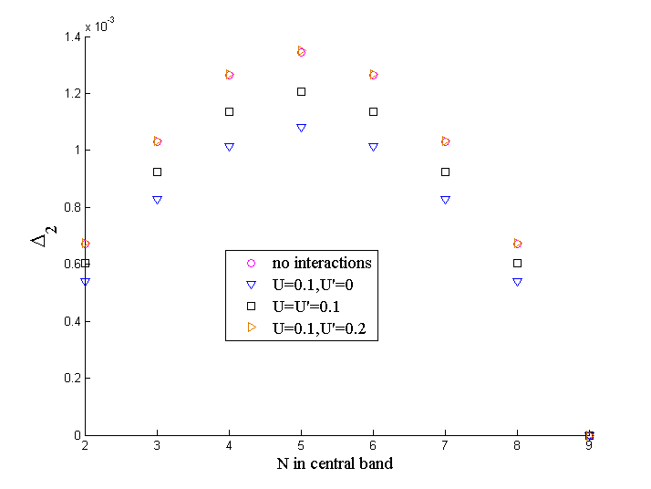
An exception to this behavior is found for the state at edge of the lower splitted band. As detailed earlier, due to the spin flipping amplitude $t^{\prime}$, a gap of size $2t^{\prime}$ opens between the lower central band occupied by $\frac{1}{\sqrt{2}}(\uparrow+\downarrow)$ states and the higher central band with states corresponding to $\frac{1}{\sqrt{2}}(\uparrow-\downarrow)$ . $\Delta_{2}(N)$ decreases with $U^{\prime}$ and increases with $U$ at the edge, similar to the behavior observed close to the half-filling point of the 1D Hubbard model [30].

In order to understand the behavior of the compressibility for a system with long range interactions, we consider here the influence of next nearest neighbors interaction. For simplicity, we discuss spinless fermions. The results of this section can be easily extended for fermions with spin using the methods described in the previous section.

The Hamiltonian is given by:

and the mean-field approximation yields

where $<n_{j}>$ is the (already known) background density. The background exchange energy is $<\tilde{p_{j}}>\equiv<c_{j}^{\dagger}c_{j+2}>$. Here we ignore constant terms, since they do not contribute to $\Delta_{2}$. Using the known value of $<n_{j}>|_{\epsilon=0}$,

Interestingly, the exchange term disappears (the calculation appears in the appendix) resulting in

This structural robustness can be attributed to the symmetry of the non-interacting Hamiltonian’s wavefunctions used in the calculation. Thus, the additional interaction only changes the value of $\lambda_{\rm eff}$ without changing the structure of the HF Hamiltonian. The effective Hamiltonian becomes

where $\bar{t}^{HF}$ given by Eq. (15) with $t_{eff}=t+\frac{1}{2}U\bar{p}(\frac{\lambda}{2t})$ and $\lambda_{eff}=\lambda+(2U-2U_{2})\bar{n}(\dfrac{\lambda}{2t})$. Here we ignored on-site terms, which just lead to an over all energy shift.

We also calculate $\Delta_{2}(N)$ using DMRG [34, 35], for the following parameters: $b=\sqrt{30}$ (corresponding to $\epsilon\approx-0.023$) and $\phi=0.7\pi$. The length of the system is $L=200$, and we calculated the ground state energy $\mathcal{E}(N)$ for each number of electrons $N=91,92,\ldots,108$. For $t=1$, the potential amplitude was chosen as $\lambda=0.7$, which results in a flat central band, with the typical $\Delta_{2}$ greater than the numerical accuracy. Interaction strengths of $U=0$, $U_{2}=0$ and $U=0.1$ with $U_{2}=0,0.025,0.05,0.075$ are considered. The boundary conditions are open, since it significantly improves accuracy [34] and we retain $384$ target states. The accuracy of $\Delta_{2}$ is about $\pm 1\cdot 10^{-4}t$ and the discarded weight is $\sim 10^{-7}$.

The resulting change in the compressibility can be viewed in Fig. 3. Comparing the analytic values to the results obtained using the numerical DMRG results, we find good agreement between the two methods. Here the Gaussian decay parameter $\xi^{2}$ is modified according to $\xi^{2}\rightarrow 1.16\xi^{2}(1-0.4U_{2})$. The $1.16$ factor arise from using the linear approximation of the potential also between the valleys, leading to a too-fast decay of the wave function as was discussed for the n.n interactions [33]. For the n.n. interaction an additional linear dependence of $\xi$ on $U_{2}$ is needed. It seems that the longer-range interaction results in an additional correction of the wave function behavior in the valleys.

With the additional interactions the compressibility ($1/\Delta_{2}$) decreases. Intuitively, the increase in the value of $\lambda$ due to the interaction results a decrease in the Gaussian decay parameter $\xi^{2}$, which results in a greater overlap between the wavefunctions. This can be interpreted as a change in the local nature of the system due to the next n.n.-interactions which delocalizes the wavefunctions. Thus, adding another particle costs more energy. This additional energy cost is reflected in the growth of $\Delta_{2}(N)$.

The opposite behavior between the n.n and next n.n. interactions can also be observed in the behavior of the bipartite entanglement entropy. The entanglement entropy of a system in a pure state $|\Psi\rangle$ is defined as the von Neumann entropy of the reduced density matrix of region A, $\hat{\rho}_{A}={\rm Tr}_{B}|\Psi\rangle\langle\Psi|$, where the degrees of freedom of the rest of the system (region B) are traced out, resulting in

For the 1D Harper model the system is divided between regions A and B, where region A is of length $L_{A}$ while region B is the remaining $L-L_{A}$ sites.

The entanglement entropy for a typical state in the central band is depicted in Fig. 4. The behavior of $S_{A}$ is non-monotonous, quite different than the entanglement entropy of a clean wire, and has several intriguing features. Here we will concentrate on the feature directly pertaining to the compressibility. The most obvious feature are the peaks appearing in $S_{A}(L_{A})$. It is apparent that the positions of the peaks not immediately adjacent to the edges correspond to the positions of the central band states $|l_{z,i}>$. These peaks are very robust and do not change when the interaction strength is changed. On the other hand, the entanglement of the minimum between the peaks are influenced by the interactions. When n.n. interactions ($U$) are introduced the entanglement in the minimum regions are suppressed (this is clearly seen in the enlarge segment in Fig. 4). When next n.n. interactions ($U_{2}$) are added, the entanglement minimum remains closer to its non-interacting value. This follows exactly the pattern exhibited by the inverse compressibility ($\Delta_{2}(N)$) is reduced. One can speculate that the entanglement is related to the extension of the band state $|l_{z,i}>$ into its nearest neighbor, and thus the suppression of $\Delta_{2}(N)$ is related to the suppression of the entanglement. It is interesting whether it might be possible to directly relate the compressibility to the entanglement in a similar manner to the relation between fluctuations in the number of particles and entanglement [37]. This is left for further study.

In this paper we considered the variation of the inverse compressibility $\Delta_{2}(N)$ with respect to repulsive Hubbard interaction and next n.n.-interaction in the central band of the almost staggered fermionic Harper model in the vicinity of half-filling. The behavior of the central band states is studied using the HF approximation, justified by the flatness of this band and its isolation from the other bands. For the next n.n.-interaction we also calculated $\Delta_{2}(N)$ using DMRG. The comparison between the two methods promise reliable results. We found both for the Hubbard interaction and for the next n.n. interactions an increase in $\Delta_{2}(N)$, which corresponds to a decrease in the compressibility of the system. Thus, the increase in the compressibility due to the n.n. interactions is somewhat suppressed once Hubbard or next n.n. interactions are considered. It is interesting to note the different role played by the Hubbard interactions for the clean 1D Hubbard model and the Harper model. For the clean Hubbard model close to to the metal-insulator phase transition at half-filling of 1D systems, the Hubbard interaction enhance compressibility [30]. This behavior is also manifested for the Harper model close to the edge of the lower central band. On the other hand, for the rest of the central band, the Hubbard term effectively reduces the strength of the on-site potential in the system ($\lambda_{eff}<\lambda$) and thus the energy gaps become smaller, weakening the enhancement of compressibility. Open questions, such as the classification of interaction terms (which terms lead to delocalization and decrease in $\Delta_{2}(N)$, and which localize the wavefunctions and increase $\Delta_{2}(N)$) and the full understanding of the non monotonous entanglement entropy, remain for further study.

For the Hamiltonian with $U=\epsilon=0$, the energy spectrum of the central band is $E_{k,\pm}=\pm\sqrt{4t^{2}\cos^{2}(k)+\lambda^{2}\cos^{2}\phi}$. The corresponding eigenstates are

where

The exchange energy is given by $<\chi_{k,\pm}|c^{\dagger}_{j+2}c_{j}|\chi_{k,\pm}>=e^{-2ik}(\chi_{ek,\pm}^{2}+\chi_{ok,\pm}^{2})$.

Normalization yields

$\chi_{ek,\pm}^{2}+\chi_{ok,\pm}^{2}=1$.

Assuming the lower band is fully occupied,

$<c^{\dagger}_{j+2}c_{j}>|_{\epsilon=0}=\int^{\pi/2}_{-\pi/2}\dfrac{dk}{\pi}<\chi_{k,-}|c^{\dagger}_{j+2}c_{j}|\chi_{k,-}>=0$.

References

- [1] D. Shechtman, I. Blech, D. Gratias, and J. W. Cahn, Phys. Rev. Lett. 53, 1951 (1984).
- [2] D. Levine, and P. J. Steinhardt, Phys. Rev. Lett. 53, 2477 (1984).
- [3] P. G. Harper, Proc. Phys. Soc. London A 68, 874 (1955).
- [4] S. Aubry and G. André, Ann. Isr. Phys. Soc. 3, 133 (1980).
- [5] P.A. Lee and T.V. Ramakrishnan, Rev. Mod. Phys. 57, 287 (1985).
- [6] For a review see H. Hiramoto and M. Kohmoto, Int. J. Mod. Phys. B 6, 281 (1992).
- [7] S. Ya. Jitomirskaya, Annals of Mathematics 150, 1159 (1999).
- [8] G. Roati, C. D’Errico, L. Fallani, M. Fattori, C. Fort, M. Zaccanti, G. Modugno, M. Modugno and M. Inguscio, Nature 453, 895 (2008).
- [9] Y. Lahini, R. Pugatch, F. Pozzi, M. Sorel, R. Morandotti, N. Davidson, Y. Silberberg, Phys. Rev. Lett. 103, 013901 (2009).
- [10] J. Chabé, G. Lemarié, B. Grémaud, D. Delande, P. Szriftgiser, J. C. Garreau, Phys. Rev. Lett. 101, 255702 (2008).
- [11] G. Modugno, Rep. Prog. Phys. 73, 102401 (2010).
- [12] J. Vidal, D. Mouhanna, and T. Giamarchi, Phys. Rev. Lett. 83, 3908 (1999); Phys. Rev. B 65, 014201 (2001).
- [13] C. Schuster, R. A. Römer, and M. Schreiber Phys. Rev. B 65, 115114 (2002) .
- [14] S. Iyer, V. Oganesyan, G. Refael, and D. A. Huse Phys. Rev. B 87, 134202 (2013).
- [15] Y. E. Kraus, Y. Lahini, Z. Ringel, M. Verbin, and O. Zilberberg, Phys. Rev. Lett. 109, 106402 (2012).
- [16] Y. E. Kraus and O. Zilberberg, Phys. Rev. Lett. 109, 116404 (2012).
- [17] K. A. Madsen, E. J. Bergholtz, and P. W. Brouwer Phys. Rev. B 88, 125118 (2013).
- [18] M. Verbin, O. Zilberberg, Y. E. Kraus, Y. Lahini, and Y. Silberberg, Phys. Rev. Lett. 110, 076403 (2013).
- [19] Z. Xu, L. Li, and S. Chen, Phys. Rev. Lett. 110, 215301 (2013).
- [20] S. Ganeshan, K. Sun, and S. Das Sarma, Phys. Rev. Lett. 110, 180403 (2013).
- [21] F. Grusdt, M. Höning, and M. Fleischhauer, Phys. Rev. Lett. 110, 260405 (2013).
- [22] Z. Xu and S. Chen, Phys. Rev. B 88, 045110 (2013).
- [23] I. I. Satija and G. G. Naumis, Phys. Rev. B 88, 054204 (2013).
- [24] M. Aidelsburger, M. Atala, M. Lohse, J. T. Barreiro, B. Paredes, and I. Bloch, Phys. Rev. Lett. 111, 185301 (2013).
- [25] H. Miyake, G. A. Siviloglou, C. J. Kennedy, W. C. Burton, and W. Ketterle, Phys. Rev. Lett. 111, 185302 (2013).
- [26] U. Sivan, R. Berkovits, Y. Aloni, O. Prus, A. Auerbach, and G. Ben-Yoseph Phys. Rev. Lett. 77, 1123 (1996).
- [27] R. Berkovits, Phys. Rev. Lett. 81, 2128 (1998).
- [28] Y. Alhassid, Rev. Mod. Phys., 72, 895 (2000).
- [29] I. L. Kurland, I. L. Aleiner, and B. L. Altshuler, Phys. Rev. B 62, 14886 (2000).
- [30] T. Usuki,N. Kawakami, A. Okiji, Phys. Lett. 135A, 476 (1989).
- [31] N. Furukawa, M. Imada, J. Phys. Soc. Jpn. 61, 3331 (1992).
- [32] F. F. Assaad, M. Imada, Phys. Rev. Lett. 76, 3176 (1996).
- [33] Y. E. Kraus, O. Zilberberg and R. Berkovits, Phys. Rev. B 89, 161106(R) (2014).
- [34] S. R. White, Phys. Rev. Lett. 69, 2863 (1992); Phys. Rev. B48, 10345 (1993).
- [35] U. Schollwöck, Rev. Mod. Phys. 77, 259 (2005); K. A. Hallberg, Adv. Phys. 55, 477 (2006).
- [36] R. Berkovits, F. von Oppen, and Y. Gefen Phys. Rev. Lett. 94, 076802 (2005).
- [37] H. F. Song, S. Rachel, C. Flindt, I. Klich, N. Laflorencie, and K. Le Hur, Phys. Rev. B 85, 035409 (2012).