Optimal Sparse Output Feedback Controller Design:
A Rank Constrained Optimization Approach
Abstract
We consider the problem of optimal sparse output feedback controller synthesis for continuous linear time invariant systems when the feedback gain is static and subject to specified structural constraints. Introducing an additional term penalizing the number of non-zero entries of the feedback gain into the optimization cost function, we show that this inherently non-convex problem can be equivalently cast as a rank constrained optimization, hence, it is an NP-hard problem. We further exploit our rank constrained approach to define a structured output feedback control feasibility test with global convergence property, then, obtain upper/lower bounds for the optimal cost of the sparse output feedback control problem. Moreover, we show that our problem reformulation allows us to incorporate additional implementation constraints, such as norm bounds on the control inputs or system output, by assimilating them into the rank constraint. We propose to utilize a version of the Alternating Direction Method of Multipliers (ADMM) as an efficient method to sub-optimally solve the equivalent rank constrained problem. As a special case, we study the problem of designing the sparsest stabilizing output feedback controller, and show that it is, in fact, a structured matrix recovery problem where the matrix of interest is simultaneously sparse and low rank. Furthermore, we show that this matrix recovery problem can be equivalently cast in the form of a canonical and well-studied rank minimization problem. We finally illustrate performance of our proposed methodology using numerical examples.
I INTRODUCTION
The problem of optimal linear quadratic controller design has been extensively studied for several decades. In conventional control, it is usually assumed that all measurements are accessible to a centralized controller, while in large scale interconnected systems this assumption is not practical, since it is often desirable that subsystems only communicate with a few neighboring components due to the high cost and, sometimes, infeasibility of communication links. Therefore, the need to exploit a particular controller structure, obtained based on the layout of the system network, seems undeniable. Furthermore, the traditional controller synthesis methods, which are closely related to solving the Algebraic Riccati Equation, no longer work when additional constraints are imposed on the structure of the controller.
In general, the problem of designing constant gain feedback controllers subject to additional constraints is NP-hard [1]. In recent years, numerous attempts have been made to provide distributed controller synthesis approaches for different classes of systems [2, 3, 4, 5, 6]. Bamieh et al, in [7, 8], investigated the distributed control of spatially invariant systems, then the work in [9] has proved that the solution of Riccati and Lyapunov equations for systems consisting of Spatially Decaying (SD) operators has SD property, which lends credibility to the search for controllers that have access only to local measurements. The design of optimal state feedback gain in the presence of an a priori specified structure, usually in the form of sparsity patterns, is considered in [5]. In their recent papers, Lavaei et al. [10, 11, 12] cast the problem of optimal decentralized control for discrete time systems as a rank constrained optimization problem, developed results on the possible rank of the resulting feasible set, and introduced several rank-reducing heuristics as well. Wang et al. studied the problem of localized LQR/LQG control and presented a synthesis algorithm for large-scale localizable systems [13, 14]. Frequency domain approaches to design optimal decentralized controllers are also presented in [15, 16, 17].
In the design of linear feedback controllers for interconnected systems, a common desired structure is that the controller matrices are sparse, which could correspond to a simpler controller topology and fewer sensors/actuators. However, fewer measurement/communication links leads to performance deterioration and sometimes even instability of the overall system. Therefore, there exists a trade off between the stability and performance of the system and minimizing the number of non-zero entries of the feedback gain matrices. The problem of minimizing the number of nonzero elements of a vector/matrix subject to a set of constraints in inherently NP-hard and arises in many fields, such as Compressive Sensing (CS) where the inherent sparseness of signals is exploited in determining them from relatively few measurements [18]. Since the advent of Compressive Sensing, considerable work has been done on the design of compressive measurement matrices based on different criteria such as sparse signal support detection and estimation [19, 20], sparse signal detection and classification [21, 22], etc.
To alleviate the issues caused by the combinatorial nature of cardinality functions, several convex/non-convex functions have been proposed as surrogates for the cardinality functions in optimization problems. For example, in cases where the optimization constraint is affine, -norm , as a convex relaxation of -norm, has proved to work reliably under certain conditions, namely Restricted Isometry Property (RIP) [23, 24, 25]. Thus, -norm and its weighted versions have been extensively used in signal processing and control applications [26, 27, 28]. Non-convex relaxations of the cardinality function, such as -quasi-norm (), have also received considerable attention recently [29, 30]. In [31, 32, 33], it is shown that, for a large class of SD systems, the quadratically-optimal feedback controllers inherit spatial decay property from the dynamics of the underlying system. Moreover, the authors have proposed a method, based on new notions of -Banach algebras, by which sparsity and spatial localization features of the same class can be studied when is chosen sufficiently small.
In the present paper, we consider the problem of optimal sparse feedback controller synthesis for linear time invariant system, in which convex constraints are imposed on the structure of the controller feedback gain. The main contribution of our paper is to propose a novel approach which allows us to equivalently represent the intrinsically nonlinear constraints, such as closed loop stability condition and enforcement of controller structure, with a single rank constraint in an otherwise convex optimization program. Having all non-linearities encapsulated in only one rank constraint allows us to employ one of several existing algorithms to efficiently solve the resulting problem.
Our results are distinct from those reported in [26], as we present an alternative formulation which not only solves the regular sparse controller design problem, but also enables us to solve the output feedback control problem. Furthermore, integrating various types of nonlinear system constraints, such as constraints on the controller matrix and its norms, into the existing rank constraint can be effortlessly implemented in our approach. It should also be noted that the rank constraint emerging in our approach originates from the positive definiteness of the Lyapunov matrix and the properties of fixed rank matrices, thus the ratio of matrix dimension and its rank does not grow with the size of system. In contrast, the rank one constraint appears in [12] results from utilizing the auxiliary variable introduced by self multiplying the vector formed by augmenting the states, inputs, and outputs, hence there exist a linear growth of the ratio of the dimension of the matrix to its rank as the number of variable increases, which is a computational drawback in controller synthesis for large scale systems.
We start by augmenting the -norm of the feedback gain matrix to the quadratic cost function of our optimization problem. This additional term penalizes the extra communication links in the feedback pathway. We then reformulate it into an equivalent optimization problem where the non-convex constraints are lumped into a rank constraint. Based on the notions of holdable ellipsoid, we propose a reformulation of the problem to incorporate norm bounds on the control inputs and outputs of the system, which usually appear in controller implementations. Employing a convex relaxation of the added cardinality term, based on the weighted -norm, we argue that Alternating Direction Method of Multipliers (ADMM) is well-suited to solve our problem, since our search is to obtain a solution with an a priori known rank. ADMM iteratively solves the rank-unconstrained problem and projects the solution into the space of the matrices with the desired rank until the convergence criteria are met. We further investigate the special case of designing the sparsest stabilizing controller, and show that this problem can be rewritten as a rank minimization problem. Rank minimization problems have received considerable attention in recent years [34, 35, 36]. In [37], it is shown that if a certain Restricted Isometry Property holds for the linear transformation defining the constraints, the minimum rank solution can be recovered by solving the minimization of the nuclear norm over the feasible space. Therefore, the nuclear norm may be used as a proxy for the rank minimization in our problem.
The remainder of this paper is organized as follows. In Section II, the general optimal sparse output feedback control problem setup is defined. Section III, we reformulate the optimal sparse output feedback control problem as a rank constrained problem, and develop several results based on the proposed reformulation. In Section IV, we study the convex relaxation of this problem, and discuss the application of ADMM in solving the problem. The special case where the sparsity penalizing factor dominates the quadratic terms in the cost function is described in Section V. Numerical examples illustrating the proposed methods are provided in VI. Finally, Section VII concludes the paper.
Notations: Throughout the paper, the following notations are adopted. The space of by matrices with real entries is indicated by . The by identity matrix is denoted . Operators and denote the trace and rank of the matrix operands. The transpose and vectorization operators are denoted by and , respectively. The Hadamard product is represented by . A matrix is said to be Hurwitz if all its eigenvalues lie in the open left half of the complex plane. represents the cardinality of a vector/matrix, while and denote and Frobenius norm operators.Also, the norm is defined by
A real symmetric matrix is said to be positive definite (semi-definite) if all its eigenvalues are positive (non-negative). () denotes the space of positive definite (positive semi-definite) real symmetric matrices, and the notation () means ().
II Problem Formulation
Let a linear time invariant system be given by its state space realization
where is the state vector, is the output of the system, is the control input, and matrices , and have appropriate dimensions. We consider designing a constant gain output feedback stabilizing controller
| (3) |
with the minimum number of non-zero entries that minimizes a quadratic objective function. We further assume that the set of all acceptable a priori specified structures for feedback gains, denoted by , is a convex set. The reason behind this call is that such an assumption not only reduces the complexity of the problem, but also convex constraints on controller constraints have broad real-world applications. For example, there exist numerous applications in which establishing a link between two particular nodes is impractical either due to physical constraints or extremely high costs; such limitations can be incorporated into the design process by imposing the convex constraints that the corresponding entry of the controller gain should be zero. Also, other regularly occurring limitations such as upper bounds on the entries of the controller matrix can be also be implemented by convex constraints on matrix .
In addition, we consider an upper bound on the norm of the control input and the closed loop system output . The search for such a controller can be formulated as an optimization problem, in which the sparsity of the feedback gain is incorporated by adding the -norm of the gain matrix to the objective function. The -norm denotes the cardinality of the feedback gain, hence, it penalizes the number of non-zero entries of the matrix. Therefore, we have the following optimization problem
| (P1) | ||||
| s.t. | ||||
where and are performance weight matrices, is the initial state, and is the regularization parameter. Also, the value of in the norm can be either infinity or two. It is possible to rewrite our main optimization problem in the following equivalent form [38].
| (4) | ||||
| s.t. | ||||
| Hurwitz, | ||||
The feedback gain matrix derived from solving the above optimization problem depends on the value of the initial state . To avoid re-solving the minimization problem for every value of , we design a state feedback controller which minimizes the expected value of the cost function assuming that the entries of are independent Gaussian random variables with zero mean and covariance matrix equal to the positive definite matrix , i.e. . Using Lyapunov stability theorem, it can be easily checked that the global asymptotic stability of the closed loop system is guaranteed if and only if the matrix is positive definite, thus we can rewrite the optimization problem as follows
| (5a) | ||||
| s.t. | (5b) | |||
| (5c) | ||||
| (5d) | ||||
| (5e) | ||||
| (5f) | ||||
where , , and . In optimization problem (5), the constraints (5b-5d) are convex, nevertheless, the constraints (5e) are nonlinear and the control input/output constraints (5f) are in time domain, hence, the problem is non-convex.
III Rank Constrained Formulation
In traditional LQR problems, with no input/output constraints, the nonlinear constraints can be replaced by a linear matrix inequality to form an equivalent convex problem. However, the addition of the sparsity penalizing term to the cost function, the existence of structural constraints on the feedback gain matrix, and incorporation of input/output bounds differentiate our problem from the conventional LQR problem, making the conventional approach inapplicable. Here, we propose a controller synthesis approach based on the idea that the non-convex constraints can be replaced by a rank constraint. Before proceeding, lets state the following lemma.
Lemma III.1.
Let , , , and , with . Then, if and only if and , where
Proof.
Since , its inverse exists and the matrix can be decomposed as
where
Since the matrices pre/post-multiplied by the matrix are full rank, the matrix is rank if and only if the rank of the matrix is , which is equivalent to
This completes the proof of the lemma. ∎
The following corollary is now immediate.
Corollary III.2.
Assuming , the constraint
is equivalent to
For legibility purposes, we first develop the equivalent formulation for the case with no constraint imposed on the control inputs/outputs, then, we incorporate the bounds on the input/output of the closed loop system.
III-A Rank Constraint Formulation with no Input/Output Constraint
Assuming that no upper bound is defined for the input/output of the controlled system, the next proposition states that the nonlinear Semidefinite Program (5) can be cast as an optimization problem, where all constraints are convex except one, which is a rank constraint.
Proposition III.3.
Proof.
Applying Lemma III.1 to the constraints and , they can be equivalently replaced by the rank constraint
since is constrained to be positive definite. Introducing the auxiliary matrix variable , we can employ Corollary III.2 to rewrite the above rank constraint as a rank constraint on a symmetric matrix, i.e. . ∎
It should be noted that augmenting the matrix to the original rank constrained matrix only adds some redundant constraints along with an extra variable. Although we increase the number of variables by introducing the new n-by-n variable , having a symmetric rank constrained matrix has proved to be helpful, as we aim to use a positive semidefinite relaxation of the rank constraint later in this paper, thus, it is crucial to associate the rank constraint to a symmetric matrix.
Remark III.4.
The optimal value of in problem (P2) is the inverse of the optimal , i. e. .
III-B Feasibility of the output feedback control problem
Before proceeding with the addition of the input/output constraints to the problem formulation, we discuss how our proposed rank constrained reformulation can be exploited in investigating the feasibility of the output feedback control problem under constraints such controller pre-defined structure and input/output constraint. We further utilize the proposed formulation to obtain the upper/lower bounds for the optimal cost of the optimal sparse output feedback control problem. Although the results in this section are stated for the case where no input/output bound is enforced on the controller, they can be effortlessly extended to incorporate such constraints. The next theorem introduces a feasibility test for the existence of a stabilizing output feedback controller with predefined structure.
Theorem III.5.
Proof.
Applying the results from [39, p.266], if the matrix is positive semidefinite, i.e. , we have
| s.t. | |||
where are the eigenvalues of . Due to positive semidefiniteness of , the optimal cost of (6) is lower bounded by zero. Now, using our rank constraint formulation, it can be verified that such an output feedback controller, satisfying the predefined structure, stabilizes the LTI system (II) if and only if the feasible set of (6) contains at least a matrix with rank for which the sum of smaller eigenvalues is equal to zero, i.e. . ∎
The optimization problem (6) is non-convex due to the existence of the the bi-linear term in its cost function. However, it can be solved utilizing a globally convergent optimization algorithm, which iteratively solves the problem for and till it reaches the convergence [40, 41].
Next, we investigate the bounds on the optimal cost of the optimization problem P2. Assuming feasibility, the lower bound for the optimal cost can be evidently achieved by relaxing the rank constraint by the positive semidefinite constraint , since the PSD constraint defines a super-set for the set determined by the rank constraint. As a result, the feasible set of the rank constraint optimization P2 is a subset of the feasible set of the relaxed problem, hence, the optimal cost of the relaxed optimization provides us with a lower bound for original problem. A more detailed discussion is provided in Section IV-A.
As for the upper bound, the results of the theorem III.6 can be utilized to obtain such a bound if either there is no pre-defined structure on the controller gain or the set of the acceptable controller structures, i.e. is assumed to be invariant with respect to positive scaling. This assumption covers the highly applicatory structural constraint, where the feasibility/infeasibility of feedback paths are a priori specified generally through a directed graph representation. In such cases the feedback link can be established only if its corresponding edge of the graph, i.e. the pair of vertices and edges respectively, is existent, as shown in equation (7).
| (7) |
Theorem III.6.
Assuming the set is invariant under positive scaling, the optimal cost of the following optimization problem provides an upper bound for the solution of the rank constrained problem (P2).
| (8) | ||||
| s.t. | ||||
where
Proof.
The proof is similar to that of the theorem III.7; hence, omitted. ∎
Next, we state another version of the previous theorem which is valid when the state feedback controller design is intended. Due to the simpler structure of this problem, a tighter upper bound can be achieved by employing the following theorem.
Theorem III.7.
Assuming the set is invariant under positive scaling, the optimal cost of the following optimization problem provides an upper bound for the solution of the rank constrained problem (P2) in the case of feedback controller synthesis, i.e. .
| (9) | ||||
| s.t. | ||||
where
Proof.
First, we show that the following optimization problem solves the optimal state feedback control problem, i.e. (P2) with .
| (10) | ||||
| s.t. | ||||
where
Scaling the last block-row and column of the matrix in (P2), assuming the scaler is not zero, does not affect the rank constraint, thus we can equivalently rewrite it as
The -norm is invariant under positive scaling, hence . Also, Since the set is assumed to be invariant under positive scaling, the constraint is identical to the matrix belonging to the set of admissible controller structures. Therefore, it is possible to rewrite the optimization problem in terms of the new variable, defined as .
In optimization problem (10), due to the positive definiteness of , the constraint is equivalent to positive definiteness of its Schur complement, that is
which holds if and only if , i.e. , and , where . Therefore, the feasible set of (P2) is a subset of the feasible set of (10). To conclude our proof, it suffices to show that the optimal value of in the optimization problem (10) is zero.
Lets assume is the optimal solution to (10), where is not zero. The optimal cost corresponding to this optimum, namely , becomes
Since , setting , along with the same values of , , and , also belonging to the feasible set, generates a lower cost. This contradicts the optimality of , hence the optimal value of must be zero. Therefore, the optimization problem (10) solves the problem (P2) when .
III-C Rank Constraint Formulation in Presence of Input/Output Constraints
Next, we present how an upper bound on the norm of the control input/output can be incorporated into our rank constrained formulation. It is known that for the positive scaler satisfying , where is the initial state of the system and is the solution to the Lyapunov stability condition, the set
| (11) |
is an invariant set for the closed loop system. Employing the concept of invariant sets for linear systems, we can develop the rank constraint formulation of control system with bounded input norms. The details for two choices of norms utilize to bound the control input in given in the sequel.
- •
System Norm: The next theorem describes how the upper bound on the system norm of the control input can be incorporated into the controller synthesis problem using our proposed rank constrained formulation.
Theorem III.8.
The optimization problem (P2) can be modified to conservatively incorporate an upper bound on the system norm of the control input, i.e. , as follows.
(P3) s.t. where denotes the initial state and
Proof.
Based on the lines in [42, p. 103], we have
Thus, the input constraint holds for all if
The existence of the term in the above matrix inequality makes it nonlinear, however, Utilizing Lemma III.1, it can be verified that the rank constraint , applied on the modified matrix , is equivalent to introducing the variables . The rest of the proof is straightforward. ∎
- •
Infinity Norm: If the constraint on the control input is in the form of , it can be represented using the following matrix inequalities [42, p. 104].
Therefore, this problem can also be posed as a rank constrained problem through the next theorem.
Theorem III.9.
The optimization problem (P2) can be modified to conservatively incorporate an upper bound on the infinity norm of the control input, i.e. , as follows.
(P3’) s.t. where denotes the initial state and
Remark III.10.
Other norms such as element-wise bound on the control input or the norm bounds on the system outputs can also be assimilated into the rank constraint using similar techniques. The details are omitted with the purpose of improving the readability of the manuscript.
All of the optimization problems posed so far are NP-hard due to the existence of the -norm in the cost function and the rank constraint. Therefore, no polynomial time algorithm capable of solving it in its general form, exists. In the next two sections, we propose a method to sub-optimally solve the problem, then, discuss a special case of the problem where only the sparsity of the controller is of importance.
IV Convex Relaxtions of the Optimal Control Problem
In this section, we study the general problem of designing a sparse optimal feedback controller. Although the results we present in the sequel are applicable to the optimization problem (5) in its general form, to enhance the legibility of the paper, we choose to state them in the absence of the constraints on the control inputs and system outputs. Hence, we consider the problem (P2), which is a combinatorial problem, due to the existence of the -norm, in fact a quasi-norm, in the cost and the rank constraint. The weighted -norm minimization problem is a well-known heuristic for cardinality minimization [18, 43, 25]. Although weighted -norm relaxation does not guarantee the exact optimal controller recovery, it reduces the complexity of the problem substantially. Substituting the cardinality penalizing term with the weighted -norm of the controller gain matrix, we obtain the following relaxed optimization problem
| (C1) | ||||
| s.t. | ||||
where the weight matrix is a positive matrix with appropriate dimensions and
Combinatorial nature of the our rank constrained problem, makes the search for the optimal point computationally intractable. Therefore, a systematic solution to general rank constrained problem has remained open [44, 45]. Nonetheless, attempts have been made to solve specific rank constrained problems, and algorithms proposed to locally solve such problems [40, 46]. Here, we propose to use a particular form of Alternating Direction Method of Multipliers (ADMM) to solve our rank constrained problem.
IV-A ADMM for Solving the Relaxed Problem
ADMM was originally developed in 1970s [47, 48], and has been used for optimization purposes since. Boyd et al., in [49], argued that this method can be efficiently applied to large-scale optimization problems. For non-convex problems, the convergence of ADMM is not guaranteed, also, it may not reach the global optimum when it converges, thus, the convergence point should be considered as a local optimum.
For the optimization problem (C1), one way to perform convex relaxation is replacing the rank constraint on matrix with a positive semi-definite constraint, i.e. . Since is positive definite, using lemma III.1, it can be seen that the rank constraint in (C1) is equivalent to
which implies that the Schur complement of the matrix should be equal to zero, while is the same as positive semi-definiteness of its Schur complement. Therefore, the set defined by the PSD constraint is a super-set for the one defined by the rank constraint. Now, if we define the convex set
and denotes the set of symmetric matrices with rank equal to , the minimization (C1) can be represented as
| (25) | ||||
where
and the weight matrix is a positive real matrix with appropriate dimensions. Considering the above formulation, the ADMM algorithm can be carried out by repeatedly performing the steps stated in the sequel till certain convergence criteria is satisfied [49, p. 74].
| (26a) | ||||
| (26b) | ||||
| (26c) | ||||
| (26d) | ||||
where and denote the entries of the matrices and , respectively. The convexity of the cost function and the constraints makes (26a) a convex problem, hence, it can be solved by various computationally efficient methods. The operator , in (26b), denotes projection onto the set . Although the projection on a non-convex set is generally not an easy task, it can be carried out exactly in the case of projecting on the set of matrices with pre-defined rank. In our case, the set is the set of matrices with rank , thus, can be determined by carrying out Singular Value Decomposition (SVD) and keeping the top dyads, i.e.
| (27) |
where , are the largest singular values of matrix , and the vectors and are their corresponding left and right singular vectors. The step (26c) in the algorithm is a simple matrix manipulation to update the auxiliary variable , which is exploited in the next iteration.
The last step of the heuristic (26) is to update the weight on the entries of the controller matrix approximately inversely proportional to the value of the corresponding matrix entry recovered from the previous iteration. Hence, the next iteration optimization will be forced to concentrate on the entries with smaller magnitudes, which results in promoting the controller sparsity. It should also be noted the relatively small constant is added to the denominator of the update law (26d) to avoid instability of the algorithm, especially when a recovered controller entry turns out to be zero in the previous iteration [25].
Initializing with the stabilizing LQR controller along with its corresponding Lyapunov matrix, a sub-optimal minimizer to the problem (C1) can be obtained by iterating the steps (26a-26c) until the convergence is achieved. The algorithm’s stopping criteria is either reaching the maximum number of iterations or , where update is performed using the following equation.
| (28) |
The small enough entries of the generated controller gain can then be truncated to yield a sparse controller matrix, namely , while considering the extent of its adverse effect on the stability and performance of the closed loop system. The step-by-step procedure is described in Algorithm 1.
| Algorithm 1: Solution to C1 |
| Inputs: , , , , , , , , and |
| 1: Initialization: |
| Find by solving (26a) for (LQR), |
| Set , , and , |
| 2: While do |
| 3: Update by solving (26a), |
| 4: Update using Eq. (26b), |
| 5: Update using Eq. (26c), |
| 6: Update using Eq. (26d), |
| 7: Update using Eq. (28), |
| 8: , |
| 9: end while |
| 10: Truncate , |
| Output: |
As said before, the truncation step in the algorithm should be performed with the necessary precautions, since not only does it deteriorate the obtained optimal performance but it also may destabilize the closed loop system. The following proposition provides the sufficient condition under which the truncation process does not have cause instability in the closed loop system.
Proposition IV.1.
The truncated controller, denoted by , stabilizes the system if the truncation threshold is bounded by
| (29) |
where denotes the smallest singular value of the matrix , which is the positive definite matrix satisfying
and is the matrix whose only nonzero entry, equal to , is its -entry.
Proof.
Defining the matrix of the truncated entries of the controller as , we will have
Hence, the truncated controller stabilized the system if
which is equivalent to the following inequality, for any nonzero vector with appropriate dimension,
The previous inequality holds if we have
Noting that , where , we rewrite the above inequality as
which is true if
Since for all , we can conservatively replace the above inequality with
which completes our proof. ∎
Remark IV.2.
For the problem of optimal sparse state feedback control design, i.e , if there exists no a priori defined controller structure or the constraint on the controller matrix is in the form of sparsity pattern, one way to perform the truncation is to solve the minimization problem, assuming that all of the variables have already converged to their optimal values except the controller matrix. Thus, we will have
| (30) | ||||
| s.t. |
where and are the sub-blocks of the optimal values of and , respectively, which correspond to the controller gain matrix, and can be chosen as either or -norm. Moreover, in such problems, the problem (30) has a unique solution that can be obtained analytically as follows [26, 49]. For example, if the norm used in (30) is -norm, the optimal values of the elements, not constrained to zero, can be obtained through the following element-wise truncation operator
V Sparsest Stabilizing Output Feedback Controller Design
Next, we study the special case in which obtaining a stabilizing constant gain feedback controller with the sparsest feasible structure, i.e. considering the constraints, is desirable. To this end, we eliminate the terms which penalize the system performance from the cost, i.e. both and are zero. One of the applications that can be addressed using this problem setup is the problem of stabilizing controller synthesis for networks/systems where establishing communication links between nodes are so costly that the control effort and error cost are almost negligible. Having , it can be seen the variable is irrelevant in this case, so its corresponding constraints can be removed from the optimization program. Therefore, we will have
| (P4) | ||||
| s.t. | ||||
The following lemma helps us convert rank constrained cardinality minimization problem (P4) into an affine rank minimization problem.
Lemma V.1.
Consider the following rank constrained cardinality minimization problem
| (35) | ||||
| s.t. | ||||
where is partitioned as , and are weight matrices, and are two arbitrary maps, and is a full rank square matrix (). If the optimization problem (35) is feasible, it can be equivalently formulated as
| (36) | ||||
| s.t. | ||||
for any .
Proof.
Let be the optimum of (35), then and it satisfies both equality and inequality constraints. Therefore, it belongs to the feasible set of (36). Furthermore, for every point in the feasible set of (36) with the rank greater than , we have
Since , it is safe to bound the cardinality as . Using , we can write
Hence, the cost for all , with rank greater than , is higher than the cost of , if . This means the optimum of (36) should be of rank . Knowing that has the minimum cardinality among the matrices with rank equal to , we conclude that is also the optimum for (36).
Conversely, let be the optimal point for (36). As it is shown in the first part of the proof, the cost generated by matrices, with the rank higher than is greater than that of rank matrices, for . Thus, the rank of must be , unless no point with the rank equal to exists in the feasible set of (36). However, this implies that (35) is infeasible, which contradicts the lemma’s assumption. Therefore, is the minimizer of the cardinality term of the cost function among all rank matrices in the feasible set of (36), i.e. is the minimizer of (35). ∎
Remark V.2.
Applying lemma V.1 to (P4), we can equivalently write it as
| s.t. | |||
with . Note that the matrix is full rank due to its positive definiteness, therefore, all of the requirements of lemma V.1 are satisfied.
Remark V.3.
The solution to equation (V) falls into the category of the problem of recovery of simultaneously structured models where the matrix of interest is both sparse and low-rank [50, 51]. Oymak et al., in their recent paper, have shown that minimizing a combination of the known norm penalties corresponding to each structure (for example, -norm for sparsity and nuclear norm for matrix rank) will not yield better results than an optimization exploiting only one of the structures. They have concluded that an entirely new convex relaxation is required in order to fully utilize both structures [50].
Without loss of generality, the following theorem is stated assuming .
Theorem V.4.
The optimization problem (P4), if feasible, is equivalent to
| (39) | ||||
| s.t. | ||||
where
and the parameters and are integers satisfying
Proof.
For a function that maps matrices into symmetric matrices, positive semi-definiteness can be equivalently expressed as a rank constraint [37]
for some . Since is equivalent to for some , it can be written as the following rank constraint
Noting that the cost function in (V) is bounded by , we can use an argument similar to the one used in the proof of lemma V.1 to to show that (P4), if feasible, can be equivalently cast in the following form
| s.t. | |||
where
Next, we are going to show that the cost function of (V) is equal to the cost function of (39) for and chosen to be integers satisfying the conditions. It can be easily verified that , also, the ranks of the square matrices ’s are equal to the rank of .
If the parameters and are integers, we can construct a block diagonal matrix in the following form
Thus, the rank of such matrix is equal to the sum of the rank of its constructing block matrices. Therefore, it is equal to the cost function of the optimization problem (39), which completes our proof. ∎
The above formulation is in the form of Affine Rank Minimization Problem (ARMP), which consists of minimizing the rank of a matrix subject to affine/convex constraints with the general form
| s.t. |
for a fixed infinitesimal . ARMP has been investigated thoroughly in the past decade and several heuristics have been proposed to solve it. For example, Recht et al. in [37] showed that nuclear norm relaxation of rank can recover the minimum rank solution if certain property, namely Restricted Isometry Property (RIP), holds for the linear mapping. A family of Iterative Re-weighted Least Squares algorithms which minimize Schatten-p norm, i.e. , of the matrix as a surrogate for its rank is also introduced in [52]. Singular Value Projection (SVP) algorithm is also guaranteed to recover the low rank solution for affine constraints which satisfy RIP [53].


Remark V.5.
The discrete-time counterpart of the optimization problem (P4) can be formulated as
| (P5) | ||||
| s.t. | ||||
Hence, the results, developed in this section, are applicable to the problem of identifying the sparsest stabilizing controller for discrete-time linear time invariant systems.
VI Numerical Examples


In this section, we use several examples to demonstrate how our proposed rank constrained optimization approach can be exploited to solve the optimal sparse output feedback controller design problem considering the input/output constraints.
VI-A Unstable Lattice Network System
Here, we illustrate an example in which we design an optimal sparse state feedback controller for an unstable networked system with states defined on a lattice. The entries of its corresponding system matrix are randomly generated scalars drawn from the standard uniform distribution on the open interval , and it is assumed the state performance matrix to be an identity matrix, while the control performance weight . Here, we used the traditional LQR controller as the benchmark to measure the performance of our proposed algorithm. Performing standard LQR design method, our results show that the optimal cost, for the case of LQR control design, is .
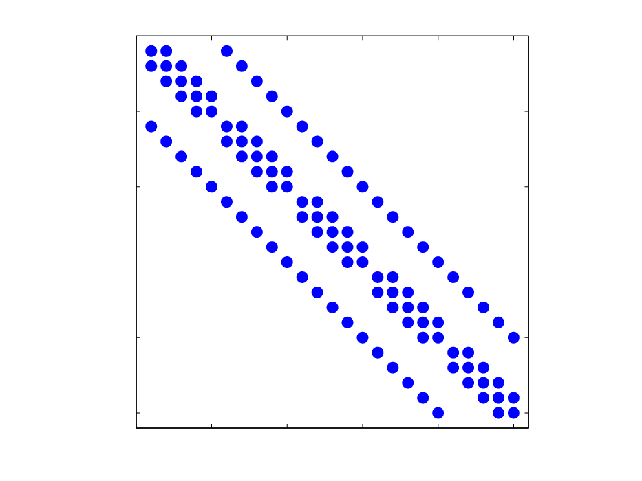
Next, we applied Algorithm 1 to design an optimal sparse controller with the parameters values and , while keeping the performance weights unchanged. It can be observed that the optimal controller cost function increases to , which is about higher, comparing to that of the LQR design. On the other hand, the number of non-zero entries of the controller gain drops to , i.e. . This means a major decrease in the number of non-zero entries of the controller gain. Figures 1a and 1b show the sparsity structure of the system network and the obtained sparse controller. The figures basically visualize the controller matrix by using solid blue circles to represent the non-zero entries of the matrix and leaving the zero entries as blanks. In Figure 1c the graph representation of the generated sparse controller is depicted.
Additionally, we present a brief case study that compares our approach with the Sparsity Promoting Optimal Feedback Control (SPOFC) method, proposed in [54, 26]. The SPOFC method essentially solves a different control problem, since it solves the problem, modified by adding a sparsity promoting penalty function to its cost function and obtain a sub-optimal sparse state feedback controller, while our proposed approach is built upon adjusting the LQR problem to achieve a sparse output feedback controller. Moreover, the approach in SPOFC algorithm fails to directly incorporate the norms bounds on the inputs/outputs and the controller predefined structure. Nonetheless, for comparison purposes and demonstrating the comparable performance of our method, we have obtained the MATLAB source code for SPOFC from the website www.ece.umn.edu/mihailo/sofware/lqrsp, and applied both our method and SPOFC to design sparse state feedback controllers for the randomly generated system. Fig. 2 depicts the results of the simulations performed using both controller design methods. As predicted, the quadratic cost of the closed loop system increases, as the the parameter becomes larger. Moreover, increasing the value of this parameters on the system promotes the sparsity level of feedback gain matrix. Figure 2 depicts the effect of the parameter on the performance of the closed loop system and the number of non-zero entries of the controller gain. In Fig. 2a the -axis represents percentage of the performance loss, which is defined as . The density level percentage of the controller gain is also shown in Fig. 2b when the parameter varies from to .
The simulation results, demonstrated in figure 2, show that the SPOFC approach compromises the performance for a sparser controller in comparison to the our method. Our proposed method assures less performance loss by obtaining denser feedback controller. The disagreement between the optimal solutions of the two algorithms is mainly due to convergence to different local optima. It should also be noted the optimization parameter plays an important, but different, role in adjusting the convergence properties in both of the methods. Hence, setting the parameter to the same value in both optimizations may not be the most accurate choice for the comparison purposes. Moreover, the choice of the system also affects the design performance of both methods. Overall, our extensive simulation results suggest the comparable performance of both approaches. Considering the fact that our problem formulation and solving procedure, which is completely different from the preceding method, generates roughly the same sparse controller, it can be concluded that the derived sparse controller is likely to be the best we can obtain.
VI-B Sub-exponentially Spatially Decaying System


To study the effects of parameters and on the performance of our proposed method, we have run extensive simulations on a randomly generated sub-exponentially spatially decaying system [32]. In such systems, it is assumed the entries of the system matrices decay as they get further from the diagonal, thus we define the matrices and as
where and are uniformly distributed random variables on the open interval . By employing Algorithm 1 till the rank constraint is satisfied, we have depicted the performance degradation and density level of the generated controllers in figure 3 for different values of and . Although the proposed algorithm has converged for all choices of parameters in this simulation, It seems that the choice of the optimization parameter is needed to be at least one order of magnitude larger than the parameter in order to guarantee the convergence to a proper sub-optimal minimum. In addition, since the main objective in designing a sparse controller is to obtain a controller with minimum number of nonzero entries and lowest performance decline, we have also presented the plot of the lowest performance loss obtained for particular values of density level in figure 3c. As expected, it can be observed the performance loss grows as the sprasity level of the controller increases.
VI-C Optimal Sparse Controller with Upper Bound Imposed on the Control Input Norm


In this example, we illustrate the effect of bounding the norm of the control input on the sparsity of the controller matrix. Considering a randomly generated sub-exponential spatially decaying system, with the same parameter values used in section VI-B, we first designed a sparse controller with no constraint on the control input. Our results show that the controllers number of nonzero entries and its performance loss, with respect to the cost of the LQR controller which is , are and respectively. It is also observed that for the generated controller, we have .
We then redesigned the controller, using the re-weighted minimization method, by containing its control input norm in the interval , and obtained controller has the following characteristics: and . Although we bounded the control input norm to an approximately lower value, the obtained controller demonstrates less sparse pattern and higher performance loss. The simulations results, depicted in figure 4, not only verifies the capability of our method to incorporate bounds on the control input, as well as the system output, but also reveals the adverse impact of sparsifying the controller matrix on the control input norm.
VII CONCLUSIONS
In this paper, We have proposed a new framework for optimal sparse output feedback control design, which is capable of incorporating structural constraints on the feedback gain matrix as well as norm bounds on the inputs/outputs of the system. We have shown that problem can be converted to a rank constrained optimization problem with no other non-convex constraints. Using the proposed formulation, we have presented an optimization problem which yields an upper bound for the optimal value of the optimal sparse state feedback control problem. Exploiting the relaxation the -norm with the -norm, We have also expressed that local optimum of the relaxed optimization problem, in its general form, can be obtained by performing ADMM algorithm, which is, in essence, iteratively solving the relaxed problem and projecting its solution to the space of matrices with rank . For the special case, where the objective is merely sparsity pattern recognition of the controller gain, we have demonstrated that the problem can be reduced to an Affine Rank Minimization. The simulation results are also provided to illustrate the utility and performance of our proposed approach. As compared to the results of [26], our results show that while our proposed method has the advantage of performing the output feedback control design restricted by various forms of nonlinear constraints, the performance of our approach is on a par with theirs when applied to the regular sparse state feedback controller design problem.
References
- [1] V. Blondel and J. N. Tsitsiklis, “NP-hardness of some linear control design problems,” SIAM Journal on Control and Optimization, vol. 35, pp. 2118 – 2127, 1997.
- [2] S. Schuler, P. Li, J. Lam, and F. Allgöwer, “Design of structured dynamic output-feedback controllers for interconnected systems,” International Journal of Control, vol. 84, no. 12, pp. 2081–2091, 2011.
- [3] B. Polyak, M. Khlebnikov, and P. Shcherbakov, “An LMI approach to structured sparse feedback design in linear control systems,” in Proceeding of the 2013 European Control Conference, July 2013, pp. 833–838.
- [4] N. Motee and A. Jadbabaie, “Distributed multi-parametric quadratic programming,” IEEE Transactions on Automatic Control, vol. 54, no. 10, pp. 2279–2289, Oct 2009.
- [5] F. Lin, M. Fardad, and M. Jovanovíc, “Augmented Lagrangian approach to design of structured optimal state feedback gains,” IEEE Transactions on Automatic Control, vol. 56, no. 12, pp. 2923–2929, Dec 2011.
- [6] K. Dvijotham, E. Todorov, and M. Fazel, “Convex structured controller design,” CoRR, vol. abs/1309.7731, 2013. [Online]. Available: http://arxiv.org/abs/1309.7731
- [7] B. Bamieh, F. Paganini, and M. A. Dahleh, “Distributed control of spatially-invariant systems,” IEEE Transactions on Automatic Control, vol. 47, pp. 1091–1107, 2002.
- [8] B. Bamieh and P. Voulgaris, “A convex characterization of distributed control problems in spatially invariant systems with communication constraints,” Systems and Control Letters, vol. 54, pp. 575–583, 2005.
- [9] N. Motee and A. Jadbabaie, “Optimal control of spatially distributed systems,” IEEE Transactions on Automatic Control, vol. 53, no. 7, pp. 1616–1629, Aug 2008.
- [10] J. Lavaei, “Optimal decentralized control problem as a rank-constrained optimization,” in 2013 51st Annual Allerton Conference on Communication, Control, and Computing (Allerton), Oct 2013, pp. 39–45.
- [11] G. Fazelnia, R. Madani, A. Kalbat, and J. Lavaei, “Convex relaxation for optimal distributed control problem – Part I: Time-domain formulation,” optimization, vol. 16, p. 17.
- [12] R. Madani, G. Fazelnia, S. Sojoudi, and J. Lavaei, “Low-rank solutions of matrix inequalities with applications to polynomial optimization and matrix completion problems,” Proceedings of the 2014 IEEE Conference on Decision and Control, 2014.
- [13] Y. S. Wang, N. Matni, and J. C. Doyle, “Localized LQR optimal control,” CoRR, vol. abs/1409.6404, 2014.
- [14] Y.-S. Wang and N. Matni, “Localized lqg optimal control for large-scale systems,” submitted to 2015 54th IEEE Conference on Decision and Control (CDC), 2015.
- [15] M. Rotkowitz and S. Lall, “A characterization of convex problems in decentralized control,” IEEE Transactions on Automatic Control, vol. 51, no. 2, pp. 274–286, Feb 2006.
- [16] M. Rotkowitz, “Parametrization of stabilizing controllers subject to subspace constraints,” in American Control Conference (ACC), 2011, June 2011, pp. 5370–5375.
- [17] X. Qi, M. Salapaka, P. Voulgaris, and M. Khammash, “Structured optimal and robust control with multiple criteria: A convex solution,” IEEE Transactions on Automatic Control, vol. 49, no. 10, pp. 1623–1640, Oct 2004.
- [18] D. Donoho, “Compressed sensing,” IEEE Transactions on Information Theory, vol. 52, no. 4, pp. 1289–1306, April 2006.
- [19] R. A. DeVore, “Deterministic constructions of compressed sensing matrices,” Journal of Complexity, vol. 23, no. 4–6, pp. 918 – 925, 2007.
- [20] R. Zahedi, L. Krakow, E. Chong, and A. Pezeshki, “Adaptive estimation of time-varying sparse signals,” IEEE Access, vol. 1, pp. 449–464, 2013.
- [21] R. Zahedi, A. Pezeshki, and E. K. Chong, “Measurement design for detecting sparse signals,” Physical Communication, vol. 5, no. 2, pp. 64 – 75, 2012, compressive Sensing in Communications.
- [22] M. Davenport, P. Boufounos, M. Wakin, and R. Baraniuk, “Signal processing with compressive measurements,” IEEE Journal of Selected Topics in Signal Processing, vol. 4, no. 2, pp. 445–460, April 2010.
- [23] E. Candes and T. Tao, “Decoding by linear programming,” Information Theory, IEEE Transactions on, vol. 51, no. 12, pp. 4203–4215, Dec 2005.
- [24] E. J. Candès, J. K. Romberg, and T. Tao, “Stable signal recovery from incomplete and inaccurate measurements,” Communications on Pure and Applied Mathematics, vol. 59, no. 8, pp. 1207–1223, 2006.
- [25] E. Candes, M. Wakin, and S. Boyd, “Enhancing sparsity by reweighted minimization,” Journal of Fourier Analysis and Applications, vol. 14, pp. 877–905, July 2008.
- [26] F. Lin, M. Fardad, and M. R. Jovanović, “Design of optimal sparse feedback gains via the Alternating Direction Method of Multipliers,” IEEE Transactions on Automatic Control, vol. 58, no. 9, pp. 2426–2431, 2013.
- [27] S. Schuler, C. Ebembauer, and F. Allgöwer, “-system gain and -optimal control,” in Preprints of the 18th IFAC World Congress, August 2011, pp. 9230–9235.
- [28] V. V. Kulkarni, R. Arastoo, A. Bhat, K. Subramanian, M. V. Kothare, and M. C. Riedel, “Gene regulatory network modeling using literature curated and high throughput data,” Systems and Synthetic Biology, vol. 6, no. 3-4, pp. 69–77, December 2012.
- [29] R. Chartrand, “Exact reconstruction of sparse signals via nonconvex minimization,” Signal Processing Letters, IEEE, vol. 14, no. 10, pp. 707–710, Oct 2007.
- [30] M. Lai and J. Wang, “An unconstrained minimization with for sparse solution of underdetermined linear systems,” SIAM Journal on Optimization, vol. 21, no. 1, pp. 82–101, 2011.
- [31] N. Motee and Q. Sun, “Measuring sparsity in spatially interconnected systems,” in 2013 IEEE 52nd Annual Conference on Decision and Control, Dec 2013, pp. 1520–1525.
- [32] ——, “Sparsity and spatial localization measures for spatially distributed systems,” arXiv preprint arXiv:1402.4148, 2014.
- [33] ——, “Sparsity measures for spatially decaying systems,” in Proceedings of the 2014 American Control Conference, June 2014, pp. 5459–5464.
- [34] B. Recht, W. Xu, and B. Hassibi, “Necesary and sufficient conditions for success of the nuclear norm heuristic for rank minimization,” in Proceedings of the 47th IEEE Conference on Decision and Control. Cancun, Mexico, December 2008, pp. 180–185.
- [35] ——, “Null space conditions and thresholds for rank minimization,” Mathematical Programming, vol. 127, pp. 175–211, July 2011.
- [36] M. Mesbahi and G. P. Papavassilopolous, “On the rank minimization problem over a positive semidefinite Linear Matrix Inequality,” IEEE Transacation on Automatic Control, vol. 42, pp. 1239–243, February 1997],.
- [37] B. Recht, M. Fazel, and P. A. Parillo, “Guaranteed minimum rank solutions to Linear Matrix Equations via nuclear norm minimization,” SIAM Review, vol. 52, pp. 471–501, July 2007.
- [38] E. Feron, V. Balakrishnan, S. Boyd, and L. El Ghaoui, “Numerical methods for related problems,” in Proceedings of the 1992 American Control Conference, June 1992, pp. 2921–2922.
- [39] J. Dattoro, Convex Optimization & Euclidean Distance Geometry. Meboo Publishing, 2005.
- [40] R. A. Delgado, J. C. Agüero, and G. C. Goodwin, “A rank-constrained optimization approach: Application to factor analysis,” 19th IFAC World Congress, 2014.
- [41] “Biconvex sets and optimization with biconvex functions: a survey and extensions,” Mathematical Methods of Operations Research, vol. 66, no. 3, 2007.
- [42] S. Boyd, L. El Ghaoui, E. Feron, and V. Balakrishnan, Linear matrix inequalities in system and control theory. SIAM, 1994, vol. 15.
- [43] E. J. Candes, “Compressive sampling,” in International Congress of Mathematicians, vol. III. Zurich: Eur. Math. Soc., December 2006, pp. 1433–1452.
- [44] H. Yu and V. K. N. Lau, “Rank-constrained Schur-convex optimization with multiple trace/log-det constraints,” IEEE Transacation on Signal Processing, vol. 59, pp. 304–314, 2011.
- [45] M. X. Goemans and D. Williamson, “Improved approximation algorithms for maximum cut and satisfiability problems using semidefinite programming,” J. ACM, vol. 42, no. 6, pp. 1115–1145, Nov. 1995.
- [46] “A newton-like method for solving rank constrained linear matrix inequalities,” Automatica, vol. 42, no. 11, pp. 1875 – 1882, 2006.
- [47] M. A. Glowinski, R., “Sur l’approximation, par éléments finis d’ordre un, et la résolution, par pénalisation-dualité d’une classe de problèmes de dirichlet non linéaires,” ESAIM: Mathematical Modelling and Numerical Analysis - Modélisation Mathématique et Analyse Numérique, vol. 9, no. R2, pp. 41–76, 1975.
- [48] D. Gabay and B. Mercier, “A dual algorithm for the solution of nonlinear variational problems via finite element approximation,” Computers & Mathematics with Applications, vol. 2, no. 1, pp. 17 – 40, 1976.
- [49] S. Boyd, N. Parikh, E. Chu, B. Peleato, and J. Eckstein, “Distributed optimization and statistical learning via the Alternating Direction Method of Multipliers,” Foundations and Trends in Machine Learning, vol. 3, pp. 1–124, 2011.
- [50] S. Oymak, A. Jalali, M. Fazel, Y. C. Eldar, and B. Hassibi, “Simultaneously structured models with application to sparse and low-rank matrices,” CoRR, vol. abs/1212.3753, 2012.
- [51] Y. Chen, Y. Chi, and A. Goldsmith, “Estimation of simultaneously structured covariance matrices from quadratic measurements,” in Acoustics, Speech and Signal Processing (ICASSP), 2014 IEEE International Conference on, May 2014, pp. 7669–7673.
- [52] K. Mohan and M. Fazel, “Iterative learning algorithms for matrix rank minimization,” Journal of Machine Learning Research, vol. 13.
- [53] R. Meka, P. Jain, and I. S. Dhillon, “Guaranteed rank minimization via singular value projection,” CoRR, vol. abs/0909.5457, 2009.
- [54] F. Lin, M. Fardad, and M. R. Jovanović, “Sparse feedback synthesis via the Alternating Direction Method of Multipliers,” in Proceedings of the 2012 American Control Conference, 2012, pp. 4765–4770.