The collider experiments have discovered all particles in the standard model (SM), and properties of the SM particles are gradually revealed. Especially, masses of the Higgs boson and top quark are important to investigate a behavior of the quartic coupling of the Higgs boson at a high energy scale. The measurement of Higgs mass showed $125.6\pm 0.35\,{\rm GeV}$ [1], and a recent combine analysis of the collider experiments reported the top mass as $173.34\pm 0.76\,{\rm GeV}$ [2]. A running of the quartic coupling of the Higgs becomes to the negative around $10^{10}\,{\rm GeV}$ GeV by use of the experimental values of the Higgs and top masses. This behavior seems to indicate that our vacuum is metastable.

There are several ways to make the vacuum stable. A simple way is to add an extra scalar to the SM. When we assign odd parity to it under an extra $Z_{2}$ symmetry, it can be a dark matter [3]-[16]. Another way to stabilize the vacuum is modifying runnings of the gauge coupling constants. It decreases (increases) the values of the top Yukawa (Higgs self-) coupling at a high energy, where the vacuum becomes stabilize. In this paper, we try to realize the gauge coupling unification (GCU) at the Planck scale by introducing additional particles in the TeV scale. This extension really induces the above modification of runnings of the gauge coupling constants.

The so-called hierarchy problem is related to the Higgs sector in the SM. A quadratic divergence of the Higgs mass seems to be a dangerous problem. However, the Bardeenfs argument [17] says that it is an unphysical because it can be removed by a subtractive renormalization.¹¹ 1 Reference [18] pointed out the Bardeen’s argument is incorrect, and then discussions of the GCU is changed from ours [19]. However, their conclusions completely depend on the way to deal with gravity. Thus, we do not care about their considerations in this paper. Once it is subtracted and the Higgs mass term is vanishing at the UV scale, it continues to be zero toward the lower energy scale, since the renormalization group equation (RGE) of the Higgs mass term is proportional to itself. We assume a classical conformal symmetry to justify the vanishing Higgs mass term at the high energy scale. This symmetry can be radiatively broken by Coleman-Weinberg mechanism [20]. We can see this situation, for example, in a model with an additional $U(1)$ gauge symmetry and three right-handed neutrinos [21]. Note that the right-handed neutrinos do not change the running of the SM gauge couplings up to the one-loop level, so they are not useful to realize the GCU at the Planck scale.

On the other hand, a logarithmic divergence remains a physical quantity after the renormalization. When there is a heavy particle with the mass, $M$, which couples the Higgs doublet, a quantum correction of $M^{2}\log(\Lambda/\mu)$ causes the hierarchy problem. Thus, naively, we should not introduce any intermediate scales between TeV and UV scales. We assume here that the UV scale is the Planck scale, where all quantum corrections to the Higgs mass are completely vanishing. This assumption requires that corrections from breaking effects of the grand unification at the Planck scale are canceled by a boundary condition of the UV complete theory. Although this assumption seems to be artificial, some UV complete theories, e.g., the string theory, really provides such a boundary condition.

In addition to the above discussion about the hierarchy problem (for example, Ref. [22]), we mention gravity, which involves a specific scale, i.e., the Planck scale. In the point of view of the classical conformal symmetry, there should be no specific scales and no higher-dimensional operators at the classical level. Thus, a certain scale including the Planck scale should be generated by some dynamics. For this purpose, it is known that the Planck scale arises from the vacuum expectation value of a SM gauge singlet scalar, which has a non-minimal coupling with the curvature [23, 24]. Since a mechanism of generating the VEV depends on the hidden sector, the situation is the same as the above discussion in the decoupling limit between the singlet scalar and the Higgs. Then, the hierarchy problem can be solved by a boundary condition at the Planck scale, in which the Higgs mass term is completely vanishing.

For contributions of gravity to the gauge couplings, they could not be ignored around the Planck scale. Then they might upset discussion of the GCU at the Planck scale. To solve this problem, it is known that the GCU could be realized due to the asymptotic safety of gravity, in which all gauge couplings rapidly become zero and approach the same value around the Planck scale. In this scenario, the gravitational contributions have been calculated at lowest nontrivial order in perturbation theory [25]. However, it is pointed out that this calculation depends on a regularization scheme and/or a choice of gauge fixing [26]. In addition, if one applies the dimensional regularization for the calculation, there are no gravitational corrections for the gauge couplings. Thus, we do not consider the gravitational corrections in this paper.

In this paper, we will consider that the Planck scale is the bound of the UV complete theory, in which we assume corrections of the Higgs mass term are completely vanishing at the scale. We also assume that the Higgs mass term is generated by Coleman-Weinberg mechanism and it does not cause the hierarchy problem. In this background, we will consider the GCU at the Planck scale to avoid the introduction of any intermediate scales except for the TeV scale. We introduce extra particles with masses around the TeV scale. In order to avoid the gauge anomaly, the additional fermionic particles are introduced as vector-like. A naive analysis will show that, when all extra particles are fermions and their masses are the same, the GCU at the Planck scale cannot be realized. On the other hand, when extra particles include some scalars, the GCU at the Planck scale can be realized. Then, we find that there are a number of models which can realize the GCU at the Planck scale. Next, we will consider another situation, in which extra fermions have different masses. In this case, models with only extra fermions (no scalars) can realize the GCU around $\sqrt{8\pi}M_{\rm Pl}$. These extensions make the gauge couplings strong enough to realize the GCU, and the top Yukawa (Higgs self-) coupling becomes smaller (larger) than that of the SM at a high energy scale. Then, the vacuum becomes stable.

This paper is composed as follows. At first, we will give a brief review of the vacuum stability and related researches in the SM in Sec. 2. Next, we will investigate possibilities for the realization of GCU at some high energy scales in Sec. 3, and show conditions of the GCU at the Planck scale in Sec. 4. Then, examples of extra particles, which satisfy the conditions, are given in Sec. 5. In addition, we will consider other possibilities, in which the GCU can be realized only by extra fermions, in Sec. 6. Finally, summary and discussion are given in Sec. 7.

We give a brief review of the vacuum stability and related researches in the SM. Realization of the vacuum stability depends on a value of the Higgs quartic coupling $\lambda$. A running of $\lambda$ is obtained by solving the RGE $d\lambda/d\ln\mu=\beta_{\lambda}$, in which $\mu$ is a renormalization scale and $\beta_{\lambda}$ is the $\beta$-function of $\lambda$. The $\beta$-function of $\lambda$ up to two-loop level is given by [27, 28]

	$\displaystyle\beta_{\lambda}$	$\displaystyle=$	$\displaystyle\frac{1}{(4\pi)^{2}}\left[\lambda\left(24\lambda+12y_{t}^{2}-\frac{9}{5}g_{1}^{2}-9g_{2}^{2}\right)-6y_{t}^{4}+\frac{27}{200}g_{1}^{4}+\frac{9}{8}g_{2}^{4}+\frac{9}{20}g_{1}^{2}g_{2}^{2}\right]$		(1)
			$\displaystyle+\frac{1}{(4\pi)^{4}}\left[\lambda^{2}\left(-312\lambda-144y_{t}^{2}+\frac{108}{5}g_{1}^{2}+108g_{2}^{2}\right)+\lambda y_{t}^{2}\left(-3y_{t}^{2}+\frac{17}{2}g_{1}^{2}\right.\right.$
			$\displaystyle\left.+\frac{45}{2}g_{2}^{2}+80g_{3}^{2}\right)+\lambda\left(\frac{1887}{200}g_{1}^{4}-\frac{73}{8}g_{2}^{4}+\frac{117}{20}g_{1}^{2}g_{2}^{2}\right)+y_{t}^{4}\left(30y_{t}^{2}-\frac{8}{5}g_{1}^{2}-32g_{3}^{2}\right)$
			$\displaystyle\left.+y_{t}^{2}\left(-\frac{171}{100}g_{1}^{4}-\frac{9}{4}g_{2}^{4}+\frac{63}{10}g_{1}^{2}g_{2}^{2}\right)-\frac{3411}{2000}g_{1}^{6}+\frac{305}{16}g_{2}^{6}-\frac{1677}{400}g_{1}^{4}g_{2}^{2}-\frac{289}{80}g_{1}^{2}g_{2}^{4}\right],$

where the top Yukawa and the gauge couplings are included. Other Yukawa couplings are omitted, since they are small enough to be neglected. For the Higgs pole mass of $M_{h}=125.7$ GeV and the top pole mass of $M_{t}=173.3$ GeV, $\lambda$ becomes negative at $\mu\simeq 10^{10}$ GeV and the value of $\lambda$ remains negative up to the Planck scale in the SM. As a result, the electroweak (EW) vacuum becomes meta-stable. Thus, one should extend the SM at $\mu\lesssim 10^{10}$ GeV in order to make the vacuum stable with the current center values of Higgs and top masses.

In Fig. 1, we show a relation between the energy, where $\beta_{\lambda}(\mu)=0$ is satisfied, and its value of $\lambda$. For ($M_{h}$, $M_{t}$)=(125.7 GeV, 173.3 GeV), $\lambda$ is minimized at $\mu\simeq 4.0\times 10^{17}$ GeV, and the value is about $-0.0136$. If the minimal value of $\lambda$ is zero with $\beta_{\lambda}=0$ at some high energy scales, the vacua at the EW and the high energy scale are degenerate. This requirement is known as the multiple point criticality principle (MPCP) [29]. Note that the MPCP can be realized at ${\cal O}(10^{17})$ GeV by use of a lighter top mass as 171 GeV (see also Refs. [28] and [30]-[40] for more recent analyses).

From Fig. 1, we can show a minimum of the Higgs potential. It is given by $V_{\rm eff}(\phi)=\frac{1}{4}\lambda\phi^{4}$, where $\phi$ is a field value of the Higgs, and its stationary condition satisfies $\beta_{\lambda}+4\lambda=0$. This equation is satisfied when $|\lambda|$ becomes almost zero, and its solutions are classified in three cases as follows.

• •

  $\lambda=0$ and $\beta_{\lambda}=0$: this is just the MPCP condition, where the height of the potential becomes zero.

• •

  $\lambda>0$ and $\beta_{\lambda}<0$: this point is a local maximum before $\lambda$ becomes a minimal value. If there is another solution for $\lambda>0$ and $\beta_{\lambda}<0$, the point is a local minimum.

• •

  $\lambda<0$ and $\beta_{\lambda}>0$: this point is a global minimum.

For ($M_{h}$, $M_{t}$)=(125.7 GeV, 173.3 GeV), the Higgs potential has a local maximum and global minimum at $\phi\simeq 9.5\times 10^{9}$ GeV and $\phi\simeq 3.9\times 10^{29}$ GeV, respectively.²² 2 In this paper, the strong coupling is taken by $\alpha_{3}(M_{Z})=0.1184$. When $M_{h}$ is larger than 125.7 GeV and/or $M_{t}$ is smaller than 173.3 GeV, the points of local maximum and global minimum are larger and smaller, respectively. For $M_{t}\lesssim 171.2043$ GeV, the potential is positive in any energy scale, and there are no global minimum in the high energy scale. Only for 171.2041 GeV $\lesssim M_{t}\lesssim 171.2043$ GeV, the potential has a local minimum at $4.7\times 10^{17}$ GeV $\lesssim\phi\lesssim 6.1\times 10^{17}$ GeV. When the potential has a plateau around the local minimum, the Higgs inflation can be realized. However, if the Higgs potential includes new contributions as higher order terms of $\phi$, they can significantly affects the vacuum stability [41]-[43].

In this section, we investigate possibilities for the realization of GCU at some high energy scales. In order to see the behavior of the gauge couplings in an arbitrary high energy scale we have to solve the corresponding RGEs. The one-loop level RGEs of the gauge couplings $\alpha_{i}=g_{i}^{2}/4\pi$ are given by

$\displaystyle\frac{d\alpha_{i}^{-1}}{d\ln\mu}=-\frac{b_{i}}{2\pi},$

(2)

where $i=Y$, 2, and 3, and the coefficients of $U(1)_{Y}$, $SU(2)_{L}$, and $SU(3)_{C}$ gauge couplings are given by ($b_{Y}^{\rm SM}$, $b_{2}^{\rm SM}$, $b_{3}^{\rm SM}$)=(41/6, $-19/6$, $-7$) in the SM. $b_{1}^{\rm SM}$ is obtained by multiplying a GUT normalization factor 3/5 to $b_{Y}^{\rm SM}$ as $b_{1}^{\rm SM}=41/10$.³³ 3 Although the normalization factor of hypercharge depends on GUT models, for simplicity, we only consider the factor is 3/5 as in $SU(5)$ GUT. Once particle contents in the model are fixed, values of $b_{i}$ are calculated by [44]

$\displaystyle b_{i}=\left[-\frac{11}{3}c^{i}_{1}+\frac{2}{3}\kappa\sum_{R_{f}}c_{2}(R_{f})\prod_{j\neq i}d_{j}(R_{f})+\frac{1}{3}\eta\sum_{R_{s}}c_{2}(R_{s})\prod_{j\neq i}d_{j}(R_{s})\right],$

(3)

where $j=Y$, 2, and 3. The meanings of the notation are as follows:

• •

  $R_{f}$, $R_{s}$: irreducible chiral fermion and scalar representations, respectively

• •

  $d_{i}(R)$: dimension of the representation $R$ under the gauge groups

• •

  $c_{2}(R)$: quadratic Casimir operator of the representation $R$

• •

  $c^{i}_{1}$: constant usually taken as $c^{i}_{1}=c_{2}(R^{adj})$ ($c^{i}_{1}=N$ for $SU(N)$, and 0 for $U(1)$)

Some values of $c_{2}(R)$ are given in Table 1 in a convention [45, 46]. The factor $\kappa$ is 1 or 1/2 for Dirac or Weyl fermions, respectively. In addition, the factor $\eta$ is 1 or 1/2 for complex or real scalars, respectively. Using the values, we can obtain contributions to $b_{i}$ from fermions and scalars.

Since the GCU is not realized in the SM, one has to extend the SM for the realization of GCU. We will consider adding extra particles with the TeV scale mass to the SM without any additional gauge symmetry. The extra particles with the TeV scale mass are motivated by avoiding the gauge hierarchy problem. Once we fix extra particles, we can easily calculate the values of $b_{i}$ by using Table 1. However, we have to take care of gauge anomalies induced from extra fermions. The simplest way to avoid the anomalies is to add extra fermions as a vector-like form. Thus, in this paper, we will introduce the extra Weyl fermions as a vector-like form except for real representations such as (1,1,0), (1,3,0), (8,1,0), and (8,3,0), which do not yield any gauge anomaly. Although the anomalies can be accidentally canceled as in the SM, we do not consider such cases. Contributions of anomaly free fermions to $b_{i}$ are given in Table 2, which shows only small representations up to an adjoint representation, (8, 3, a). In the same way, contributions from complex scalar particles to $b_{i}$ are given in Table 3. For real scalar particles, contribution to $b_{i}$ is half of the value in Table 3 because of $\eta$ (see Eq. (3)).

Next, we investigate conditions for the GCU. The solution of Eq. (2) are given by

$\displaystyle\alpha_{i}^{-1}(M_{\rm GUT})=\alpha_{i}^{-1}(M_{*})-\frac{b_{i}}{2\pi}\ln\left(\frac{M_{\rm GUT}}{M_{*}}\right),$

(4)

where $M_{*}$ is the mass scale of extra particles and $M_{\rm GUT}$ is the GUT scale, in which the GCU can be realized. The GCU conditions are given by $\alpha_{i}^{-1}(M_{\rm GUT})=\alpha_{j}^{-1}(M_{\rm GUT})\equiv\alpha_{\rm GUT}^{-1}$ for $i,j=1$, 2, and 3. Then, it can be written by

$\displaystyle b^{\prime}_{i}-b^{\prime}_{j}=\frac{2\pi}{\ln\left(\frac{M_{\rm GUT}}{M_{*}}\right)}\left(\alpha_{i}^{-1}(M_{*})-\alpha_{j}^{-1}(M_{*})\right)-(b_{i}^{\rm SM}-b_{j}^{\rm SM}),$

(5)

where $b_{i}=b_{i}^{\rm SM}+b^{\prime}_{i}$, and $b^{\prime}_{i}$ are contributions of the extra particles. Thus, once $M_{*}$ and $M_{\rm GUT}$ are fixed, one can see the required values of $b^{\prime}_{i}$ for the realization of GCU. In the following sections, we investigate possibilities for the realization of GCU at the Planck scale.

In this section, we investigate required values of $b^{\prime}_{i}$ for the realization of GCU at the Planck scale. Substituting $M_{*}=1$ TeV and $M_{\rm Pl}\leq M_{\rm GUT}\leq\sqrt{8\pi}M_{\rm Pl}$ ($M_{\rm Pl}=2.4\times 10^{18}\,{\rm GeV}$) into Eq. (5), we can find that the GCU can be realized when contributions of the extra particles satisfy

	$\displaystyle 2.8\lesssim$	$\displaystyle b^{\prime}_{3}-b^{\prime}_{1}$	$\displaystyle\lesssim 3.2,$		(6)
	$\displaystyle 0.36\lesssim$	$\displaystyle b^{\prime}_{3}-b^{\prime}_{2}$	$\displaystyle\lesssim 0.50,$		(7)

where the lower and upper bounds correspond to $M_{\rm GUT}=M_{\rm Pl}$ and $\sqrt{8\pi}M_{\rm Pl}$, respectively. The RGEs and their boundary conditions in this analysis are given in Appendix.

In addition to these constraint, we impose the conditions of $\alpha_{i}^{-1}(M_{\rm GUT})>0$ to avoid the Landau pole (divergence of gauge couplings). Then, these conditions lead

$\displaystyle b^{\prime}_{i}\lesssim\frac{2\pi}{\ln\left(\frac{M_{\rm GUT}}{M_{*}}\right)}\alpha_{i}^{-1}(M_{*})-b_{i}^{\rm SM}.$

(8)

As a result, $b^{\prime}_{i}$ are limited to

$\displaystyle b^{\prime}_{1}\lesssim 6.1\ (5.7),\qquad b^{\prime}_{2}\lesssim 8.6\ (8.4),\qquad b^{\prime}_{3}\lesssim 9.0\ (8.9),$

(9)

where the values correspond to the $M_{\rm GUT}=M_{\rm Pl}$ ($\sqrt{8\pi}M_{\rm Pl}$) case. Since all $b^{\prime}_{i}$ are positive, gauge couplings become strong compared to those in the SM. In Particular, extra fermions of large representations such as (6, 3, $a$)$\oplus$($\overline{6}$, 3, $-a$) in Table 2 cannot be added to the SM because both $b^{\prime}_{2}$ and $b^{\prime}_{3}$ are larger than the upper bound. Similarly, extra particles with some large representations cannot also be added. Thus, since we need not to consider higher representations than the adjoint representation, extra fermions in Table 2 are sufficient to investigate the realization of GCU.

According to the above discussions, we systematically investigate possibilities of the realization of GCU at the Planck scale, and find that a number of combinations of extra particles satisfy Eq. (10) or (11). For simplicity, we consider representation of extra fermions are the same as the SM fermions (with vector-like partners) and an $SU(2)_{L}$ adjoint fermion as in Table 4. Then, when we consider extra scalars are two $SU(2)_{L}$ doublets (1, 2, 0), the GCU can be realized at $M_{\rm Pl}$ by extra fermions shown in Table 5.⁵⁵ 5 Stable TeV-scale particles with fractional electric charge such as $SU(2)_{L}$ doublet scalar (1, 2, 0) might cause cosmological problems. In order to avoid the problems, the reheating temperature after the inflation should be about 40 times lower than the particle masses [48]. In the case, the corresponding particles cannot be thermally produced in the universe. Thus, since the reheating temperature should be larger than the QCD scale, we consider that it is ${\cal O}(10)\,{\rm GeV}$ in the case. In all cases, masses of extra particles are 1 TeV. The values of the gauge couplings at $M_{\rm GUT}$ are calculated by Eq. (4). They are characterized by $n$ given in Eq. (10), which is shown in the rightmost column. The larger $n$ (equivalently $b_{i}$) becomes, the smaller $\alpha_{\rm GUT}^{-1}$ becomes. We denote the pair of singlets (1, 1, $a$)$\oplus$(1, 1, $-a$) could be used for tuning the running of $g_{1}$ because it only affects $b_{1}$. In addition, we did not list a complete gauge singlet fermion (1, 1, 0), which is usually considered as a right-handed neutrino, because this fermion does not affect the GCU.

For a typical example, we consider the first one of Table 5. In Fig. 3 we show the runnings of gauge and top Yukawa couplings in the extended SM model. Here, we assume that coupling constants of extra particles to the SM particles are negligibly small, and thus introductions of the particles do not significantly change the runnings of top Yukawa and Higgs quartic couplings. The solid and dashed lines correspond to the cases of the extended SM and the SM, respectively. We can see that the GCU is realized at $M_{\rm Pl}$ as mentioned above. In addition, the value of gauge couplings at $M_{\rm GUT}$ is $\alpha_{\rm GUT}^{-1}\simeq 28.0$ as in Table 5.

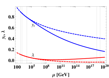
From Fig. 3, we can expect that the Higgs quartic coupling $\lambda$ is positive up to the Planck scale. This reason is understood as follows. In the extended SM, all gauge couplings are large compared to those in the SM because of $b_{i}\geq b_{i}^{\rm SM}$. Then, $y_{t}$ becomes smaller due to the large gauge couplings (see Eq. (19)). Moreover, since $\beta_{\lambda}$ almost depends on quartic terms of $y_{t}$ and $g_{i}$, the smaller $y_{t}$ and the larger $g_{i}$ make $\beta_{\lambda}$ become larger (see Eq. (20)). As a result, $\lambda$ becomes larger, and remains in positive value up to the Planck scale. Even if mixing couplings between the Higgs boson and extra scalars are not negligible, contributions of the mixing couplings to $\beta_{\lambda}$ are positive as long as all of the mixing couplings are positive. On the other hand, when extra fermions couple to the Higgs boson contributions of the couplings to $\beta_{\lambda}$ are negative. Thus, in order to realize the vacuum stability, couplings between the Higgs boson and extra fermions should be small enough to satisfy $\lambda>0$. Note that, when we neglect couplings between the SM particles and extra particles, we can see that $\lambda$ is positive up to the Planck scale.

Next, we consider other situations, in which extra fermions have different masses. In the same way as before, we consider extra fermions within Table 4. Moreover, their masses are taken as $0.5\,{\rm TeV}\leq M\leq 10\,{\rm TeV}$. Actually, we take only lepton masses 0.5 TeV, since lower bounds of vector-like lepton and quark masses are around 200 GeV and 800 GeV, respectively  [49, 50, 51]. Unfortunately, we find that the GCU at $M_{\rm Pl}$ cannot be realized only by extra fermions. In Table 6, we show extra fermions which can realize the GCU around $\sqrt{8\pi}M_{\rm Pl}$. Here, we relax the GCU condition as $\sqrt{8\pi}M_{\rm Pl}\lesssim M_{\rm GUT}\lesssim 2\sqrt{8\pi}M_{\rm Pl}$ because one-loop analyses always have ${\cal O}(1)$ ambiguity. In the table, for example, ”$W\times 1$ (0.5)” shows one (1, 3, 0) fermions with a mass of 0.5 TeV. The reason why the GCU can be realized around $\sqrt{8\pi}M_{\rm Pl}$ is understood by runnings of couplings as a following discussion.

In Fig. 4 we show the runnings of gauge, top Yukawa, and Higgs quartic couplings in the extended SM model which correspond to the first one of Table 6. Here, we assume couplings between the Higgs doublet and extra fermions are negligibly small, and extra fermions do not significantly change running of top Yukawa and Higgs quartic couplings. The solid and dashed lines correspond to the extended SM and the SM, respectively. We can see that the GCU is realized around $\sqrt{8\pi}M_{\rm Pl}$. When extra fermions have different masses, $\beta$-functions of gauge couplings change several times. Then, our previous naive analyses are modified, and values of $M_{\rm GUT}$ shown in Fig. 2 have ${\cal O}(1)$ uncertainty. Thus, the GCU can be realized around $\sqrt{8\pi}M_{\rm Pl}$ by extra fermions with $b^{\prime}_{3}-b^{\prime}_{2}=2/3$. Note that, to realize the vacuum stability, couplings between the Higgs boson and extra fermions should be small as mentioned above.

Finally, we mention the GCU at the string scale ($M_{\rm GUT}=\Lambda_{s}\approx 5.27\times 10^{17}$ GeV). Figure 2 shows that the GCU at the string scale could be realized by $b^{\prime}_{3}-b^{\prime}_{2}=0$, 1/6, and 1/3. The ${\cal O}(1)$ difference could come from two-loop RGEs and one-loop threshold corrections. On the other hand, another possibility is discussed in Ref. [52]. In this paper, the authors consider several possible string-GUT models. Then, the GCU condition is given by

$\displaystyle\alpha_{\rm string}=\frac{2G_{N}}{\alpha^{\prime}}=k_{i}\alpha_{i},$

(12)

where $G_{N}$ and $\alpha^{\prime}$ are the gravitational constant and the Regge slope, respectively. The factor $k_{i}$ ($i=Y$, 2, and 3) is the so-called Ka$\breve{c}$-Moody levels, and the values are different for the considering GUT models [53]. Particularly, $k_{2}$ and $k_{3}$ should be positive integer, and we take Ka$\breve{c}$-Moody levels as ($k_{Y}$, $k_{2}$, $k_{3}$) = (5/3, 1, 1), which are given in GUT models such as $SU(5)$ and $SO(10)$. However, for $k_{2}\neq 1$ and/or $k_{3}\neq 1$, the GCU conditions of our analyses are changed. When the new physic scale is $M_{*}=1$ TeV, the GCU at $\Lambda_{s}$ can be realized by

$\displaystyle\frac{b^{\prime}_{3}}{2}-b^{\prime}_{2}\simeq-4.34\approx-\frac{13}{3},\qquad\frac{b^{\prime}_{3}}{2}-\frac{3}{13}b^{\prime}_{1}\simeq 1.99$

(13)

for ($k_{Y}$, $k_{2}$, $k_{3}$) = (13/3, 1, 2), which is given in the GUT model as $SU(5)\times SU(5)$ and $SO(10)\times SO(10)$. In the same way, the GCU at $\Lambda_{s}$ can be realized by

$\displaystyle b^{\prime}_{3}-\frac{b^{\prime}_{2}}{2}\simeq 4.64\approx\frac{14}{3},\qquad b^{\prime}_{3}-\frac{3}{2}b^{\prime}_{1}\simeq-7.46$

(14)

for ($k_{Y}$, $k_{2}$, $k_{3}$) = (2/3, 2, 1), which is given in the GUT model as $E_{7}$. Both conditions can be satisfied only by extra fermions due to $b^{\prime}_{3}/2-b^{\prime}_{2}\propto 1/3$ and $b^{\prime}_{3}-b^{\prime}_{2}/2\propto 1/3$. Thus, in some string-GUT models, the GCU at $\Lambda_{s}$ can be realized only by extra fermions.

We have explored possibilities of GCU at the Planck scale in the extended SM which includes extra particles around the TeV scale. To avoid the gauge anomaly, extra fermions are constrained as vector-like and adjoint representations. When all extra particles are fermions and their masses are the same, the GCU at the Planck scale cannot be realized (up to one-loop level). On the other hand, when extra particles include some scalar particles there are two cases which realize the GCU at the Planck scale. The conditions of the GCU at $M_{\rm Pl}$ and $\sqrt{8\pi}M_{\rm Pl}$ are given by Eqs. (10) and (11), respectively. Then, we have found that there are a number of combinations which satisfy these equations. For examples, when extra scalars are two $SU(2)_{L}$ doublets as (1, 2, 0), the GCU at $M_{\rm Pl}$ are realized by extra fermions given in the leftmost column of Table 5.

Moreover, we have considered other situations, in which extra fermions have different masses. In this case, extra fermions can realize the GCU around $\sqrt{8\pi}M_{\rm Pl}$ as in Table 6. Since $\beta$-functions of gauge couplings change several times by extra fermions with different masses, our previous naive analyses are modified, and the GCU can be realized around $\sqrt{8\pi}M_{\rm Pl}$. Note that, if we use the two-loop RGEs and one-loop threshold corrections, these results could change, and other possibilities could exist.

If there are no intermediate scales between the TeV scale and the GCU scale, and quantum corrections to the Higgs mass term are completely vanishing at the GCU scale due to a UV-complete theory, the Higgs mass receives quantum corrections only from TeV scale particles. In this paper, we have assumed that the GCU scale is the Planck scale, and the Higgs mass term are vanishing at the scale. More detailed discussion has been done in the introduction and Ref. [22]. When the GCU at the Planck scale is realized, gauge couplings become larger compared to the SM case. Then, top Yukawa and Higgs quartic couplings become smaller and larger, respectively. As a result, the vacuum can be stable up to the Planck scale.

Finally, we mention the proton lifetime in a GUT model. Although we do not discuss any specific GUT model, the proton lifetime should be long enough to avoid the experimental lower bound. The proton lifetime is usually given by

$\displaystyle\tau_{\rm proton}\sim\left(\alpha_{i}^{-1}(M_{\rm GUT})\right)^{2}\frac{M_{\rm GUT}^{4}}{m_{\rm proton}^{5}}.$

(15)

This is derived from a four-fermion approximation for the decay channel $p\rightarrow e^{+}+\pi^{0}$. For $M_{\rm GUT}\simeq M_{\rm Pl}$, we obtain $\tau_{\rm proton}\sim\left(\alpha_{i}^{-1}(M_{\rm GUT})\right)^{2}\times 10^{42}$ yrs. Since $\alpha_{i}^{-1}(M_{\rm GUT})$ is larger than 1 (see Table 5), the proton lifetime is much longer than the experimental lower bound.

References

- [1] T. Hahn, S. Heinemeyer, W. Hollik, H. Rzehak and G. Weiglein, arXiv:1404.0186 [hep-ph].
- [2] [ATLAS and CDF and CMS and D0 Collaborations], arXiv:1403.4427 [hep-ex].
- [3] V. Silveira and A. Zee, Phys. Lett. B 161, 136 (1985).
- [4] J. McDonald, Phys. Rev. D 50, 3637 (1994) [hep-ph/0702143 [HEP-PH]].
- [5] C. P. Burgess, M. Pospelov and T. ter Veldhuis, Nucl. Phys. B 619, 709 (2001) [hep-ph/0011335].
- [6] H. Davoudiasl, R. Kitano, T. Li and H. Murayama, Phys. Lett. B 609, 117 (2005) [hep-ph/0405097].
- [7] B. Grzadkowski and J. Wudka, Phys. Rev. Lett. 103, 091802 (2009) [arXiv:0902.0628 [hep-ph]].
- [8] B. Grzadkowski and J. Wudka, Acta Phys. Polon. B 40, 3007 (2009) [arXiv:0910.4829 [hep-ph]].
- [9] A. Drozd, B. Grzadkowski and J. Wudka, JHEP 1204, 006 (2012) [Erratum-ibid. 1411, 130 (2014)] [arXiv:1112.2582 [hep-ph]].
- [10] M. Kadastik, K. Kannike, A. Racioppi and M. Raidal, JHEP 1205, 061 (2012) [arXiv:1112.3647 [hep-ph]].
- [11] S. Baek, P. Ko and W. I. Park, JHEP 1307, 013 (2013) [arXiv:1303.4280 [hep-ph]].
- [12] N. Haba, K. Kaneta and R. Takahashi, Phys. Lett. B 734, 220 (2014) [arXiv:1309.1231 [hep-ph]].
- [13] N. Haba, K. Kaneta and R. Takahashi, Eur. Phys. J. C 74, 2696 (2014) [arXiv:1309.3254 [hep-ph]].
- [14] N. Haba, K. Kaneta and R. Takahashi, JHEP 1404, 029 (2014) [arXiv:1312.2089 [hep-ph]].
- [15] E. Gabrielli, M. Heikinheimo, K. Kannike, A. Racioppi, M. Raidal and C. Spethmann, Phys. Rev. D 89, 015017 (2014) [arXiv:1309.6632 [hep-ph]].
- [16] S. M. Boucenna, S. Morisi, Q. Shafi and J. W. F. Valle, Phys. Rev. D 90, 055023 (2014) [arXiv:1404.3198 [hep-ph]].
- [17] W. A. Bardeen, FERMILAB-CONF-95-391-T, C95-08-27.3.
- [18] G. Marques Tavares, M. Schmaltz and W. Skiba, Phys. Rev. D 89, no. 1, 015009 (2014) [arXiv:1308.0025 [hep-ph]].
- [19] G. F. Giudice, G. Isidori, A. Salvio and A. Strumia, JHEP 1502, 137 (2015) [arXiv:1412.2769 [hep-ph]].
- [20] S. R. Coleman and E. J. Weinberg, Phys. Rev. D 7, 1888 (1973).
- [21] S. Iso, N. Okada and Y. Orikasa, Phys. Lett. B 676, 81 (2009) [arXiv:0902.4050 [hep-ph]].
- [22] S. Iso and Y. Orikasa, PTEP 2013, 023B08 (2013) [arXiv:1210.2848 [hep-ph]].
- [23] A. Zee, Phys. Rev. Lett. 42, 417 (1979).
- [24] R. Foot, A. Kobakhidze, K. L. McDonald and R. R. Volkas, Phys. Rev. D 77, 035006 (2008) [arXiv:0709.2750 [hep-ph]].
- [25] S. P. Robinson and F. Wilczek, Phys. Rev. Lett. 96, 231601 (2006) [hep-th/0509050].
- [26] A. R. Pietrykowski, Phys. Rev. Lett. 98, 061801 (2007) [hep-th/0606208].
- [27] C. Ford, I. Jack and D. R. T. Jones, Nucl. Phys. B 387, 373 (1992) [Erratum-ibid. B 504, 551 (1997)] [hep-ph/0111190].
- [28] D. Buttazzo, G. Degrassi, P. P. Giardino, G. F. Giudice, F. Sala, A. Salvio and A. Strumia, JHEP 1312, 089 (2013) [arXiv:1307.3536].
- [29] C. D. Froggatt and H. B. Nielsen, Phys. Lett. B 368, 96 (1996) [hep-ph/9511371].
- [30] M. Holthausen, K. S. Lim and M. Lindner, JHEP 1202, 037 (2012) [arXiv:1112.2415 [hep-ph]].
- [31] F. Bezrukov, M. Y. Kalmykov, B. A. Kniehl and M. Shaposhnikov, JHEP 1210, 140 (2012) [arXiv:1205.2893 [hep-ph]].
- [32] G. Degrassi, S. Di Vita, J. Elias-Miro, J. R. Espinosa, G. F. Giudice, G. Isidori and A. Strumia, JHEP 1208, 098 (2012) [arXiv:1205.6497 [hep-ph]].
- [33] S. Alekhin, A. Djouadi and S. Moch, Phys. Lett. B 716, 214 (2012) [arXiv:1207.0980 [hep-ph]].
- [34] I. Masina, Phys. Rev. D 87, no. 5, 053001 (2013) [arXiv:1209.0393 [hep-ph]].
- [35] Y. Hamada, H. Kawai and K. y. Oda, Phys. Rev. D 87, no. 5, 053009 (2013) [Erratum-ibid. D 89, no. 5, 059901 (2014)] [arXiv:1210.2538 [hep-ph]].
- [36] F. Jegerlehner, Acta Phys. Polon. B 45, 1167 (2014) [arXiv:1304.7813 [hep-ph]].
- [37] I. Masina and M. Quiros, Phys. Rev. D 88, 093003 (2013) [arXiv:1308.1242 [hep-ph]].
- [38] A. Spencer-Smith, arXiv:1405.1975 [hep-ph].
- [39] N. Haba, H. Ishida, K. Kaneta and R. Takahashi, Phys. Rev. D 90, 036006 (2014) [arXiv:1406.0158 [hep-ph]].
- [40] N. Haba, K. Kaneta, R. Takahashi and Y. Yamaguchi, arXiv:1408.5548 [hep-ph].
- [41] V. Branchina and E. Messina, Phys. Rev. Lett. 111, 241801 (2013) [arXiv:1307.5193 [hep-ph]].
- [42] V. Branchina, E. Messina and M. Sher, Phys. Rev. D 91, no. 1, 013003 (2015) [arXiv:1408.5302 [hep-ph]].
- [43] V. Branchina, E. Messina and A. Platania, JHEP 1409, 182 (2014) [arXiv:1407.4112 [hep-ph]].
- [44] D. R. T. Jones, Phys. Rev. D 25, 581 (1982).
- [45] R. Slansky, Phys. Rept. 79, 1 (1981).
- [46] M. Lindner and M. Weiser, Phys. Lett. B 383, 405 (1996) [hep-ph/9605353].
- [47] G. F. Giudice and A. Romanino, Nucl. Phys. B 699, 65 (2004) [Erratum-ibid. B 706, 65 (2005)] [hep-ph/0406088].
- [48] D. J. H. Chung, E. W. Kolb and A. Riotto, Phys. Rev. D 60, 063504 (1999) [hep-ph/9809453].
- [49] S. Chatrchyan et al. [CMS Collaboration], Phys. Lett. B 718, 348 (2012) [arXiv:1210.1797 [hep-ex]].
- [50] S. Chatrchyan et al. [CMS Collaboration], Phys. Lett. B 729, 149 (2014) [arXiv:1311.7667 [hep-ex]].
- [51] G. Aad et al. [ATLAS Collaboration], JHEP 11, 104 (2014) [arXiv:1409.5500 [hep-ex]].
- [52] V. Barger, J. Jiang, P. Langacker and T. Li, Int. J. Mod. Phys. A 22, 6203 (2007) [hep-ph/0612206].
- [53] A. Perez-Lorenzana and W. A. Ponce, Europhys. Lett. 49, 296 (2000) [hep-ph/9911540].