Quark star model with charged anisotropic matter
Abstract
We find two new classes of exact solutions to the Einstein-Maxwell system of equations. The matter distribution satisfies a linear equation of state consistent with quark matter. The field equations are integrated by specifying forms for the measure of anisotropy and a gravitational potential which are physically reasonable. The first class has a constant potential and is regular in the stellar interior. It contains the familiar Einstein model as a limiting case and we can generate finite masses for the star. The second class has a variable potential and singularity at the centre. A graphical analysis indicates that the matter variables are well behaved.
Key words: Gravitational potential; linear equation of state; quark matter; measure of anisotropy.
Permanent address: School of Mathematical Sciences, University of Dodoma, Tanzania.00footnotetext: Astrophysics and Cosmology Research Unit, School of Mathematics, Statistics and Computer Science, University of KwaZulu-Natal, Private Bag X54001, Durban 4000, South Africa.00footnotetext: Astrophysics and Cosmology Research Unit, School of Mathematics, Statistics and Computer Science, University of KwaZulu-Natal, Private Bag X54001, Durban 4000, South Africa.
I Introduction
The nonlinear Einstein-Maxwell field equations are necessary for the description of the behaviour of relativistic gravitating matter with or without electromagnetic field distributions, and they are tools for modeling relativistic compact objects such as dark energy stars, gravastars, quark stars, black holes and neutron stars. With the help of diverse solutions of the field equations and different matter configurations, the structure and properties of relativistic stellar bodies have been investigated. This is reflected in several investigations over the recent past. Models of neutral compact spheres with isotropic pressures have been studied by [38], [32], and [42]. The case of neutral anisotropic matter was investigated by [40], [16] and [21, 20]. Charged isotropic compact models are highlighted by [14, 15], [39], [37], and [1]. The general model with charge and anisotropy was analysed by Esculpi and Aloma (2010), [25] and [41]. Several interesting features of exact solutions to the Einstein-Maxwell system for charged anisotropic quark stars were highlighted in the treatments of [29] and Sunzu et al. (2014).
The effect of the electromagnetic distribution and pressure anisotropy are important ingredients to be considered when undertaking studies of relativistic stellar objects. [19] highlighted the fact that the presence of charge in a compact stellar matter contributes to changes in the mass, redshift and luminosity. It was shown by [43] that charged models could allow causal signals in the stellar interior over a wide range of parameters. On the other hand, [4] demonstrated that pressure anisotropy affects the physical properties, stability and structure of stellar matter. The stability of stellar bodies is improved for positive measure of anisotropy when compared to configurations of isotropic stellar objects. Furthermore the maximum mass and the redshift depend on the magnitude of the pressure anisotropy as illustrated by [5] and [12]. They also showed that the presence of anisotropic pressures in charged matter enhances the stability of the configuration under radial adiabatic perturbations when compared to isotropic matter. There have been many recent investigations which include the presence of charge and anisotropy in the stellar interior. For example, [27] presented regular models for charged anisotropic stellar bodies, generalized isothermal models were found by [28], and superdense models were investigated by [36]. Other new exact solutions for charged anisotropic stars are contained in the treatment of Maharaj and Mafa Takisa (2012). Some other models describing anisotropic static spheres with variable energy density include the works of Cosenza et al. (1981), [13] and Herrera and Santos (1997).
On physical grounds for a stellar model we should include a barotropic equation of state so that the radial pressure is a function of the energy density. Exact models of charged anisotropic matter with a quadratic equation of state were found by [10]. Using the same equation of state, Maharaj and Mafa Takisa (2012) generated regular models for charged anisotropic stars. A strange star model with a quadratic equation of state was recently generated by [35]. Polytropic models were analysed by [26] for charged matter with anisotropic stresses. [33, 34] found charged stellar models with a Van der Waals and generalized Van der Waals equation of state respectively. Anisotropic models with a modified Van der Waals equations of state are contained in the paper by [48]. Other relativistic stellar models with a Van der Waals equation of state are studied in the treatment of [24]. However for a quark star we require a linear equation of state. The first treatment of quark stars was undertaken by [18] for hydrostatic matter in equilibrium. Since then there have been many investigations on the study of structure and properties of quark matter by adopting a linear equation of state. It has been shown by [51], [2], Farhi and Jaffe (1984) that quark matter could be studied with the aid of the phenomenology of the MIT bag model; these studies indicate that a linear quark matter equation of state with a nonzero bag constant can be used. The review by [50] described the astrophysical phenomenology of compact quark stars. The study of nonradial oscillations of quark stars was performed by [45] and [44]. Charged isotropic models for quark stars are described by [31] and Komathiraj and Maharaj (2007). Particular models have been analysed to study the effect of both the electric field and the anisotropy in quark stars are those generated by Rahaman et al. (2012), [21], [30], [49], [47], Maharaj and Thir-ukkanesh (2009b) and [8]. However most charged anisotropic models of quark stars have anisotropy always present and do not regain isotropic pressures as a special case. Charged anisotropic models for quark stars that allow anisotropy to vanish have been found in the papers by [29] and [46].
The objective of this paper is to find new exact solutions to the Einstein-Maxwell system of equations with a linear quark matter equation of state for charged anisotropic stars. We build new models by specifying a particular form for one of the gravitational potentials and the measure of anisotropy. The model allows us to regain isotropic pressures as a special case. To achieve this objective we structure this paper accordingly. In Section II we give the fundamental equations and transformation of the field equations according to [7] and incorporate the linear quark matter equation of state. We then specify a new form for one of the gravitational potential and the measure of anisotropy which are physically viable and reasonable. This helps to deduce the master differential equation governing the behaviour of our model. In Section III we generate a regular model and regain the Einstein model with isotropic pressures. We show that this class produces objects with finite mass. In Section IV we find a second class of solutions. This class has variable potentials and singularity at the centre. In Section V we give graphical analysis and make concluding remarks.
II Fundamental equations
We intend to describe stellar structure with quark matter in a general relativistic setting. The spacetime manifold must be static and spherically symmetric. The interior spacetime is given by the metric
| (1) |
where and are arbitrary functions. The Reissner-Nordstrom line element describes the exterior spacetime
| (2) | |||||
where and represent total mass and charge as measured by an observer at infinity. The energy momentum tensor
| (3) | |||||
describes anisotropic charged matter. The energy density , the radial pressure , the tangential pressure , and the electric field intensity are measured relative to a vector u. The vector is comoving, unit and timelike.
The Einstein-Maxwell equations with matter and charge can be written as
| (4a) | |||||
| (4b) | |||||
| (4c) | |||||
| (4d) | |||||
where primes indicate differentiation with respect to the radial coordinate . The quantity denotes the proper charge density. Note that we are using units where the coupling constant and the speed of light . The mass contained within the charged sphere is defined by
| (5) |
where is the energy density when the electric field . For a quark star we have a linear relationship between the radial pressure and the energy density
| (6) |
where is the bag constant.
We transform the field equations to an equivalent form by introducing a new independent variable and defining metric functions and as
| (7) |
where and are arbitrary constants. With this transformation the line element in (1) becomes
| (8) |
The mass function (5) becomes
| (9) |
where
| (10) |
and a dot represents differentiation with respect to the variable .
Then we can write the Einstein-Maxwell field equations (4), with the quark equation of state (6), in the following form
| (11a) | |||||
| (11b) | |||||
| (11c) | |||||
| (11d) | |||||
| (11e) | |||||
| (11f) | |||||
The gravitational behaviour of the anisotropic charged quark star is governed by the system (11). The quantity is called the measure of anisotropy. The system of equations (11) consists of eight variables in six equations. The advantage of the Einstein-Maxwell system (11) is that it has a simple representation: it is given in terms of the matter variables , the charged quantities and the gravitational potentials and . We rewrite (11d) in a more simplified form as
| (12) |
This is a highly nonlinear equation in general. However if and are given functions then the form (12) of the field equation is linear in the variable . In order to find exact solutions to this model we will specify the two quantities and .
We choose the metric function as
| (13) |
where , , and are constants. This choice guarantees that the metric function is continuous and well behaved within the interior of the star for a range of values of and . The metric function is also finite at the centre of the star. We specify the measure of anisotropy in the form
| (14) |
where are arbitrary constants. A similar choice of anisotropy was made by [29]. This choice is physically reasonable as it is continuous and well behaved throughout the interior of the star. It is finite at the centre of the star. It is possible to regain isotropic pressures when . We then have and the anisotropy vanishes. Substituting (13) and (14) in (12) we obtain the first order differential equation
| (15) |
where we have set
for convenience.
| radius (km) | mass () | model | |||||
|---|---|---|---|---|---|---|---|
| 28.0 | 1.0 | 1.1 | 2.2 | 1.8 | 9.46 | 2.86 | [31] |
| 13.0 | 1.0 | 11.0 | 9.0 | 5.0 | 10.99 | 2.02 | [39] |
| 17.0 | 1.0 | 13.5 | 10.0 | 8.0 | 9.40 | 1.67 | [11] |
| 30.54 | 1.0 | 20.51 | 25.0 | 30.0 | 7.60 | 1.60033 | [46] |
| 34.0 | 1.0 | 28.6 | 35.0 | 20.0 | 7.07 | 1.433 | [6] |
| 33.93 | 1.0 | 40.4 | 24.0 | 20.0 | 6.84 | 1.28994 | [46] |
| 22.18 | 1.0 | 10.5 | 4.0 | 5.0 | 7.07 | 0.94 | [47] |
III A regular model
As solution to (15) is desirable. We can find a nonsingular exact model for the choice of values of the parameters
With these values the potential and (15) becomes
| (16) |
Solving the above differential equation we obtain
| (17) |
Using the system (11) we obtain the exact solution describing the potentials and matter variables as
| (18a) | |||||
| (18b) | |||||
| (18c) | |||||
| (18d) | |||||
| (18e) | |||||
| (18f) | |||||
| (18g) | |||||
where
This model admits no singularity in the interior in the potentials and in the matter variables. In addition and at the stellar centre.
With this model the line element (8) becomes
| (19) | |||||
Using the system (18), the mass function (9) becomes
| (20) |
In this exact solution we regain the special case of vanishing anisotropy and charge: and . Then the potentials and matter variables become
| (21) |
with the line element
| (22) | |||||
in terms of the variable .
Note that we can write (22) in the equivalent form
| (23) | |||||
where . We observe that (23) is the familiar uncharged Einstein model with isotropic pressure and the equation of state . We can therefore interpret the exact solution (18) as a generalized Einstein model with charge and anisotropy. This possibility arises only because the energy density at the boundary is a nonzero constant in a quark star.
The solutions found in this section do represent finite masses that can be related to observed objects. To show this we introduce the
transformations
, ,
, , .
Based on these transformations we choose values of parameters to generate stellar masses and radii in Table 1. For computation purposes
we have set .
Therefore we generate masses in the range contained in the investigations of [31],
[39], [11], [46], [6] and
[47]. Therefore the exact solutions of this section do in fact produce finite masses consistent with masses of physically reasonable
astronomical objects.
IV Generalized models
It is possible that other exact solutions exist, in addition to those found above, and which may be obtained using the approach of this paper. Clearly these new solutions will correspond to different matter distributions, and consequently have different energy density profiles to the Einstein-Maxwell model considered in Section III. The choice of parameters we made in Section III led to constant . Here we again choose , but we take . Then the gravitational potential is no longer constant. Consequently (15) can be written in the form
| (24) |
Equation (24) is more complicated that (16) but it can be integrated. Solving (24) we obtain the function
| (25) |
where
Note that when then we have isotropic pressures. The function (25) demonstrates that there are other exact solutions to the differential equation (12) in terms of elementary functions.
Using the field equations indicated in the system (11) we obtain the following exact solution
| (26a) | |||||
| (26b) | |||||
| (26c) | |||||
| (26d) | |||||
| (26e) | |||||
| (26f) | |||||
| (26g) | |||||
where we have set
for convenience.
Based on our exact solution in the system (26), the line element in (8) becomes
| (27) | |||||
The mass function has the form
| (28) | |||||
Therefore we have obtained another exact solution to the Einstein-Maxwell system of equations (11) with a quark equation of state. Other solutions to (15) are possible for different choices of parameters , , and . It is not clear that other choices are likely to easily produce tractable forms for gravitational potential . The advantage of the exact solutions (18) and (26) is that they have a simple form. They are expressed in terms of elementary functions. The model (26) is singular at the centre. This is a feature that is shared with the quark star model of [31] but the stellar mass and electric field remain finite.
V Discussion
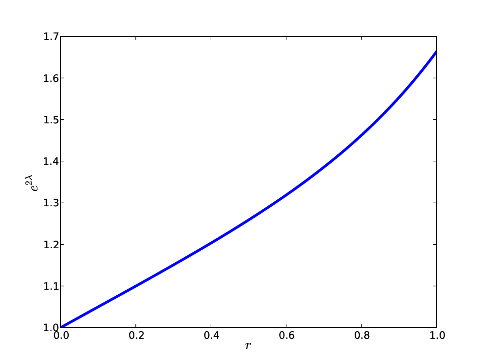
In this section we indicate that the exact solution of the field equations (26) is well behaved away from the centre. To do this we consider the behaviour of the gravitational potentials, matter variables and the electric field. We note that , and , so that the energy density, the radial pressure and the tangential pressure are decreasing functions. The gradients are greatest in the central core regions. This happens because the profiles for , and are dominated by the presence of the term containing the factor . Other choices for the parameters , , and in (15) could lead to models with gradients where the rate of change is more gradual. The Python programming language was used to generate graphical plots for the remaining quantities of physical interest for the particular choices , , , , , , and . The graphical plots generated are for the potential (Fig. 1), potential (Fig. 2), measure of anisotropy (Fig. 3), the electric field (Fig. 4) and the mass (Fig. 5). All figures are plotted against the radial coordinate . Most of these quantities are regular and well behaved in the stellar interior except for the electric field which is divergent at the centre. In this case our exact solutions may describe the outer regions, away from the centre, in a core envelope model. However, note that the gravitational potentials, the measure of anisotropy and the mass remain finite, regular and well behaved throughout the interior of the stellar structure. In general the measure of anisotropy is finite and a continuous decreasing function as shown in Fig. 3. A similar profile of the anisotropy was obtained by [21] and [22]. The mass is an increasing function of the radial distance as indicated in Fig. 5.
We have found exact solutions for the Einstein-Maxwell equations for anisotropic charged quark matter. We have considered the spacetime geometry of the stellar interior to be static and spherically symmetric. The linear equation of state, consistent with quark matter, has been incorporated in our models. The solutions to the field equations are found after making a reasonable physical choice for the measure of anisotropy and one of the gravitational potentials. We have analysed two models: the first is regular throughout the interior in the matter variables and gravitational potentials, and the second is a generalized model that admits a singularity in some of the matter variables at the centre of the stellar object. We have regained masses and radii consistent with the [31], [39], [11], [46], [6] and [47] models. We believe that our toy models may facilitate studies of anisotropic quark stars with an electromagnetic field distribution and provide room for further studies of other relativistic matter distributions. This may be achieved with a specific equation of state, spacetime geometry and metric functions different from what we have considered in this paper.



Acknowledgements
We are grateful to the National Research Foundation and the University of KwaZulu-Natal for financial support. SDM acknowledges that this work is based upon research supported by the South African Research Chair Initiative of the Department of Science and Technology. JMS extends his appreciation to the University of Dodoma in Tanzania for study leave.
References
- [1] Bijalwan, N.: Astrophys. Space Sci. 336, 413 (2011)
- [2] Chodos, A., Jaffe, R.L., Johnson, K., Thom, C.B., Weisskopf, V.F.: Phys. Rev. D 9, 3471 (1974)
- [3] Cosenza, M., Herrera, L., Esculpi, M., Witten, L.: J. Math. Phys. 22, 118 (1981)
- [4] Dev, K., Gleiser, M.: Gen. Relativ. Gravit. 34, 1793 (2002)
- [5] Dev, K., Gleiser, M.: Gen. Relativ. Gravit. 35, 1435 (2003)
- [6] Dey, M., Bombaci I., Dey, J., Ray S., Samanta, B.C.: Phys. Lett. B 438, 123 (1998)
- [7] Durgapal, M.C., Bannerji, R.: Phys. Rev. D 27, 328 (1983)
- [8] Esculpi, M., Aloma, E.: Eur. Phys. J. C 67, 521 (2010)
- [9] Farhi, E., Jaffe, R.L.: Phys. Rev. D 30, 2379 (1984)
- [10] Feroze, T., Siddiqui, A.A.: Gen. Relativ. Gravit. 43, 1025 (2011)
- [11] Freire, P.C.C, Bassa, C.G., Wex, N., Stairs, I.H. et al: Mon. Not. R. Astron. Soc. 412, 2763 (2011)
- [12] Gleiser, M., Dev, K.: Int. J. Mod. Phys. D 13, 1389 (2004)
- [13] Gokhroo, M.K., Mehra, A.L.: Gen. Relativ. Gravit. 26, 75 (1994)
- [14] Gupta, Y.K., Maurya, S.K.: Astrophys. Space Sci. 332, 155 (2011a)
- [15] Gupta, Y.K., Maurya, S.K.: Astrophys. Space Sci. 331, 135 (2011b)
- [16] Harko, T., Mak, M.K.: Annalen Phys. 11, 3 (2002)
- [17] Herrera, L., Santos, N.O.: Phys. Rep. 286, 53 (1997)
- [18] Itoh, N.: Prog. Theor. Phys. 44, 291 (1970)
- [19] Ivanov, B.V.: Phys. Rev. D 65, 104001 (2002)
- [20] Kalam, M., Rahaman, F., Ray, S., Hossein, Sk.M., Karar, I., Naska, J.: Eur. Phys. J. C 72, 2248 (2012)
- [21] Kalam, M., Usmani, A.A., Rahamani F., Hossein, S.M., Karar, I., Sharma, R.: Int. J. Theor. Phys. 52, 3319 (2013)
- [22] Karmakar, S., Mukherjee, S., Sharma, R., Maharaj, S.D.: Pramana - J. Phys. 68, 881 (2007)
- [23] Komathiraj, K., Maharaj, S.D.: Int. Mod. Phys. D 16, 1803 (2007)
- [24] Lobo, F.S.N.: Phys. Rev. D 75, 024023 (2007)
- [25] Mafa Takisa, P., Maharaj, S.D.: Astrophys. Space Sci. 343, 569 (2013a)
- [26] Mafa Takisa, P., Maharaj, S.D.: Gen. Relativ. Gravit. 45, 1951 (2013b)
- [27] Maharaj, S.D., Mafa Takisa, P.: Gen. Relativ. Gravit. 44, 1419 (2012)
- [28] Maharaj, S.D., Thirukkanesh, S.: Pramana - J. Phys. 72, 481 (2009)
- [29] Maharaj, S.D., Sunzu, J.M., Ray, S.: Eur. Phys. J. Plus 129, 3 (2014)
- [30] Mak, M.K., Harko T.: Chin. J. Astron. Astrophys. 2, 248 (2002)
- [31] Mak, M.K., Harko, T.: Int. J. Mod. Phys. D 13, 149 (2004)
- [32] Mak, M.K., Harko, T.: Pramana - J. Phys. 65, 185 (2005)
- [33] Malaver, M.: World Applied Programming 3, 309 (2013a)
- [34] Malaver, M.: American Journal of Astronomy and Astrophysics 1, 41 (2013b)
- [35] Malaver, M..: Frontiers of Mathematics and its Applications 1, 9 (2014)
- [36] Maurya, S.K., Gupta, Y.K.: Phys. Scr. 86, 025009 (2012)
- [37] Murad, M.H., Fatema, S.: Astrophys. Space Sci. 344, 69 (2013)
- [38] Murad, M.H., Pant, N.: Astrophys. Space Sci. 350, 349 (2014)
- [39] Negreiros, R.P., Weber, F., Malheiro, M., Usov, V.: Phys. Rev. D 80, 083006 (2009)
- [40] Paul, B.C., Chattopadhyay, P.K., Karmakar, S., Tikekar, R.: Mod. Phys. Lett. A 26, 575 (2011)
- [41] Rahaman, F., Sharma, R., Ray, S., Maulick, R., Karar, I.: Eur. Phys. J. C 72, 2071 (2012)
- [42] Sharma, R., Karmakar, S., Mukherjee, S.: Int. J. Mod. Phys. D 15, 405 (2006)
- [43] Sharma, S. Mukherjee, S., Maharaj, S.D.: Gen. Relativ. Gravit. 33, 999 (2001)
- [44] Sotani, H., Harada, T.: Phys. Rev. D 68, 024019 (2003)
- [45] Sotani, H., Kohri, K., Harada, T.: Phys. Rev. D 69, 084008 (2004)
- [46] Sunzu, J.M., Maharaj, S.D., Ray, S.: Astrophys. Space Sci. 352, 719 (2014)
- [47] Thirukkanesh, S., Maharaj, S.D.: Class. Quantum Grav. 25, 235001 (2008)
- [48] Thirukkanesh, S., Ragel, F.C.: Astrophys. Space Sci. DOI 10.1007/s10509-014-1883-1, (2014)
- [49] Varela, V., Rahaman, F., Ray, S., Chakraborty, K., Kalam, M.: Phys. Rev. D 82, 044052 (2010)
- [50] Weber, F.: Prog. Part. Nucl. Phys. 54, 193 (2005)
- [51] Witten, E.: Phys. Rev. D 30, 272 (1984)