Dynamic Algorithms for Interval Scheduling on a Single Machine
Abstract
We investigate dynamic algorithms for the interval scheduling problem. Our algorithm runs in amortised time for query operation and for insertion and removal operations, where and are the maximal numbers of intervals and pairwise overlapping intervals respectively. We also show that for a monotonic set, that is when no interval properly contains another interval, the amortised complexity is for both query and update operations. We compare the two algorithms for the monotonic interval sets using experiments.
1 Introduction
Imagine a number of processes all need to use a particular resource for a period of time. Each process specifies a starting time and a finishing time between which it needs to continuously occupy the resource. The resource cannot be shared by two processes at any instance. One is required to design a scheduler which chooses a subset of these processes so that 1) there is no time conflict between processes in using the resource; and 2) there are as many processes as possible that get chosen.
The above is a typical set-up for the interval scheduling problem, one of the basic problems in the study of algorithms. Formally, given a collection of intervals on the real line specified by their starting and finishing times, the problem asks for a subset of maximal size consisting of pairwise non-overlapping intervals. The interval scheduling problem and its variants appear in a wide range of areas in computer science and applications such as in logistics, telecommunication, and manufacturing. They form an important class of scheduling problems and have been studied under various names and with application-specific constraints [9].
The interval scheduling problem, as stated above, can be solved by a greedy scheduler as follows [8]. The scheduler sorts intervals based on their finishing time, and then iteratively selects the interval with the least finishing time that is compatible with the intervals that have already been scheduled. The set of intervals chosen in this manner is guaranteed to have maximal size. This algorithm works in a static context in the sense that the set of intervals is given a priori and it is not subject to change.
In a dynamic context the instance of the interval scheduling problem is usually changed by a real-time events, and a previously optimal schedule may become not optimal. Examples of such real-time events include job cancelation, arrival of an urgent job, and change in job processing time. To avoid the repetitive work of rerunning the static algorithm every time when the problem instance has changed, there is a demand for efficient dynamic algorithms for solving the scheduling problem on the changed instances. In this dynamic context, the set of intervals change through a number of update operations such as insertion or removal. Our goal is to design algorithms that allow us to solve the interval scheduling problem in a dynamic setting.
A natural setting for the problem is a special class of interval sets, which we call monotonic interval sets. In a monotonic set no interval is properly contained by another interval. For example, if all processes require the same amount of time to be completed, then the set of intervals is monotonic. Moreover, monotonic interval sets are closely related to proper interval graphs. An interval graph is an undirected graph whose nodes are intervals and two nodes are adjacent if the two corresponding intervals overlap. A proper interval graph is an interval graph for a monotonic set of intervals. There exist linear time algorithms for representing a proper interval graph by a monotonic set of intervals [1, 6, 2]. Furthermore, solving the interval scheduling problem for monotonic intervals corresponds to finding a maximal independent set in a proper interval graph.
1.1 Related work.
On a somewhat related work, S. Fung, C. Poon and F. Zheng [3] investigated an online version of interval scheduling problem for weighted intervals with equal length (hence, the intervals are monotonic), and designed randomised algorithms. We also mention that R. Lipton and A. Tompkins [5] initiated the study of online version of the interval scheduling problem. In this version a set of intervals are presented to a scheduler in order of start time. Upon seeing each interval the algorithm must decide whether to include the interval into the schedule.
A related problem on a set of intervals asks to find a minimal set of points such that every interval from contains at least one point from . Such a set is called a piercing set of . A dynamic algorithm for maintaining a minimal piercing set is studied in [4]. The dynamic algorithm runs in time . We remark here that if one has a maximal set of disjoint intervals in , one can use to find a minimal piercing set of , where each point in the piercing set corresponds to the finishing time of an interval in in time . Therefore our dynamic algorithm can be adapted to one that maintains a minimal piercing set. Our algorithm improves the results in [4] when the interval set is monotonic.
Kaplan et al. in [7] studied a problem of maintaining a set of nested intervals with priorities. The problem asks for an algorithm that given a point finds the interval with maximal priority containing . Similarly to our dynamic algorithm, the solution in [7] also uses dynamic trees to represent a set of intervals.
1.2 Our results.
For the monotonic case, we provide two dynamic algorithms solving the interval scheduling problem. The first algorithm has amortised complexity for update operations and amortised complexity for the query operations. The second algorithm improves the complexity of update operations to amortised. For the general case, we extend the first algorithm. The complexity of the query operation remains the same, while the complexity of the update operation increases by the factor of , where is the maximal number of overlapping intervals. Formal explanation are in the next sections.
The first algorithm maintains the compatibility forest data structure denoted by . We say the right compatible interval of an interval is the interval such that and there does not exist an interval such that and . The data structure maintains the right compatible interval relation. The implementation of the data structure utilises, nontrivially, the dynamic tree data structure of Sleator and Tarjan [11]. As a result, in Theorem 4 and Theorem 7 we prove the amortised bounds for the monotonic and non-monotonic interval sets respectively.
The second dynamic algorithm maintains the linearised tree data structure denoted by . We say that intervals are equivalent if their right compatible intervals coincide. The data structure maintains both the right compatibility relation and the equivalence relation.Then, in Theorem 13 of Section 4 we prove that the insertion, removal and query operations take time amortised . However, this comes with a cost. As opposed to the data structure that keeps a representation of an optimal set after each update operation, the linearised tree data structure does not explicitly represent the optimal solution.
To test the performance of our algorithms for the monotonic interval sets, we carried out experiments on random sequences of update and query operations. The experiments show that the two data structures and perform similarly. The reason for this is that the first dynamic algorithm based on reaches the bound of only on specific sequences of operations, while on uniformly random sequences the algorithm may run much faster.
Organisation of the paper. Section 2 introduces the problem and monotonic interval sets. Section 3 describes the compatibility forest data structure and algorithms for monotonic and non-monotonic interval sets. Section 4 describes the linearsed tree data structures and present our second dynamic algorithm, which is based on the linearised tree. Section discusses the experiments.
2 Preliminaries
Interval scheduling basics. An interval is a pair with , where is the starting time and is the finishing time of the interval. We abuse notation and write for the interval . Two intervals and are compatible if or . Otherwise, these two intervals overlap. Given a collection of intervals , a compatible set of is a subset such that the intervals in are pairwise compatible. An optimal set of is a compatible set of maximal size. The interval scheduling problem consists of designing an algorithm that finds an optimal set.
We recall the greedy algorithm that solves the problem [8]. The algorithm sorts intervals by their finishing time, and then iteratively chooses the interval with the least finishing time compatible with the last selected interval. The set of thus selected intervals is optimal. The algorithm takes worst-case time where is the size of . If the sorting is already given then the algorithm runs in linear time. Below, we formally define the greedy optimal set found by this greedy algorithm.
Let be the ordering of the intervals by their finishing time. Throughout, by the least interval, the greatest interval, the next interval, the previous interval, we mean the least, greatest, next and previous interval with respect to . Without loss of generality we may assume that the intervals in have pairwise distinct finishing times. Given the collection , we inductively define the set , the greedy optimal set of , as follows. The interval is the least interval in . The interval is the least interval compatible with such that . The set obtained this way is an optimal set [8].
The set of intervals is called monotonic if no interval in contains another interval. The right compatible interval of , denoted by , is the least interval compatible with such that . Similarly, the left compatible interval of , written , is the greatest interval compatible with such that .
2.1 Data Structures
Binary Search Tree. A binary search tree is a standard data structure that maintains a linearly ordered collection of records. The data structure supports the operations
where is a binary search tree and is an element from the domain. If a binary search tree is balanced, the complexity of all the above operations is where is the number of elements in the collection. We point out that there are well-known self-balancing binary search tree data structures such as AVL tree and red-black tree.
Splay Tree. A splay tree is also a self-balancing binary search tree for storing linearly ordered objects. In addition to the operations for binary search trees, the splay tree data structure also supports the following operations.
- 1.
: This operation reorganises a splay tree so that becomes the root.
- 2.
: This operation joins two splay trees into one splay tree, where any interval in is less than any interval in , into one tree.
- 3.
: This operation splits the splay tree of into two new splay trees
and .
All the operations for splay trees take amortised time [12].
Dynamic Trees. A dynamic tree data structure maintains a collection of objects that are stored in a number of rooted trees, viewed as directed graphs with edges pointing from children to parents. The trees can be manipulated using the following operations:
- 1.
: If is the root of a tree and is a node in another tree, add an edge from to and thus “link” the trees containing and together.
- 2.
: If is not the root of a tree, delete the edge from to its parent and thus divide the tree containing into two.
These operations have amortised time complexity [11].
2.2 Problem Setup
In this setting the collection of intervals changes over time. Thus, the input to the problem is an arbitrary sequence of update and query operations described as follows:
- 1.
Update operations: inserts an interval and removes an interval .
- 2.
Query operation: The operation returns true if belongs to the greedy optimal set and false otherwise.
Our goal is to design algorithms for performing these operations that minimise the total running time.
3 Compatibility Forest Data Structure
In this section we define compatibility forest and describe how to maintain efficiently maintain it for a set of intervals. We first show how to represent a monotonic set, and then we extend the algorithms for the general case.
3.1 Definition of Compatibility Forest
Let be a set of intervals. We define the compatibility forest as a graph where and if . By a forest we mean a directed graph where the edge set contains links from nodes to their parents. We denote the parent of a node by . The roots and leaves are standard notions that we do not define. Figure 1 shows an example of a monotonic set of intervals with its compatibility forest. We note that for every forest one can construct in a linear time a monotonic set of intervals whose compatibility forest coincides (up to isomorphism) with the forest.
A path in the compatibility forest is a sequence of nodes where for any . It is clear that any path in the forest consists of compatible intervals. Essentially, the forest connects nodes by the greedy rule: for any node in the forest , if the greedy rule is applied to , then the rule selects the parent of in the forest. Hence, the longest paths in the compatibility forest correspond to an optimal sets of . In particular, the path starting from the least interval is the greedy optimal set. Our first dynamic algorithm amounts to maintaining this path in the forest .
We explain how we maintain paths in the compatibility forest . The representation of the forest is developed from the dynamic tree data structure as in [11]. The idea is to partition the compatibility forest into a set of node-disjoint paths. Paths are defined by two types of edges, solid edges and dashed edges. Each node in the compatibility forest is required to have at most one incoming solid edge. A sequence of edges where each is a solid edge is called a solid path. A solid path is maximal if it is not properly contained in any other solid path. Therefore, the solid edges in form several maximal solid paths in the forest. Furthermore, the data structure ensures that each node belongs to some maximal solid path. There is an important subroutine in the dynamic tree data structure called the expose operation [11]. The operation starts from a node and traverses the path from to the root: while traversing, if the edge is dashed, we declare solid and declare the incoming solid edge (if it exists) incident to dashed. Thus, after exposing node , all the edges on the path from to the root become solid. Note that in data structure the and are the same.
3.2 Compatibility forest of a monotonic set of intervals
We denote the representation of for the monotonic interval set by . The representation consists of two components. The first is a binary search tree . The nodes of are intervals in ordered by their starting time. Note that monotonicity of implies that the order of intervals in coincide with , order of intervals by their finishing time. In addition to standard operations of binary search trees, we define the operation. Given an interval, the operation returns , if it is in , or , otherwise. The second component is a set of splay trees. Each splay tree stores the nodes of a maximal solid path in the compatibility forest We denote by the splay tree containing the interval .
Lemma 1
On monotonic set of intervals the operation run in time and return .
To prove the lemma we observe that for a monotonic set of intervals and , if overlaps , then each of the intervals between and overlaps both and .
Proof 1
For the complexity, note that the length of paths from a leaf to the root in is . Thus, the operation takes time .
For the correctness, we use the following loop invariant: If contains , then the subtree rooted at contains or equals .
Initially, is the root of , so the invariant holds. Each iteration of the while loop executes either line 5 or lines 7-8 of Alg. 1. If line 5 is executed, then we have or overlaps . If then all intervals in the left subtree of are less than . If but overlaps , then by the observation above, all intervals between and overlap . In both cases, none of the intervals in the left subtree of is . Therefore setting to be the right child of preserves the invariant.
If lines 7-8 are executed, then we have and is compatible with . If there exists an interval that is less than and compatible with , then such an interval is in the left subtree of . If such an interval does not exist, is the smallest interval which is compatible with . Therefore setting to be and to be the right child of preserves the invariant.
Thus, the algorithm outputs if it exists and outputs otherwise. Indeed, the loop terminates when . Hence if the set of intervals contains then . If does not contain then line 5 is executed at every iteration, so . ∎
We now describe algorithms for maintaining compatibility forest data structure. We call the algorithms , and for the query, insertion, and removal operations, respectively.
The operation : To perform this operation on an interval , we first find in the interval tree the minimum element . We then check if belongs to the splay tree . We return if ; otherwise we return .
The operation : To expose an interval , we find the maximum element in the splay tree . Then find the right compatible interval . If does not exist (that is, is a root in the compatibility forest), we stop the process. Otherwise, is a dashed edge. We split the splay tree at into trees and and join with . We then repeat the process taking as .
The operation : To insert an interval , we add into the tree . Then we locate the next interval of in the ordering . If such exists, we access in the splay tree and find the interval such that is a solid edge. If such a exists and is compatible with , we delete the edge and create a new edge and declare it solid. We restore the longest path of the compatibility forest by exposing the least interval in .
The operation : To delete an interval , we delete the incoming and outgoing solid edges of if such edges exist. We then delete from the tree . We restore the longest path of the by exposing the least interval in .
Correctness. For correctness of operations, we use the following invariants.
- (A1)
Every splay tree represents a maximal path formed from solid edges.
- (A2)
Let be the least interval in . The splay tree contains all intervals on the path from to the root.
Note that (A2) guarantees that the query operation correctly determines if a given interval is in the greedy optimal set. The next lemma shows that (A1) and (A2) are invariants indeed and that the operations correctly solve the dynamic monotonic interval scheduling problem.
Lemma 2
(A1) and (A2) are invariants of , , and .
Proof 2
For (A1), first consider the operation of joining two splay trees and via the operation . Let be the maximal element in and be the minimum element in . In this case, is obtained by the operation . It is clear that is an edge in the forest . Next, consider the case when we apply into the splay tree . In this case, is where is the next interval of in . Let be the previous interval of in the tree . By (A1), before inserting , is an edge in and thus . Note we only insert to when is compatible with . Since , after inserting , becomes the new right compatible interval of . So, joining with preserves (A1). Operations and do not create new edges in splay trees. Thus, (A1) is preserved under all operations.
For (A2), the operation terminates when it reaches a root of the compatibility forest. As a result, contains all nodes on the path from to the root. Since is called at the end of both and operations, (A2) is preserved under every operation. ∎
Complexity. Let be the number of intervals in . As discussed in Section 2, all operations for the interval tree have worst case complexity, and all operations for splay trees have amortised complexity. The query operation, involves finding the minimum interval in and searching in a splay tree. Hence, the query operation runs in amortised time . For each insert and remove operation, we perform a constant number of operations on and the splay trees plus one operation.
To analyse operation, define the size of an interval to be the number of nodes in the subtree rooted at in . Call an edge in heavy if , and light otherwise. It is not hard to see that this partition of edges has the following properties:
- ()
Every node has at most one incoming heavy edge.
- ()
Every path in the compatibility forest consists of at most light edges.
Lemma 3
In a sequence of update operations, the total number of dashed edges, traversed by operation, is .
Proof 3
The number of iterations in operation is the number of dashed edges in a path from the least interval to the root. A dashed edge is either heavy or light. From (), there are at most light dashed edges in the path. To count the number of heavy dashed edges, consider the previous update operations. After deletion of , all children of become children of the next interval of . After inserting , the children of the next interval of that are compatible with become children of . Therefore , there are at most two path where an update operation transforms light dashed edges to heavy dashed edges. Figure 2 illustrates these structural changes. Since there are at most light dashed edges on each path, an update operations creates at most heavy dashed edges.
Execution of in an update operation creates at most heavy dashed edges from heavy solid edges. Hence, the total number of heavy dashed edges created after update operations is . ∎
Theorem 4
The algorithms , and solve the dynamic monotonic interval scheduling problem. The algorithms perform insert interval and remove interval operations in amortised time and query operation in amortised time, where is the size of the set of intervals.
Remark. Tarjan and Sleator’s dynamic tree data structure has amortised time for update and query operations. To achieve this, the algorithm maintains dashed edges explicitly. Their technique cannot be adapted directly to because insertion or removal of intervals may result in redirections of a linear number of edges. An example is depicted on the Figure 2.Therefore, more care should be taken; for instance, one needs to maintain dashed edges implicitly in and compute them calling operation.
Proposition 5 (Sharpness of the bound)
In data structure there exists a sequence of update operations with total running time.
Proof 4
Consider a sequence which creates a set of intervals. We assume that , where . The first operations of the sequence are such that the resulted compatibility forest is a perfect binary tree , that is, each internal node of has exactly two children and the height of each leaf in is . The next operations starting form are pairs of followed by . At stage , inserts an interval into producing the tree . The interval is such that in the path from to the root is of length and the path consists of dashed edges only. Then, at stage we delete . This produces a tree which is a perfect binary tree of height . We repeat this times. We can select as desired since each perfect binary tree always has a path of length consisting of dashed edges only. Therefore a sequence of such operations takes time .∎
3.3 Compatibility forest of a non-monotonic set of intervals
In this section, we show how to maintain compatibility forest for a set of non-monotonic intervals. In this case, extra care should be taken when we insert interval that is covered by other intervals since may become the new right compatible interval for several overlapping intervals. The example in Figure 3 shows such insertion. Therefore, when we insert an interval , we need to find all intervals covering .
We describe a new operation , which returns all intervals covering a given interval. To support this operation, we introduce the third component - an interval tree data structure. An interval tree [10] is a leaf-oriented balanced binary search tree where leaves store endpoints of the intervals in increasing order. Intervals themselves are stored in the internal nodes as follows. For each internal node the set consists of intervals that contain the split point of and are covered by the range of . The split point of , denoted by , is a number such that the leaves of the left subtree of store endpoints smaller than , and the leaves of the right subtree of store endpoints greater than . The range of , denoted by , is defined recursively as follows. The range of the root is . For a node , where , the range of the left child of is , and the range of the right child of is .
To allow insertions and deletions of intervals in the interval tree, we represent it as a red-black tree . In a red-black tree, insertion or deletion of a node takes time plus the time for at most 3 rotations to restore the balance. When performing a rotation around an edge the sets and change. Let the range of be . If is the left child, the range of after rotation becomes . If is the right child, the range of shortens at the other end and becomes . Therefore all intervals in that intersects with must be moved to . Note that ranges of other nodes are not affected. We represent with two binary search trees. The first tree stores intervals of sorted from left to right by their starting point. The second tree stores intervals of sorted from right to left by their finishing point. To move intervals from to , we perform join and split operations on the trees representing these sets. Thus in total we need time to insert or delete a node in .
To find all intervals covering interval we do the following. We walk down in the interval tree starting at the root. At every node , we compare with and . If or , we respectively traverse the tree or from left to right and report all intervals that covers . We continue to the left or right child of respectively. Otherwise, the split point intersect with . We traverse , report intervals covering . We terminate the search at this node, because intersects with ranges of both children of , namely and , and therefore cannot be covered by any interval, fully contained in these ranges. Formally, the operation is described in Algorithm 6.
Another thing we need to take care of is the operation. Since the set of intervals is not monotonic, the observation, essential for the proof of Lemma 1, does not hold. Namely, there might exists intervals and covered by such that intersects with , but is compatible with . To overcome this difficulty, we augment the search tree and the operation as follows. In every node of we keep a pointer to the interval in the subtree rooted at with the smallest finishing time. It is not hard to check that these pointers can be updated after a rotation in constant time. Therefore, maintenance of these pointers does not change the asymptotic complexity of operations on .
Recall that when we search for the right compatible interval of in the monotonic set, we go to the left child of the current interval if and is compatible with . In a non-monotonic set, we need to check if there is an interval that is covered by and hence compatible with . If such exists, it is in the right subtree of and we can access it in constant time using the pointers we described above. Therefore, if we go to the left child of , we remember an interval with the smallest finishing time among three intervals: the last remembered interval, an interval at or an interval with the smallest finishing time in the right subtree of . For example, if we search for in the tree shown in Figure 4, we traverse the path and remember intervals one after another.
We are now ready to describe the operations, that maintain a compatibility forest for a non-monotonic set of intervals. The query operation and the remove operation are identical to and respectively. The insert operation does the following. First, we add into the trees and . Second, as in the monotonic case, we check is there exists a solid edge such that substitutes . Namely, we search for such that: (i) , (ii) is not covered by , (iii) for every , covers . Then, if there exist a solid edge from to and is compatible to , we make this edge dashed. Third, for every interval, which covers , we make the incoming solid edge, if any, dashed. Finally, we restore the longest path of the compatibility forest by exposing the -least interval. Algorithm 7 describes the operation in details.
Lemma 6
In a sequence of update operations, the total number of dashed edges, traversed by operation, is , where is the size of a maximal subset of pairwise overlapping intervals.
Proof 5
The proof is similar to the proof of Lemma 3. Recall, that an edge in the compatibility forest is heavy if the number of nodes in the tree rooted at is two times greater than the number of nodes in a tree rooted at . We count the number of heavy dashed edges created by the sequence of update operations.
Let be the interval after performing operations. We define as follows
Let be deleted or inserted interval. In the monotonic case, there is at most one interval that exchanges children with . Here we need to take into account all the intervals , that covers . When we insert , all children of each becomes children of . When we delete , the children of are distributed among the intervals, covering . Since there are at most such intervals, and every path from to the root has at most light dashed edges, an update operation creates at most heavy dashed edges. Thus, in total operation traverses dashed edges in a sequence of operations. ∎
Theorem 7
The algorithms , and solve the dynamic interval scheduling problem. The algorithms perform insert interval and remove interval operations in amortised time and query operation in amortised time, where is the size of the set of intervals and is the size of a maximal subset of pairwise overlapping intervals.
4 Linearised Tree Data Structure
In this section, we develop a new data structure for the dynamic interval scheduling problem. The dynamic algorithm based on this data structure performs all operations in amortised time. However, the algorithm requires the interval set to be monotonic at all times.
4.1 Definition of Linearised Tree
We say that intervals and are equivalent, written as , iff . Denote the equivalence class of by . Thus, two intervals are in the same equivalence class if they are siblings in the compatibility forest. In the linearised tree we arrange all intervals in an equivalence class in a path using the -order. The linearised tree consists of all such “linearised” equivalence classes joined by edges. Hence, there are two types of edges in the linearised tree. The first type connects intervals in the same equivalence class. The second type joins the greatest interval in an equivalence class with its right compatible interval. Formally, the linearised tree is a triple , where and are disjoint set of edges such that:
- 1.
if and only if and is the previous interval of . Call the equivalent child of .
- 2.
if and only if is the greatest interval in and . Call the compatible child of .
Figure 5 shows an example of a linearised tree. We stress three crucial differences between the and data structures. The first is that a path in a linearised tree may not be a compatible set of intervals. The second is that linearised trees are binary. The third is when we insert or remove an interval we need to redirect at most two existing edges in the linearised tree. We explain the last fact in more details below when we introduce the dynamic algorithm.
We use the dynamic tree data structure to represent the linearised tree. We also maintain the interval tree as an auxiliary data structure. The interval tree is used to compute previous and next intervals as well as left compatible and right compatible intervals of a given interval.
4.2 Maintaining Linearised Tree
To maintain we will need operations, which returns if it is in the interval set or otherwise. Algorithms 8 defines this operation.
We now describe algorithms for maintaining linearised tree data structure. We call the algorithms , and for the query, insertion, and removal operations, respectively.
The operation : To detect if an interval is in the greedy optimal set, consider the path from the least node to the root in the linearised tree . If , return . Otherwise, consider the direct predecessor of in the path . If does not exist or , return . Otherwise, we return .
Lemma 8
The operation returns if and only if a given interval belongs to the greedy optimal set of .
Proof 6
Let be the greedy optimal set of and be the least element of . Suppose the algorithm outputs . This can happen when (1) . In this case is the least element of , hence belongs to ; or (2) is compatible with . Note that for every interval from there exists an interval from the greedy set such that . Consider such an interval . Since and is the next compatible interval of , belongs to the greedy optimal set .
It is not hard to see by induction on the number of elements in that . Suppose the algorithm outputs . It happens in two cases. First, is not in . Then . Second, exists and is not compatible with . Then is not the least interval in , but every element is the least element in . Hence . ∎
The operation : Given , we insert into . If is the greatest interval in , then we add the edge into . Otherwise, we add the edge to , where is the next interval equivalent to . If has an equivalent child then we add the edge to and delete the old outgoing edge from in case such edge exists. If has a compatible child then we add the edge to and delete the old outgoing edge in case such edge exists.
The operation : Given , we delete from . We delete an edge from to the parent of and redirect the edge from the equivalent child of to the parent of . Then we redirect an edge from the compatible child of . Removing may add new intervals to the equivalence class of . Therefore if is still the greatest interval in the updated equivalence class, we add an edge to . Otherwise, we add the edge to , where is the next interval of .
4.3 Correctness of the update operations
To prove correctness of the algorithms above, we state two claims about linearised trees. The first claim allows us to check if the given interval the greatest in its equivalent class. The second claim says that changes of the linearised tree after insertion or deletion of an interval are local with respect to . We abuse notation and write instead of and instead of . Which edges are used will be clear from the context.
Claim 9
An interval is the greatest in if and only if .
Proof 7
Let be the greatest interval in . Then for any we have that . Assume that . Then which is a contradiction.
For the other direction, assume that is not the greatest interval in its equivalent class, that is there exists such that . Clearly, is compatible with . Therefore , witch is a contradiction. ∎
Claim 10
Let and be two linearised trees such that . Let and be intervals from the set . Then the following properties are satisfied:
- (1)
if and , then either or .
- (2)
if and , then .
Proof 8
For the first property, we note that if two intervals from are not connected by an edge in then they are not connected by an edge in a bigger linearised tree . Hence either or . For the second property, let be a parent of in . Because and , the property (1) implies that either or . Thus . ∎
Lemma 11
The operation preserves linearised tree data structure.
Proof 9
Consider intervals , where and . Let be the resulting tree after the algorithm is performed. We show that if and only if is an edge in .
Suppose that . We prove that is an edge in .
- 1.
Let . Then the algorithm must have added into . Any edge the algorithm adds is adjacent to . First, we consider outgoing edges, that is, we consider the case when . If the algorithm adds an edge from to , then (see lines 3-4 of the Algorithm 10). By Sublemma 9, is the greatest interval in its equivalence class. If the algorithm adds an edge from to the next interval of , then is not the greatest interval in and (see lines 3-6). Second, we consider incoming edges, that is, we consider the case when . If the algorithm adds an edge from to , then (see lines 10-12). By Sublemma 9, is the greatest interval in its equivalence class. If the algorithm adds an edge from the previous interval of to , then (see lines 7-9). Note that any of the edges added by the algorithm is an edge in . Hence is an edge in .
- 2.
Let . Assume that is not an edge in . By Sublemma 10 is an edge in . If is the equivalent child of , then is the previous interval of and . If is the compatible child of , then . In both of these cases the algorithm deletes the edge from (see lines 7-9 and 10-12 correspondently). Thus , which is a contradiction.
Suppose that is an edge in . We prove that .
- 1.
Let . Assume that . Then the algorithm must have deleted . There are two cases: is the previous interval of and (see lines 7-9), or and is the greatest interval in (see lines 10-12). In either case, is a child of in , that is , which is a contradiction to the assumption that .
- 2.
Let . By Sublemma 10, either or . Suppose . If is the compatible child of in , then and, by Sublemma 9, . If is the equivalent child of , then is the next interval and . The algorithm adds the edge to in lines 3-6. Suppose, . If is the equivalent child of , is the previous interval of and . If is the compatible child of , then . The algorithm adds the edges to in lines 7-12. In any case, the edge . ∎
Lemma 12
The operation preserves linearised tree data structure.
Proof 10
Suppose is the linearised tree of a set of intervals and is the resulting tree after the algorithm is performed. Consider intervals and in , where . We want to show that if and only if is an edge in .
Suppose . We prove that is an edge in .
- 1.
Let . Assume that is not an edge in . By Lemma 10, either or . If , that is, is a child of in , then the algorithm removes the edge in line 2. Consider the case when , that is, is a child of . If is the equivalent child of , the algorithm removes the edge in lines 3-5. If is the compatible child of , the algorithm removes in lines 10-12. In either case , which is a contradiction.
- 2.
Let . The algorithm must have added the edge . There are four possible cases. First, the algorithm adds an edge in line 7, that is, . Then is the equivalent child of and is the greatest interval in . After removing , is the greatest interval in , so that is the compatible child of . Second, the algorithm adds an edge in line 9, that is, is the next interval of . Then . Since is the equivalent child of , . Third, the algorithm adds an edge in line 17. Then is the next interval of with respect to and . Finally, the algorithm adds an edge in line 19. Then is the greatest interval in and with respect to . In all these case the edge is an edge in .
Suppose is an edge in . We prove that .
- 1.
Let . Assume that . Then the algorithm must have deleted the edge . First, the algorithm removes an edge from (see line 2). Second, it removes an edge from the equivalent child of (see lines 3-58). Finally, it removes an edge from the compatible child of (see lines 10-12). Thus the algorithms removes only edges, incident to , but these edges are not in , which is a contradiction.
- 2.
Let . By Lemma 10 is an edge in . Suppose is the equivalent child of . The algorithm finds in lines 3-5. If is the compatible child of in , then is the compatible child of in . If is the equivalent child of , then is the next interval of . The algorithm takes care of both cases in lines 6-9 and adds the edge in line 9. Suppose is the compatible child of . The algorithm finds in lines 10-11. If is the equivalent child of , then is the next interval of and with respect to . The algorithm adds the edge in lines 15-17. If is the compatible child of , then the algorithm adds the edge in line 19. Thus, .∎
Theorem 13
The , and operations solve the dynamic monotonic interval scheduling problem in amortised time, where is the size of the set of intervals.
Note. The time complexity of the operations above depends on the type of dynamic trees, representing paths of . We can achieve the worst-case bound instead of amortized if we use globally biased trees instead of splay trees [11]. However, after each operation we must ensure that for every pair of edges and of the linearised tree, nodes and are in the same dynamic tree if and only if the numbers of nodes in the subtree rooter at is greater or equal to the number of nodes in the subtree rooted at .
5 Experimental results
In this section we present an experimental comparison between three algorithms for solving monotonic case of the dynamic interval scheduling problem: (i) the naive dynamic algorithm , which keeps the intervals a binary search and calculate the greedy optimal set from scratch at every query operation; (ii) the algorithm based on the compatibility forest; (iii) the algorithm based on the linearised tree. We implemented these algorithms in Java. The algorithm is based on the standard Java implementation of Red-Black tree, which we extended with and operations. We use the implementation of in the algorithms and to store intervals and perform tree operations. In and we implemented bottom-up splay operation as described in [11]. We run the experiments on a laptop with 4GB of RAM memory and Intel Core 2 Duo 2130 Mhz, 3MB of L2 cache memory processor.
In our experiments, we measure the total and the average running time of a sequence of operations on initially empty interval set. The sequence consists of insert operations, remove operations and query operation, where is a linearly increasing number and and are fixed parameters of the experiment. We create a sequence of operations randomly while satisfying two conditions. First, whenever we invoke an insert operation of an interval , we make sure that there is no interval in the set. Second, whenever we invoke a remove operation of , we make sure that exists in the set. Thus every update operation calls for an actual change of the interval set.
To better understand the algorithms’ performance, we defined the sparsity of an interval set to be the upper bound on the ratio between the size of the greedy optimal set and the size of . The smaller the sparsity, the more intervals pairwise overlap. For example, if the sparsity is , we make sure by creating intervals of the length that at most every second interval can belong to .
The sparsity of has an important influence on the algorithms and . In the compatibility forest we conclude every update operation with the expose operation on the least interval in the set, which restores the missing edges between intervals from . Therefore the smaller sparsity, the smaller chance of an update operation to affects the splay tree, representing set . In the naive algorithm, the query operation may visit every interval from . Therefore the smaller sparsity, the less maximal number of intervals the query operation may visit.
Experiment 1. The analysis of the algorithms shows that updates the interval set faster than and , but queries the set slower. Therefore in the first experiment we measured the efficiency of the algorithms undergoing insert, remove and query operations. The operations are shuffled as described above. We set the sparsity parameter to be . The result of the experiment is shown on the Figure 6.
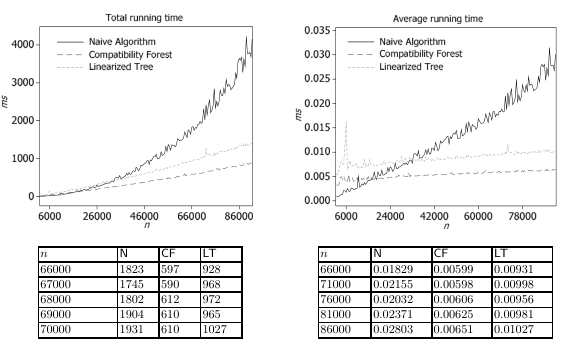
The experiment shows that the difference of total running time between algorithms undergoing a sequence of operations with number of insertion less then 6000 is small, especially between and . However, when we increase the number of insert operations, performs much slower than two other algorithms. The average running time per operation of is increasing similarly to a linear function, whereas the average running time per operation of and increases much slower. The experiment also shows that updates the interval set with low sparsity faster than .
Experiments 2 and 3. In the next two experiments we measure the performance of and undergoing a sequence of operations with the equal number of insert and query operations. We excluded from the experiments because performs too slowly when the number of query operations increases. The difference between the second and the third experiment is in the number of remove operations. Sequences in Experiment 2 do not contain remove operations. Sequences in Experiment 3 contain remove operations. We set the sparsity parameter to be . Figure 7 shows the results of Experiment 2, Figure 8 shows the results of Experiment 3.
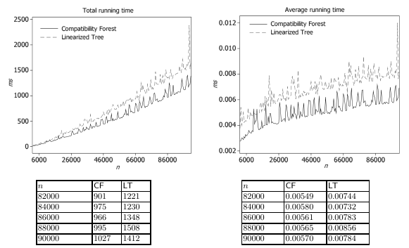
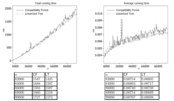
The third experiment shows that if we do not allow remove operations, performs faster than . If we allow remove operations, performs slightly slower than . However, the results of Experiment 2 show that if the interval set is not sparse, inserts and removes intervals faster than .
Conclusion. The experimental result verifies our theoretical analysis and shows that both and runs significantly faster than the naive algorithm. Moreover, the results show that in a random environment performs as fast as to within a constant factor, despite the worst () time upper bound. Considering that is relatively easy to implement, can find its practical applications.
References
- [1] D. Corneil. A simple 3-sweep LBFS algorithm for the recognition of unit interval graphs. Discrete Applied Mathematics, 2004, 138(3), 371-379.
- [2] X. Deng, P. Hell and J. Huang. Linear-time representation algorithms for proper circular-arc graphs and proper interval graphs. SIAM Journal on Computing, 1996, 25(2), 390-403.
- [3] S. Fung, C. Poon, and F. Zheng. Online interval scheduling: Randomized and Multiprocessor cases. Proceedings of COCOON, 176-186, 2007.
- [4] M.J. Katz, F. Nielsen and M. Segal. Maintenance of a piercing set for intervals with applications. Algorithmica, 36(1), 2003, 59-73
- [5] R. Lipton and A. Tompkins. Online interval scheduling. Proceedings of the Fifth Annual ACM-SIAM Symposium on Discrete Algorithms, 1994, 302-311.
- [6] P. Heggernes, D. Meister, and C. Papadopoulos. A new representation of proper interval graphs with an application to clique-width. Electronic Notes in Discrete Mathematics, 2009, 32, 27-34.
- [7] H. Kaplan,E. Molad and R. Tarjan. Dynamic rectangular intersection with priorities. Proceedings of the thirty-fifth annual ACM symposium on Theory of computing, 2003, June, 639-648.
- [8] J. Kleinberg and E. Tardos. Algorithm Design, 2006.
- [9] A. Kolen, J.K. Lenstra, C.H. Papadimitriou, and F.C. Spieksma. Interval scheduling: A survey, Naval Research Logistics, 54, 5, 2007, 530–543.
- [10] Mehlhorn, K. Data structures and algorithms, Volume 3: Multi-dimensional Searching and Computational Geometry. Springer-Verlag, Berlin, 1984.
- [11] D. Sleator and R. Tarjan. A Data Structure for Dynamic Trees, Journal of computer and system sciences, 26, 3, 1983, 362–391.
- [12] D. Sleator and R. Tarjan. Self-adjusting binary search trees, Journal of the ACM, 32, 3, 1985, 652–686.