Reduced Hamiltonian for Electronic States of Dilute Nitride Semiconductors

First, we briefly review the procedure to calculate electronic states of bulk GaAs within the empirical pseudopotential method [17] to be used as the basis in the following calculations.

Hamiltonian of bulk GaAs is given by a summation of kinetic energy and atomic potential energy $V({\bm{r}})$ as

with

where $V_{\rm Ga}\,(V_{\rm As})$ is atomic pseudopotential of Ga (As) located in a unit cell specified by a lattice vector of the zinc blende structure ${\bm{R}}_{i}$. $\bm{\tau}=(a/4,a/4,a/4)$ with $a$ the lattice constant is a vector which specifies position of Ga within a unit cell. Based on the empirical point of view, we regard that Coulomb interaction between electrons, exchange and correlation interactions, etc. are effectively included in the atomic pseudopotentials. We neglected the spin-orbit interaction. First, we calculate a Hamiltonian matrix

using plane wave basis functions

with $\bm{k}$ a wavevector, $\bm{G}_{i}$ a reciprocal lattice vector, and $\Omega$ the system volume, respectively. By diagonalizing the Hamiltonian matrix, we can calculate a band energy

and a wavefunction

where $c_{n,\bm{k}+\bm{G}_{i}}$ is an eigenvector with an index $n$ specifying band. The superscript “0”indicates non-perturbed quantities. In Figure 1, we show dispersion curves of bulk GaAs evaluated using empirical pseudopotential,[17] where zero of the energy axis is set to the conduction band edge.

Using the bulk wavefunctions, we carry out perturbation calculations to evaluate energies of GaNAs. In what follows, we consider only the lowest conduction band plotted by crosses because we are interested in behavior of the conduction band edge labeled by $\Gamma_{1}$ in Fig. 1. From now on, we thus omit the index $n$ which specifies band.

Let us consider an $N\times N\times N$ supercell in which one of As atoms therein is replaced by a nitrogen atom. Although it is possible to apply the present theory for a system containing many nitrogen atoms, in this paper, we treat only the case of a single nitrogen atom. This supercell contains $4N^{3}$ primitive cells of the zinc blende structure.

Introduction of an N atom gives rise to change in crystalline potential. We take three factors into account: (i) change of the atomic potential from As to N, (ii) displacement of Ga atoms neighboring to the N atom, and (iii) displacement of As atoms at the second neighboring positions to the N atom. Then, the perturbation Hamiltonian is written as

In the right hand side of eq. (7), the first term denotes potential change from that of As to N located at the position ${\bm{R}}_{I}$. The second and the third terms are arising from displacement of atoms neighboring to the nitrogen where $\bm{\xi}_{j}$ and $\bm{\eta}_{j}$ are the displacement of the first neighboring Ga and the second neighboring As, respectively. The indices $j$ and $j^{\prime}$ run through so that ${\bm{R}}_{j}-{\bm{\tau}}+{\bm{\xi}}_{j}$ and ${\bm{R}}_{j^{\prime}}+{\bm{\eta}}_{j^{\prime}}$ indicate the positions of the first neighboring four Ga atoms and the second neighboring twelve As atoms, respectively. We set ${\bm{\xi}}_{j}$ so that the Ga atoms approach to the N atom by 0.38 Å. Similarly, ${\bm{\eta}}_{j^{\prime}}$ was determined so that the second neighboring As atoms approach to the N by 0.1 Å. These values of atom displacements were determined from total energies evaluated by the first principle calculations using CASTEP package.

We calculated matrix elements of the perturbation Hamiltonian between the Bloch states of bulk GaAs taking the three factors (i), (ii), and (iii) mentioned above into account. In Fig. 2, we plot absolute value of the matrix elements

for $\bm{k}^{\prime}=\Gamma$ as a function of $\bm{k}$. $\Omega_{uc}=a^{3}/4$ is the zinc blende unit cell volume. On the left column, $|{\cal H^{\prime}}_{\Gamma,\bm{k}}|$s are plotted on the $k_{z}=0$ plane which contains the $\Gamma$ and X-points. On the right column, $|{\cal H^{\prime}}_{\Gamma,\bm{k}}|$s on the $k_{z}=\pi/a$ plane (the L-point is included) are shown. Note that different scales are used for figures in the left and right columns and that the values are in unit of eV. From top to bottom, total value, contribution from the factor (i), and contribution from the factor (ii) are plotted, respectively. We do not show contribution from the factor (iii) the position shift of second neighboring As, since this is much smaller than others. We note that the matrix elements are basically negative values, although we plot absolute values since they are complex quantities. We see that $|{\cal H^{\prime}}_{\Gamma,\bm{k}}|$ takes a large value when $\bm{k}$ is X and L. We also see that the effect of displacement of neighboring Ga atoms is larger than that of the N potential.

Fig. 3 shows the quantity, $|{\cal H^{\prime}}_{\Gamma,\bm{k}}|^{2}/|\varepsilon^{0}_{\Gamma}-\varepsilon^{0}_{\bm{k}}|$ plotted as a function of $\bm{k}$. Similar to Fig. 2, total value, contribution from nitrogen potential, and displacement of Ga atoms are plotted from top to bottom. It is seen that $|{\cal H^{\prime}}_{\Gamma,\bm{k}}|^{2}/|\varepsilon^{0}_{\Gamma}-\varepsilon^{0}_{\bm{k}}|$ is largest when $\bm{k}$ is the L-state, although the matrix element for the X-state is larger than that for the L-state. This is because energy difference between the L and $\Gamma$, $|\varepsilon^{0}_{\Gamma}-\varepsilon^{0}_{L}|$, is smaller than $|\varepsilon^{0}_{\Gamma}-\varepsilon^{0}_{X}|$. We also see that the N potential gives rise to mixing between the $\Gamma$-state and states in vicinity of $\Gamma$, whereas displacement of Ga atoms gives rise to the intervalley mixing. These results indicates that mixing between the $\Gamma$ and L-states and/or between the $\Gamma$ and X-states is relevant to the band gap reduction.

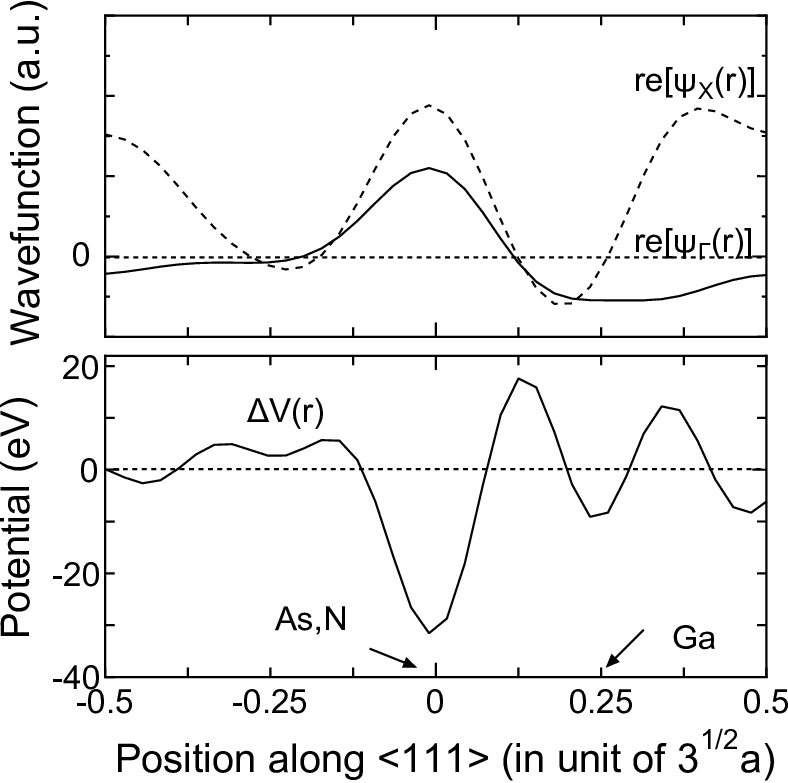
We can discern the $\bm{k}$-dependence of the perturbation matrix elements from wavefunctions of bulk GaAs. In the upper panel of Fig. 4, the solid and dashed curves show $\psi^{0}_{\Gamma}(\bm{r})$ and $\psi^{0}_{X}(\bm{r})$ plotted along the $\langle 111\rangle$ direction. The As (or N) atom locates at the position $0.0$, and a Ga atom without displacement locates at $+0.25$ as indicated by arrows. It is seen that the $\Gamma$-state wavefunction consists of anti-bonding coupling between an $s$-like orbital of As and an $s$-like orbital of Ga. We also observe that the wavefunction around Ga is largely extended. The X-state consists of anti-bonding coupling between $s$-like orbital of As and $p$-like orbital of Ga which has a node at the Ga position. The L-state has character similar to the X-state though it is not shown in the figure.

In the lower panel, we plot perturbation potential along the $\langle 111\rangle$ direction. We observe that the N atom gives rise to negative potential with $s$-like symmetry. On the other hand, perturbation potential around the Ga position is anti-symmetric around the Ga, that is, $p$-like symmetry.

These curves of crystalline potential and wavefunctions enable us to make qualitative interpretation on the matrix elements shown in the previous section. First, we consider the diagonal element ${\cal H^{\prime}}_{\Gamma,\Gamma}$ This quantity is arising mainly from N potential because $\psi^{0}_{\Gamma}$ has a large amplitude at the N position. On the other hand, shift of Ga contribute little to ${\cal H^{\prime}}_{\Gamma,\Gamma}$. This is because $\psi^{0}_{\Gamma}$ has $s$-like character around Ga. As we have noted, potential change due to Ga displacement is of $p$-character. Integration $|\psi^{0}_{\Gamma}|^{2}\times\varDelta V$around the Ga atom will make the matrix element small. The coupling between $\Gamma$ and L is also determined in the similar mechanism.

For the coupling between the $\Gamma$- and X-states ${\cal H^{\prime}}_{\Gamma,X}$, shift of Ga atoms has an important role. From Fig. 4, we see that $\psi^{0}_{\Gamma}$ has $s$-like symmetry around the Ga atom, whereas both $\psi^{0}_{X}$ and $\cal H^{\prime}$have $p$-like symmetry. Therefore, we anticipate that multiplication of these three quantities becomes even function around Ga, which enlarges the matrix element ${\cal H^{\prime}}_{\Gamma,X}$.

We noted that contribution from shift of the second neighboring As atoms is small. This is also understood from symmetry. Although displacement of As atoms is about 1/3 of that of Ga atoms, contribution might be large because of larger number (12) of neighboring As atoms. As we have noted, atom’s position change gives rise to perturbation potential with $p$-like symmetry. As seen from Fig. 4, both the $\Gamma$-state and X-state have $s$-like charge distribution around As atoms. From a simple consideration on symmetry, we see that $\langle\psi^{0}_{\bm{k}}|{\cal H^{\prime}}|\psi^{0}_{\bm{k}^{\prime}}\rangle$ with $\bm{k}$ and $\bm{k}^{\prime}$ $\Gamma$ or X has a small value.

These results indicates that mixing between $\Gamma$ and X or between $\Gamma$ and L induced by lattice distortion around N gives rise to band gap reduction of GaNAs.

The matrix elements of the perturbation Hamiltonian for a single N atom in an $N\times N\times N$ supercell are written as

where $1/{4N^{3}}$ is a factor to be normalized over the supercell. The states $\bm{k}$ and $\bm{k}^{\prime}$ at which ${\cal H^{\prime}}_{\bm{k},\bm{k}^{\prime}}^{(N)}$ is evaluated are obtained as follows: Since the perturbation potential has translational symmetry with a period $Na$ in all the $x$-, $y$-, and $z$-directions, $\langle\psi^{0}_{\bm{k}}|{\cal H^{\prime}}|\psi^{0}_{\bm{k}^{\prime}}\rangle$ must be unchanged when ${\cal H^{\prime}}({\bm{r}})$ is replaced by ${\cal H^{\prime}}({\bm{r}+\bm{R}})$ with a lattice vector of the supercell $\bm{R}$. From this, the wavevectors $\bm{k}$ and $\bm{k}^{\prime}$ in eq. (9) must satisfy a relation

with $n_{x},n_{y}$, and $n_{z}$ integers. In Figs. 5 (a) and (b), the dots indicate possible $\bm{k}-\bm{k}^{\prime}$ plotted on the first Brillouin zone of the zinc blende structure for $N=4$ and $N=8$, respectively. Note that some points on the border are equivalent. For example, $2\pi/a(1,0,0)$ and $2\pi/a(-1,0,0)$ are identical and thus one of them must be excluded, though both are plotted in the figure. Excluding such equivalent points, we have $4N^{3}$ $\bm{k}$-points in the first Brillouin zone to be mixed due to the perturbation potential; there are 256 points for $N=4$ and 2048 points for $N=8$ necessary for calculations. We also note that these $\bm{k}$-points are the points that are folded onto the $\Gamma$-point in the Brillouin zone of the $N\times N\times N$ supercell. We can calculate conduction band energy from ${\cal H^{\prime}}_{\bm{k},\bm{k}^{\prime}}^{(N)}$ given by eq. (9) with bulk GaAs states shown in Fig. 5.

We may evaluate energy of the conduction band edge $\varepsilon_{\Gamma}$ using the matrix elements by perturbation expansion. Up to the second order term, the energy change is given by

where $x=1/4N^{3}$ is nitrogen concentration. As we show in Fig. 6 by dashed curve, the second order perturbation is insufficient to explain experimental results, indicating that higher order perturbation energies are necessary since the potential change due to nitrogen is far from moderate.

Then, in order to evaluate energy of conduction band edge, we diagonalized a matrix

Results are shown in Fig. 6 by filled circles. For comparison, we plot theoretical data from Ref. [6] by crosses. We also plot a result of supercell calculation with cutoff energy 3.0 Ryd. We see that the present perturbation calculations yield reasonable results.

References

- [1] M. Kondow, K. Uomi and T. Nozue, Jpn. J. Appl. Phys. 33, L1056 (1994).
- [2] M. Weyers, M. Sato and H. Ando, Jpn. J. Appl. Phys. 31, L853 (1992).
- [3] W. G. Bi and C. W. Tu, Appl. Phys. Lett. 70, 1608 (1997).
- [4] C. Skierbiszewski, S .P. Lepkowski, P. Perlin, T. Suski, W. Jantsch, and J. Geisz, Physica E 13 1078 (2002).
- [5] W. Shan, W. Walukiewicz, K. M. Yu, and J. W. Ager III, E. E. Haller, J. F. Geisz, D. J. Friedman, J. M. Olson, and Sarah R. Kurtz, and C. Nauka, Phys. Rev. B 62, 4211 (2000).
- [6] P. H. Tan, X. D. Luo, Z. Y. Xu, Y. Zhang, A. Mascarenhas, H. P. Xin, C. W. Tu, and W. K. Ge, Phys. Rev. B 73, 205205 (2006).
- [7] K. Uesugi, N. Morooka, and I. Suemune, Appl. Phys. Lett. 74, 1254 (1999).
- [8] S. Noguchi, S. Yagi, D. Sato, Y. Hijikata, K. Onabe, S. Kuboya, and H. Yaguchi, IEEE J. Photovoltaics, 3, 1287 (2013).
- [9] K. Sumiya, M. Morifuji, Y. Oshima, and F. Ishikawa, Applied Physics Express 6 041002 (2013).
- [10] T. Fukushima, Y. Hijikata, H. Yaguchi, S. Yoshida, M. Okano, M. Yoshita, H. Akiyama, S. Kuboya, R. Katayama, K. Onabe, Physica E 42, 2529 (2010).
- [11] Chuan-Zhen Zhao, Na-Na Li, Tong Wei, Chun-Xiao Tang, and Ke-Qing Lu, Appl. Phys. Lett. 100, 142112 (2012).
- [12] W. Shan, W. Walukiewicz, J. W. Ager III, E. E. Haller, J. F. Geisz, D. J. Friedman, J. M. Olson, and S. R. Kurtz, Phys. Rev. Lett. 82, 1221 (1999).
- [13] J. Wu, W. Walukiewicz, K. M. Yu, J. W. Ager III, E. E. Haller, Y. G. Hong, H. P. Xin, and C. W. Tu, Phys. Rev. B 65, 241303 (2002).
- [14] A. Lindsay and E. P. O’Reilly, Phys. Rev. Lett. 93 196402 (2004).
- [15] E. P. O’Reilly, A. Lindsay, S. Tomić and M. Kamal-Saadi, Semicond. Sci. Technol. 17 870 (2002).
- [16] W. J. Fan, M. F. Li, and T. C. Chong, J. B. Xia, J. Appl. Phys. 79 188 (1996).
- [17] L. Bellaiche, S.-H. Wei, and A. Zunger, Appl. Phys. Lett. 70 (1997).
- [18] L. Bellaiche, S.-H. Wei, and A. Zunger Phys. Rev. B 54, 17568 (1996).
- [19] Kurt A. Mader and A. Zunger, Phys. Rev. B 50, 17393 (1994).
- [20] P. R. C. Kent and A. Zunger Phys. Rev. B, 64, 115208 (2001)
- [21] V. Timoshevskii, M. Côté, G. Gilbert, and R. Leonelli, S. Turcotte, J.-N. Beaudry, P. Desjardins, S. Larouche, L. Martinu, and R. A. Masut, Phys. Rev. B 74, 165120 (2006).
- [22] C. -K. Tan, J. Zhang, X. -H. Li, G. Liu, B. O. Tayo, and N. Tansu, J. Display Technol., 9, 272L (2013).
- [23] Pre-Olov Lödin, J. Chem. Phys. 19, 1396 (1951).
- [24] G. Burns, Introduction to group theory with applications, Academic Press, INC, New York 1977.
- [25] H. Jones, The theory of Brillouin zones and electronc states in crystals, Second, revised edition, North-Holland, Amsterdam 1977.
- [26] S. Francoeur, M. J. Seong, M. C. Hanna, J. F. Geisz, A. Mascarenhas, H. P. Xin, and C. W. Tu, Phys. Rev. B 68, 075207 (2003).