Value Function in Maximum Hands-off Control^footnoteinfo

Optimal control is widely used in recent industrial products not just for achieving the best performance but for reducing the control effort. For example, the classical LQR (Linear Quadratic Regulator) control gives a way to consider the tradeoff between performance and control-effort reduction by using weighting functions on the states and the control inputs with the $L^{2}$ norm (i.e. the energy) [1].

Recently, a novel control method, called maximum hands-off control, that maximizes the time duration in which the control is exactly zero among the admissible controls [10, 12]. An example of hands-off control is a stop-start system in automobiles, in which an automobile automatically shuts down the engine (i.e. zero control) to avoid it idling for long periods of time, and also to reduce CO or CO2 emissions as well as fuel consumption. Therefore, the hands-off control is also called as green control [11]. Also, the hands-off control is effective in hybrid/electric vehicles, railway vehicles, networked/embedded systems, to name a few [12].

Maximum hands-off control is related to sparsity, which is widely studied in compressed sensing [3]. Sparsity is also applied to control problems such as networked control [13, 8], security of control systems [4], state estimation [15], to name a few.

A mathematical difficulty in the maximum hands-off control is that the cost function, which is defined by the $L^{0}$ measure (the support length of a function), is highly nonlinear; it is discontinuous and non-convex. To solve this problem, a recent work [10, 12] has proposed to reduce the problem to an $L^{1}$ optimal control problem, and shown the equivalence between the maximum hands-off (or $L^{0}$ optimal) control and the $L^{1}$ optimal control under the assumption of normality.

Motivated by this work, we investigate the value function in the maximum hands-off control. The value function is defined as the optimal value of the cost function of the optimal control problem. It is important to show the continuity of the value function with respect to the initial state; if the value function is continuous, then the optimality property is less sensitive against uncertainties in the initial state. Also, the value function may be used as a Lyapunov function when the optimal control is adapted to model predictive control, and the continuity is necessary for the function to be a Lyapunov function [9]. Although the $L^{0}$ measure in the maximum hands-off control is discontinuous and non-convex, we prove that the value function is a continuous and strictly convex function of the initial state in the reachable set, under an assumption on the controlled plant model.

The present paper expands on our recent conference contribution [7] by rearranging the contents and incorporating analysis of convexity of the value function.

The remainder of this paper is organized as follows: In Section 2, we give mathematical preliminaries for our subsequent discussion. In Section 3, we review the problem of maximum hands-off control. Section 4 investigates the continuity of the value function in maximum hands-off control, and Section 5 discusses its convexity. Section 6 presents an example of maximum hands-off control to illustrate the properties of continuity and convexity. In Section 7, we offer concluding remarks.

This section reviews basic definitions, facts, and notation that will be used throughout the paper.

Let $n$ be a positive integer. For a vector $x\in{\mathbb{R}}^{n}$ and a scalar $\varepsilon>0$, the $\varepsilon$-neighborhood of $x$ is defined by ${\mathcal{B}}(x,\varepsilon)\triangleq\{y\in\mathbb{R}^{n}:\|y-x\|<\varepsilon\}$, where $\|\cdot\|$ denotes the Euclidean norm in ${\mathbb{R}}^{n}$. Let ${\mathcal{X}}$ be a subset of ${\mathbb{R}}^{n}$. A point $x\in{\mathcal{X}}$ is called an interior point of ${\mathcal{X}}$ if there exists $\varepsilon>0$ such that ${\mathcal{B}}(x,\varepsilon)\subset{\mathcal{X}}$. The interior of ${\mathcal{X}}$ is the set of all interior points of ${\mathcal{X}}$, and we denote the interior of ${\mathcal{X}}$ by $\mathrm{int}{\mathcal{X}}$. A set ${\mathcal{X}}$ is said to be open if ${\mathcal{X}}=\mathrm{int}{\mathcal{X}}$. For example, $\mathrm{int}{\mathcal{X}}$ is open for every subset ${\mathcal{X}}\subset\mathbb{R}^{n}$. A point $x\in\mathbb{R}^{n}$ is called an adherent point of ${\mathcal{X}}$ if ${\mathcal{B}}(x,\varepsilon)\cap{\mathcal{X}}\neq\emptyset$ for every $\varepsilon>0$, and the closure of ${\mathcal{X}}$ is the set of all adherent points of ${\mathcal{X}}$. A set ${\mathcal{X}}\subset{\mathbb{R}}^{n}$ is said to be closed if ${\mathcal{X}}=\overline{{\mathcal{X}}}$, where $\overline{{\mathcal{X}}}$ is the closure of ${\mathcal{X}}$. The boundary of ${\mathcal{X}}$ is the set of all points in the closure of ${\mathcal{X}}$, not belonging to the interior of ${\mathcal{X}}$, and we denote the boundary of ${\mathcal{X}}$ by $\partial{\mathcal{X}}$, i.e., $\partial{\mathcal{X}}=\overline{{\mathcal{X}}}-\mathrm{int}{\mathcal{X}}$, where $\mathcal{X}_{1}-\mathcal{X}_{2}$ is the set of all points which belong to the set ${\mathcal{X}}_{1}$ but not to the set ${\mathcal{X}}_{2}$. In particular, if ${\mathcal{X}}$ is closed, then $\partial{\mathcal{X}}={\mathcal{X}}-\mathrm{int}{\mathcal{X}}$, since ${\mathcal{X}}=\overline{{\mathcal{X}}}$. A set ${\mathcal{X}}\subset{\mathbb{R}}^{n}$ is said to be convex if, for any $x,y\in{\mathcal{X}}$ and any $\lambda\in[0,1]$, $(1-\lambda)x+\lambda y$ belongs to ${\mathcal{X}}$.

A real-valued function $f$ defined on $\mathbb{R}^{n}$ is said to be upper semi-continuous on $\mathbb{R}^{n}$ if for every $\alpha\in\mathbb{R}$ the set $\{x\in\mathbb{R}^{n}:f(x)<\alpha\}$ is open, and $f$ is said to be lower semi-continuous on $\mathbb{R}^{n}$ if for every $\alpha\in\mathbb{R}$ the set $\{x\in\mathbb{R}^{n}:f(x)>\alpha\}$ is open. It is known that a function $f$ is continuous on $\mathbb{R}^{n}$ if and only if it is upper and lower semi-continuous on $\mathbb{R}^{n}$; see e.g., [14, pp. 37].

A real-valued function $f$ defined on a convex set ${\mathcal{C}}\subset{\mathbb{R}^{n}}$ is said to be convex if

for all $x$, $y\in\mathcal{C}$ and all $\lambda\in(0,1)$, and $f$ is said to be strictly convex if the inequality (1) holds strictly whenever $x$ and $y$ are distinct points and $\lambda\in(0,1)$.

Let $T>0$. For a continuous-time signal $u(t)$ over a time interval $[0,T]$, we define its $L^{1}$ and $L^{\infty}$ norms respectively by

We define the support set of $u$, denoted by $\mathrm{supp}(u)$, by the closure of the set $\{t\in[0,T]:u(t)\neq 0\}$. The $L^{0}$ norm of a measurable function $u$ as the length of its support, that is, $\|u\|_{0}\triangleq m\bigl(\mathrm{supp}(u)\bigr)$, where $m$ is the Lebesgue measure on ${\mathbb{R}}$.

In this paper, we consider a linear time-invariant system represented by

where $x(t)\in{\mathbb{R}}^{n}$, $u(t)\in{\mathbb{R}}$, $A\in{\mathbb{R}}^{n\times n}$, and $B\in{\mathbb{R}}^{n\times 1}$. Throughout this paper, we assume the following:

Let $T>0$ be the final time of control. For the system (2), we call a control $u=\{u(t):t\in[0,T]\}\in L^{1}$ admissible if it steers $x(t)$ from a given initial state $x(0)=\xi\in\mathbb{R}^{n}$ to the origin at time $T$ (i.e., $x(T)=0$), and satisfies the magnitude constraint $\|u\|_{\infty}\leq 1$. We denote by ${\mathcal{U}}(\xi)$ the set of all admissible controls for an initial state $\xi\in{\mathbb{R}}^{n}$, that is,

The maximum hands-off control is the minimum $L^{0}$-norm (or the sparsest) control among the admissible control inputs. This control problem is formulated as follows.

The value function for this optimal control problem is defined as

Note that the cost function $J(u)$ can be rewritten as

where $\phi_{0}$ is the $L^{0}$ kernel function defined by

Fig. 1 shows the graph of $\phi_{0}(u)$. As shown in this figure, the kernel function $\phi_{0}(u)$ is discontinuous at $u=0$ and non-convex. However, in the following sections, we will show that the value function $V(\xi)$ in (4) is continuous and strictly convex.

In this section, we investigate the continuity of the value function $V(\xi)$ in (4).

First, we define the reachable set for the control problem (Problem 2) by

The following is a fundamental lemma of the paper:

Note that the absolute value $|u|$ in (5) is a convex approximation of $\phi_{0}(u)$ as shown in Fig. 1. Associated with $V_{1}(\xi)$, we define the following subset of ${\mathcal{R}}$ with $\alpha\geq 0$:

For the set ${\mathcal{R}}_{\alpha}$, we have another fundamental lemma.

From these lemmas, we show the continuity of the value function $V(\xi)$.

Theorem 5 leads to an important result of $L^{1}$ optimal control as follows.

Here we show the convexity of the value function $V(\xi)$. Although the kernel function $\phi_{0}(u)$ in the cost function is not convex as shown in Fig. 1, the value function $V(\xi)$ is a convex function on ${\mathcal{R}}$.

In this section, we consider a simple example with a 1-dimensional linear control system

where $a<0$ and $b\neq 0$. This system obviously satisfies Assumption 1, and let us verify the continuity and convexity of the value function $V(\xi)$ on the reachable set ${\mathcal{R}}$.

The reachable set ${\mathcal{R}}$ and the maximum hands-off control $u_{\xi}$ for an initial state $\xi\in{\mathcal{R}}$ are computed via the bang-bang principle [6, Theorem 12.1] and the minimum principle for $L^{1}$-optimal control [2, Section 6.14] as

and

where $\mathrm{sgn}(x)=x/|x|$ for $x\neq 0$ and $\mathrm{sgn}(0)=0$, and

Note that if $\xi=0$, then $u_{0}(t)=0$ for all $t\in[0,T]$. Then we have

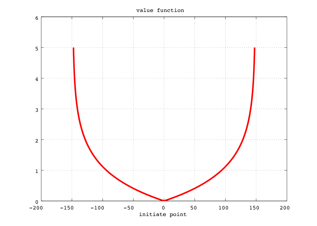
For example, let $a=-1$, $b=1$, and $T=5$. Fig. 2 shows the value function $V(\xi)$ on ${\mathcal{R}}$, where ${\mathcal{R}}=[-e^{5}+1,e^{5}-1]$. Certainly, we can see that $V(\xi)$ is continuous and strictly convex on ${\mathcal{R}}$.

In this brief paper, we have proved the continuity and the strict convexity of the value function of the maximum hands-off control problem under an assumption of the controlled system. Also, as a corollary we have shown that those properties are also satisfied for $L^{1}$ optimal control under the same assumption. These properties of the vale function plays an important role to investigate the stability when we extend the control to the model predictive control.

References

- [1] B. D. O. Anderson and J. B. Moore. Optimal Control: Linear Quadratic Methods. Dover Publications, 2007.
- [2] M. Athans and P. L. Falb. Optimal Control. Dover Publications, 1966.
- [3] Y. C. Eldar and G. Kutyniok. Compressed Sensing: Theory and Applications. Cambridge University Press, 2012.
- [4] H. Fawzi, P. Tabuada, and S. Diggavi. Secure estimation and control for cyber-physical systems under adversarial attacks. IEEE Trans. Autom. Control, 59(6):1454–1467, June 2014.
- [5] O. Hajek. -optimization in linear systems with bounded controls. Journal of Optimization Theory and Applications, 29(3):409–436, November 1979.
- [6] H. Hermes and J. P. Lasalle. Function Analysis and Time Optimal Control. Academic Press, 1969.
- [7] T. Ikeda and M. Nagahara. Continuity of the value function in sparse optimal control. submitted to the 10th Asian Control Conference 2015 (ASCC2015), 2015. http://arxiv.org/abs/1412.5707.
- [8] H. Kong, G. C. Goodwin, and M. M. Seron. A cost-effective sparse communication strategy for networked linear control systems: an SVD-based approach. International Journal of Robust and Nonlinear Control, 2014. (to appear).
- [9] M. Morari and J. H. Lee. Model predictive control: past, present and future. Computers and Chemical Engineering, 23(4-5):667–682, 1999.
- [10] M. Nagahara, D. E. Quevedo, and D. Nešić. Maximum-hands-off control and optimality. In 52nd IEEE Conference on Decision and Control (CDC), pages 3825–3830, December 2013.
- [11] M. Nagahara, D. E. Quevedo, and D. Nešić. Hands-off control as green control. In SICE Control Division Multi Symposium 2014, March 2014. http://arxiv.org/abs/1407.2377.
- [12] M. Nagahara, D. E. Quevedo, and D. Nešić. Maximum hands-off control: a paradigm of control effort minimization. 2014. http://arxiv.org/abs/1408.3025.
- [13] M. Nagahara, D.E. Quevedo, and J. Østergaard. Sparse packetized predictive control for networked control over erasure channels. IEEE Trans. Autom. Control, 59(7):1899–1905, July 2014.
- [14] W. Rudin. Real and Complex Analysis. McGraw-Hill, 3rd edition edition, 1987.
- [15] B. M. Sanandaji, M. B. Wakin, and T. L. Vincent. Observability with random observations. IEEE Trans. Autom. Control, 59(11):3002–3007, November 2014.
- [16] T. B. Singh. Elements of Topology. CRC Press, 2013.
Appendix A Proof of Lemma 4
A.1 Lemmas
To prove Lemma 4, we need some lemmas.
Lemma 8.
The set in (6) satisfies the following:
- 1.
For every , is compact.
- 2.
For every , , with equality for .
- 3.
.
- 4.
for .
PROOF.
See [5, Lemma 2.1]. ∎
Lemma 9.
For every , we have
First, fix and take any . Then, by the definition of , there exists such that and
From (3), it follows that the control is an admissible control, that is, , and also satisfies . By definition, and hence . Therefore, we have .
Lemma 10.
For each initial value , there exists an admissible control with minimal -cost . Furthermore, then, with .
See [5, Lemma 3.1]. ∎
A.2 Proof of (7)
A.3 Proof of (8) and (9)
We prove the equation (8); then the equation (9) follows immediately from (7) and (8), since is closed for every from Lemma 8. If , then , since . It follows from (7) that
Fix . We can take , since is not empty.11 1 and the empty set are the only subsets whose boundaries are empty, since is connected [16, Chapter 3]. Since , we have . If , then int (see [5, Lemma 4.2]), and hence a contradiction occurs. Therefore we have , and hence and is not empty for every . Then it follows from Lemma 10 that
for every , and the conclusion follows.