Non-euclidean shadows of classical projective theorems
![[Uncaptioned image]](1412.7589v2/crf_113_oriented_triangle.png)
§ 1 Introduction
Cayley-Klein projective models for hyperbolic and elliptic (spherical) geometries have the disadvantage of being non-conformal. However, they have some interesting virtues: geodesics are represented by straight lines, allowing to easily visualize incidence properties, and they give an unified treatment of the three classic planar geometries: euclidean, spherical and hyperbolic. They can be introduced into any course on projective geometry, and so they can give to undergraduate students an early contact with non-euclidean geometry before learning more advanced topics such as riemannian geometry or calculus in a complex variable. Within a course on projective geometry, the (extremely beautiful in itself) projective theory of conics can be enhanced by introducing Cayley-Klein models.
Almost any projective theorem about conics might have multiple interpretations as different theorems of non-euclidean geometry. For example, Chasles’ polar triangle Theorem (Theorem 4.3) asserts that a projective triangle and its polar triangle with respect to a conic are perspective: the lines joining the corresponding vertices are concurrent. This theorem has, at least, the following corollaries in non-euclidean geometry:
- •
the three altitudes of a spherical triangle are concurrent
- •
the three altitudes of a hyperbolic triangle are: (i) concurrent; or (ii) parallel (they are asymptotic through the same side); or (iii) ultraparallel (they have a common perpendicular).
- •
the common perpendiculars to opposite sides of a hyperbolic right-angled hexagon are concurrent.
Following [19] (and [18], indeed!), we say that these three results are different non-euclidean shadows of Chasles’ Theorem.


Aside from spherical and hyperbolic triangles, in the hyperbolic plane there are many other figures which verify similar trigonometric relations as the triangles do, such as Lambert and Saccheri quadrilaterals, right-angled pentagons and hexagons, etc.. Following [5], we will refer as generalized triangles to all these elliptic and hyperbolic figures which have trigonometry.
All generalized triangles are exactly the same figure when we look at them wearing “projective glasses”: in Cayley-Klein models they are the result of intersecting a projective triangle with its polar triangle with respect to the absolute conic of the model (see Figures 1.1–1.4, where right angles are denoted with the symbol ). With some general position assumptions, projective theorems involving a triangle and its polar triangle with respect to a conic will not depend on the relative position of both triangles with respect to a conic, and so they will have some different shadows as non-euclidean theorems about different generalized triangles. In this work we will explore the non-euclidean shadows of some classical theorems from planar geometry. We will adopt a classic (old-fashioned?) point of view. For more modern approaches to this subject see [19] or [24, 25], for example.
Pascal’s and Chasles’ theorems and classical triangle centers
In the previous example about Chasles’ Theorem and the concurrency of altitudes, we can see that the relation of a triangle with its polar one with respect to a conic is of key importance in the non-euclidean treatment of triangles. The set of midpoints of the sides of a triangle has a particular structure that is deduced essentially from Pascal’s Theorem, and this structure allows to prove the concurrency of medians, of side bisectors and of angle bisectors of a triangle.
Desargues’ Theorem and the non-euclidean Euler line
For an euclidean triagle, the orthocenter, the circumcenter and the barycenter are collinear. The line passing through these three points is the Euler line of the triangle, and it contains also many other interesting points such as the center of the nine-point circle. The nine-point circle is the circle passing through the midpoints of the sides of the triangle, and it contains also the feet of the altitudes of the triangle and the midpoints of the segments joining the orthocenter with the vertices of the triangle.
The Euler line and the nine-point circle have no immediate analogues in non-euclidean gometry because, in general, for a hyperbolic or elliptic triangle, the orthocenter, the circumcenter and the barycenter are non-collinear, and the midpoints of the sides and the feet of the altitudes are not concyclic. Thus, it is usually said that in non-euclidean geometry the Euler line and the nine-point circle do not exist. Nevertheless, we claim that they exist and that they are not unique. We will propose a non-euclidean version of these two objects, and a different version of them is proposed in [2]. The line that we propose as Euler line is the line which is called orthoaxis in [25]. We claim that there are enough reasons for this line to deserve the name Euler line. Giving credit to [25], we will call it Euler-Wildberger line.
Some of the classical centers of an euclidean triangle can be defined in multiple ways, all of them equivalent. However, two such definitions, equivalent under the euclidean point of view, could be non-equivalent in the non-euclidean world. We will illustrate this fact for the barycenter and the circumcenter. Using alternative definitions of these points, we will show how every non-euclidean triangle has an alternative barycenter and an alternative circumcenter, different from the standard ones. These alternative centers are collinear with the orthocenter of the triangle, and we will say that the line passing through them is the Euler-Wildberger line of the triangle. All these constructions have been introduced before in [24, 25] with a different notation. We give new proofs of them based on a reiterated application of Desargues’ Theorem.
Beyond the Euler line, we construct a nine-point conic which is a non-euclidean version of the nine-point circle.
Menelaus’ Theorem and non-euclidean trigonometry
Hyperbolic trigonometry is a recurrent topic in most treatments on non-euclidean geometry since the early works of N. I. Lobachevsky and J. Bolyai (see [7, 9]). Due to its connection with different topics as Riemann sufaces, low-dimensional topology or special relativity, it has been treated also from different viewpoints in more recent works such as [4, 5, 11, 22]. There exists a close connection between elliptic and hyperbolic trigonometry. Trigonometric relations between sides and angles of spherical and hyperbolic triangles look much more the same, with some replacements between sines and cosines into hyperbolic sines and cosines and vice versa.
Generalized triangles are characterized by having exactly six defining magnitudes among sides and non-right angles. The value (segment length or angular measurement) of each of these magnitudes is related with a side of or : the cross ratio of four points on this side provides the square power of a (circular or hyperbolic) trigonometric function of the corresponding magnitude.
There are four kinds of generalized triangles whose trigonometric relations are simpler than in the general case: elliptic and hyperbolic right-angled triangles (Figures 6.2(a) and 6.2(b) respectively), Lambert quadrilaterals (Figure 6.3(a)) and right-angled pentagons (Figure 6.3(b)). They appear when we force one of the non-right angles of a generalized triangle to be a right angle. For this reason, we will refer to them as generalized right-angled triangles. In §6 we show that all the trigonometric relations for generalized right-angled triangles are non-euclidean shadows of Menelaus’ Theorem.
A generalized triangle can be constructed by pasting together two generalized right-angled triangles. This decomposition allows us to deduce the trigonometric relations of generalized triangles from the trigonometric relations of the right-angled ones. Thus, the whole non-euclidean trigonometry can be deduced from Menelaus’ Theorem.


Carnot’s Theorem and… Carnot’s Theorem?
In §7 we extend the arguments applied in §6 to Menelaus’ Theorem to a theorem of Carnot on affine triangles (Theorem 7.1). We obtain that its non-euclidean shadows are the non-euclidean versions (for generalized triangles) of another classical theorem of Carnot (Theorem 7.2) for euclidean triangles!
Where do laws of cosines come from?
If the projective figure behind every generalized triangle is the same (triangle and polar triangle) and the measurements of its sides and angles are given in projective terms (cross ratios), it is natural to expect that the trigonometric relations of generalized triangles have indeed a projective basis (this viewpoint has been proposed also in [19]). In §6, Menelaus’ Theorem succeeds in providing all the trigonometric relations of right-angled figures and the law of sines for any, not necessarily right-angled, generalized triangle in a straightforward way. However, Menelaus’ Theorem fails with the law of cosines.
In §6, we introduce projective versions of the law of sines and the law of cosines of generalized triangles, but the non-euclidean trigonometric formulae that we obtain as translations of projective formulae are squared: the trigonometric functions appearing in each formula are always raised to the square power. In order to obtain the standard (unsquared) trigonometric formulae, we must proceed with an unsquaring process involving some choices of signs. The unsquaring process is straightforward for all the projective trigonometric formulae with the only exception of the law of cosines. In this sense, the projective law of cosines given in §6 is unsatisfactory, and it is natural to ask if there exists a better projective law of cosines: a formula relating cross ratios of points of a triangle and its polar triangle with respect to such that it translates in a straightforward way into the different laws of cosines for any generalized triangle.
Looking for the answer to this question, in §8 we reverse the strategy of earlier chapters. While in the rest of the book we have tried to find interesting non-euclidean theorems that can be deduced from classical projective ones, in §8 we started with some different non-euclidean results with the conviction that there must be a unique projective theorem (perhaps a non-classical one) hidden behind them. The projective formula behind all the laws of cosines is found after a detailed study of the set of midpoints of a triangle and its polar one. The midpoints allow to define a concept of “orientation” of a triangle based in purely projective techniques, and to obtain the actual, unsquared, trigonometric functions required. Although we don’t recognize any classical theorem as the essence of this projective law of cosines, in its proof we will need another classical theorem of affine geometry: Van Aubel’s Theorem on cevians11 1 The existence of this theorem was pointed out to the author by M. Avendano..
Appendix: Laguerres’s formula for rays
One of the starting points of this subject, prior to the work of Cayley [6], is Laguerre’s formula (3.3) expressing an euclidean angle in terms of the cross-ratio of four concurrent lines. As this formula uses a cross-ratio between lines, it cannot distinguish an angle from its supplement. In the appendix we propose a slight modification of Laguerre’s formula in such a way that it is valid for computing angles between rays.
In order to make the paper more self-contained, we will introduce in §2 some basics from projective geometry, and in §3 we will present Cayley-Klein models for planar hyperbolic and elliptic geometries. Apart from the notation that we introduce in them, a reader familar with this topic can skip §2 and §3.1.
Acknowledgements
I am very grateful to professors J. M. Montesinos, M. Avendano and A. M. Oller-Marcén for their interesting suggestions and comments during the writing of this manuscript.
This research has been strongly influenced by [20]. It has been partially supported by the European Social Fund and Diputación General de Aragón (Grant E15 Geometría).
§ 2 Basics of planar projective geometry.
We will asume that the reader is familiar with the basic concepts of real and complex planar projective geometry: the projective plane and its fundamental subsets (points, lines, pencils of lines, conics), and their projectivities (collineations, correlations). Nevertheless, we will review some concepts and results needed for understanding the rest of the paper. For rigurous definitions and proofs we refer to [8, 23], for example.
We consider the real projective plane standardly embedded in the complex projective plane . We consider the objects lying in , and they can be real or imaginary depending on how they intersect with . A point in is real if it lies in , and it is imaginary otherwise. A line in is real if is a real projective line, and it is imaginary otherwise. A nondegenerate conic in is real if is a nondegenerate real projective conic, and it is imaginary otherwise.
For two points in , let denote the line joining them. For two lines in , let denote the intersection point between them. For a line and a conic , let denote de set of intersection points between them. In , has one or two (perhaps imaginary) points, while in the intersection set can consist of , or real points. For a real line and a real conic , we say that is exterior, tangent or secant to if the intersection set has , or real points, respectively.
2.1 Cross ratios
Given a line and four different collinear points , their cross ratio is given by
| (2.1) |
where once we have chosen a set of nonhomogeneous coordinates in such that none of the points is at infinity. This formula does not depend on the chosen set of coordinates, and so the cross ratio is well-defined.
The cross ratio depends on the ordering of the four points . By simple computations it can be checked that it fulfills the following relations:
| (2.2a) | ||||
| (2.2b) | ||||
and for any point collinear with it is
| (2.2c) |
Proposition 2.1
The cross ratio of four different points is a number different from and .
Proof. If the four points are different, the four numbers in the right-hand side of (2.1) are different from and thus . Applying (2.2b), we have also .
Cross ratio can be defined even if some of the four points coincide, or if one of the points lies at infinity in the chosen set of coordinates. When one of the four points is the point at infinity of the line, the cross ratio coincides with a harmonic ratio of the three remaining points. For example, if is at infinity we have
| (2.3) |
The fundamental property of cross ratio is that it is invariant under the operations of projection from a point and section with a line 11 1 The invariance of cross-ratio under projection and section can be checked experimentally: (i) draw four collinear points on a blackboard; (ii) take a ruler and put it in front of you (with one eye closed!) making it coincide in your sight with the line containing the four points depicted; (iii) write down the numbers on the ruler that correspond to the four points in your sight; (iv) compute the cross-ratio of these four numbers. Repeat the experiment from another place of the classroom, with another ruler (cm., inches,…), etc. The resulting cross-ratio will be approximately the same. . Let be four points on a line , let be another line, and let be a point not incident with or . Take the lines joining the point with respectively, and take the points in given by (Figure 2.1)
Then, the following relation holds:22 2 If we take one of the four lines as the line at infinity and we apply (2.3), then (2.4) is Thales’ theorem.
| (2.4) |

Property (2.4) allows us to define the cross ratio of four concurrent lines. If are four concurrent lines and is a line not concurrent with them, by taking the points where intersects respectively we can define
An interesting property of cross ratio for real points is the following (see [23, vol. II, Theorem 17]):
Lemma 2.2
If are four points in a real line , then
For the sake of simplicity, in the projective context we will consider segments and triangles just as the subsets of the set of points of the projective plane composed by their vertices, without entering deeper discussions about separation or convexity. This will not be the same in the (non-euclidean) geometric context: segments and triangles will retrieve their usual meaning when considered in the hyperbolic or elliptic plane.
2.2 Segments
A segment is a pair of different points of the projective plane. The segment is denoted by . The points are the endpoints of the segment . Sometimes we will use the same name for a segment and for the line that contains it.
2.3 Triangles
A triangle is a set composed by three noncollinear points (the vertices of the triangle). Because they are noncollinear, in particular the three vertices of a triangle are different. The triangle is denoted by . A line joining two vertices of the triangle is a side of . The vertex and the side of a triangle are opposite to each other if . If are three nonconcurrent lines, then we denote by the triangle having as its sides.
2.4 Quadrangles
A quadrangle (see Figure 2.2) is the figure composed by four points (the vertices of the quadrangle), no three of which are collinear, and all the lines joining any two of them (the sides of the quadrangle). If the intersection point of two sides of the quadrangle is not a vertex of the quadrangle, we say that is a diagonal point of the quadrangle and that and are opposite sides to each other. A quadrangle has six sides, arranged in three pairs of opposite sides, and thus it has three diagonal points. The three diagonal points of the quadrangle are noncollinear: they are the vertices of the diagonal triangle of the quadrangle.

2.5 Poles and polars
Let be a nondegenerate conic.
The conic allows us to associate to each point of the plane a line which is called the polar line of with respect to . If does not belong to , there are two (perhaps imaginary) lines through which are tangent to . If are the two contact points with of the lines respectively, then it is (see Figure 2.3(a)). If lies on , then is the unique line tangent to through .
The map is the polarity induced by , and it is in fact a bijection: every line of the plane has a unique point such that . If is not tangent to , then is composed by two (perhaps imaginary) points . In this case, if are the two lines tangent to at respectively, the point verifies that . If is tangent to , then contains only one point , and it is . If , we say that is the pole of with respect to and we denote also .
Proposition 2.3
The polarity induced by is a correlation: a bijection between the set of points and the set of lines of the projective plane that preserves incidence. In particular, the poles of concurrent lines are collinear and the polars of collinear points are concurrent.
See [23, vol. I, p.124] for a proof of this statement.
A quadrangle is inscribed into if the four vertices of belong to . Quadrangles are important in the theory of conics due to the following theorem (see [23, vol. I, p.123]).
Theorem 2.4
The diagonal triangle of a quadrangle inscribed into is self-polar with respect to : each side is the polar of its opposite vertex with respect to . Conversely, every self-polar triangle with respect to is the diagonal triangle of a quadrangle inscribed into .
If is a real conic and is a real point, Theorem 2.4 provides an algorithm for drawing even if is interior to (the tangent lines to through are imaginary in this case, so we can’t draw them!): (i) draw two secant lines to through and take the points , and lying in and respectively; (ii) for the quadrangle with vertices , find the two diagonal points different from ; and (iii) the polar of with respect to is the line (see Figure 2.3). In order to find the pole of a line , take two points and draw their polars : the pole of is the intersection point .


2.6 Conjugate points and lines
Let be a line not tangent to . The polarity with respect to defines a conjugacy map given by
We say that is the conjugate point of in with respect to , and we denote it by (see Figure 2.4(a)). If is a point not lying on , we define the map from the pencil of lines through onto itself given by
for any line with . We say that is the conjugate line of with respect to , and we denote it by (see Figure 2.4(b)). Note that: (i) if lies on (resp. incident with is tangent to ), then it is (resp. ); and (ii) the conjugacy maps are involutive, that is: and .


Polarity and conjugacy are projective pransformations and therefore they preserve cross ratios: if is a projective line and are four points lying on it is
| (2.5) |
and if is a point and are four lines incident with it is
| (2.6) |
2.7 Harmonic sets and harmonic conjugacy
Two collinear segments and form an harmonic set if
Quadrangles are intimately related with harmonic sets: if are two diagonal points of a quadrangle , the two lines of the quadrangle not incident with or intersect the line in two points verifying . Indeed, if is the quadrangle of Figure 2.2, taking the points given by
by successive projections and sections we have
and thus by (2.2a) it is . This only could happen if , but by Proposition 2.1 it cannot be . Therefore it must be .
Given three different collinear points , the harmonic conjugate of with respect to is the unique point , also collinear with , such that . By (2.2b), if is the harmonic conjugate of with respect to , then is the harmonic conjugate of with respect to . If is the line containing all these points, the harmonic conjugacy map that leaves and fixed and maps each point of different from and to its harmonic conjugate with respect to and is an involution of that is, indeed, a projectivity. Every projective involution on a line has two (perhaps imaginary) fixed points, and it coincides with the harmonic conjugacy on the line with respect to its fixed points. In particular, if is not tangent to and are the intersection points of with , the conjugacy on with respect to coincides with harmonic conjugacy on with respect to and for any point it is
An interesting property of harmonic sets, wich will be useful later, is the following.
Lemma 2.5
Let be a projective triangle, and let and be two points on the side and on the side respectively such that
The diagonal points different from of the quadrilateral lie on and .
Proof. See Figure 2.5. Consider the point , and consider also . By considering the quadrangle we have that intersects the line at the harmonic conjugate of with respect to . That is, passes through . In the same way, using the quadrangle for example, it is proved that is collinear with and .
Consider now the point , and take . By considering the quadrangle we have that intersects the line at . A similar argument can be used to conclude that are collinear.
The points so constructed are the diagonal points different from of the quadrangle and it is .

2.8 Conics whose polarity preserves real elements
For the rest of the paper, we will consider a nondegenerate conic with respect to which the polar of a real point is always a real line33 3 The conics with this property are those that can be expressed by means of a 2nd degree equation with real coefficients.. This property is satified by all real conics and also by a set of imaginary conics. Moreover, two such conics are equivalent under the group of real projective collineations if and only if both are real or both are imaginary (see [23, vol. II, p. 186]). Through the whole paper, when we were talking about polar lines or points and conjugate lines or points, it must be understood that we are talking about polar lines or points, and conjugate lines or points with respect to .
§ 3 Cayley-Klein models for hyperbolic and elliptic planar geometries
In 1871, in his paper [15] Felix Klein presented his projective interpretation of the geometries of Euclid, Lobachevsky and Riemann and he introduced for them the names parabolic, hyperbolic and elliptic, respectively. Klein completed the study [6] just made in 1859 by Arthur Cayley by adding the geometry of Lobachevsky and studying also the three-dimensional cases (Cayley only paid attention to euclidean and spherical planar geometries). For the planar models, Klein considers the non-degenerate conic in the projective plane (the absolute conic). When is a real conic, the interior points of compose the hyperbolic plane, and when is an imaginary conic the whole compose the elliptic plane. When degenerates into a single line , then gives a model of the euclidean (parabolic) plane.
We will use the common term the plane either for the hyperbolic plane (when is a real conic) or for the elliptic plane (when is an imaginary conic). Geodesics in these models are given by the intersection with of real projective lines, and rigid motions are given by the set of real collineations that leave invariant the absolute conic.
In the hyperbolic plane, we still use expressions as “the intersection point of two lines” or “concurrent lines” in a projective sense, even if the referred point of intersection or concurrency is not interior to . A common notation in hyperbolic geometry is to call “parallel” to those lines intersecting on and “ultraparallel” to those lines intersecting outside . If are hyperbolic lines intersecting outside , then is the common perpendicular to and .
3.1 Distances and angles


For two points , let be the two intersection points of the line with . The points will be two real points if the absolute conic is real (Figure 3.1), and they will be imaginary if the absolute conic is imaginary. The non-euclidean distance between them is given by
| (3.1) |
if the absolute conic is real, and by
| (3.2) |
if the absolute conic is imaginary. The factors before the natural logarithms of the above expressions are arbitrary, and they are taken in order to make the hyperbolic and elliptic planes’ curvature equal to or respectively. In the elliptic case the total length of a line turns out to be .
For two lines such that , let be the two tangent lines to through . The lines are both imaginary because of the hypothesis (Figure 3.1). The angle between the lines at their intersection point is given in the hyperbolic and elliptic cases by the same formula
| (3.3) |
This formula is similar to the formula given in [16] for computing euclidean angles, and for this reason we will refer to it as Laguerre’s formula. Note that is an angle between lines, not an angle between rays as usual (see [12, 14, 17]). In particular, does not distinguish an angle from its supplement and it takes values between and . We’ll come back on this discussion in §8 and in the Appendix.
In our pictures, we will depict the hyperbolic plane as the interior points of an ellipse in , and the elliptic plane as a round 2-sphere of unit radius where antipodal points are identified. In this picture of the elliptic plane it is easier to visualize the pole-polar relation: lines are represented by great circles of the sphere, and the pole of a line is the pair of antipodal points representing the north and south poles when the line is chosen as the equator of the 2-sphere. This elliptic model has the virtue also of being locally isometric. In particular, angles and lengths of segments lower than are the same in the modelling sphere as in the elliptic plane.
Conjugacy of lines with respect to the absolute characterizes perpendicularity in both models (Figure 3.2, see [20, p.36]).
Proposition 3.1
The lines such that are perpendicular if and only if they are conjugate.


3.2 Midpoints of a segment
Take a segment in the projective plane whose endpoints do not lie on and such that the line is not tangent to . Let be the pole of , let be the lines joining with respectively, and let and be the intersection points with of and respectively (Figure 3.3). The points are the vertices of a quadrangle inscribed in having as a diagonal point. By Theorem 2.4, the other two diagonal points of lie in and it is . The segments and form a harmonic set and so it is .
Let be the two intersection points of with . As
the harmonic conjugacy of with respect to sends the points into the points respectively. In particular, it is , and by (2.2a) it is . By (2.2c), we have
| (3.4) |
In the same way, it can be checked that
| (3.5) |
If the points belong to , from the distance formulae (3.1) and (3.2), we have
This property suggest the following definition:
Definition 3.2
The points are the midpoints of the segment .
If , when is a real conic there is exactly one of the midpoints of the projective segment , say , lying in the hyperbolic segment bounded by and . In this case, is the geometric midpoint of the segment and is the pole of the perpendicular bisector of this segment. When is an imaginary conic, then and divide the line into two elliptic segments whose respective midpoints are and .
It is clear that the lines are the polars of respectively. As these lines are orthogonal to through the midpoints of , they are the segment bisectors or simply bisectors of . After dualizing:
Remark 3.3
The polars of the midpoints of are the angle bisectors or bisectors of .
An interesting characterization of midpoints is the following:
Lemma 3.4
Let be a line not tangent to , let , and take two points different from . If are two points of such that
then are the midpoints of .
Proof. Let be two points of such that . We have seen that the midpoints of verify also the identity . If we take the harmonic involutions and , of with fixed points and respectively, the composition fixes the points and so it must be the identity on . This implies that .
An immediate consequence of this lemma is:
Lemma 3.5
Let be two points not in such that is not tangent to . Then, the midpoints of are also the midpoints of .
Proof. Let be the intersection points of with , and let be the midpoints of . It is clear that . If we apply on the conjugacy with respect to , we get
and thus by Lemma 3.4 are the midpoints of .


The previous lemma gives an alternative way for constructing the midpoints of using polars (Figure 3.3): (i) take the polars ; (ii) take the intersection points and of and respectively with ; and (iii) the midpoints of are the diagonal points of the quadrangle different from . This is the result of applying the original construction of the midpoints to the segment .
In the general case, we will work with segments such that the line they belong to is in general position with respect to , that is, not tangent to . Nevertheless, sometimes we will talk about the midpoints of a segment whose underlying line could be tangent to . For dealing with such limit cases, we extend the concept of “midpoint” to such segments in the natural way. If in Figure 3.3 we move continuously the points in order to make tangent to while remain out of , one of the points (say ) become coincident with one of the points (say ) and with one of the points (say ) at the contact point of with (see Figure 3.4). The other midpoint will become the point and the identity remains unchanged.
Definition 3.6
Let be two points not lying on such that the line is tangent to at a point . We say that the midpoints of the segment are and the harmonic conjugate of with respect to .

Lemma 3.4 inspires the following notation. If is a point not in and is a line through not tangent to , we will say that the harmonic involution of with respect to and is the symmetry of with respect to . If we consider the symmetry with respect to acting on every line through not tangent to at once, we obtain the symmetry of with respect to , which corresponds projectively to the harmonic homology of the projective plane with center and axis .
3.3 Proyective trigonometric ratios
The points of (3.2) and the lines of (3.3) are imaginary. This is the reason why it is more usual to use another cross ratios when working with distances and angles.
Theorem 3.7
Let be two points in , and let be the line joining them. If is the hyperbolic plane, then
| (3.6) |
and if is the elliptic plane, then
| (3.7) |
Let be two projective lines such that their intersection point lies in . Then,
| (3.8) |
For proving this theorem, we need the following lemma:
Lemma 3.8
Let be a projective line not tangent to , let be the two intersection points of with , and let be two points of different from . Then
| (3.9) |
Proof. We will make a reiterated use of cross ratio identities (2.2). We have
If are the two midpoints of the segment , the symmetry sends into respectively and vice versa. So it is
and therefore
The cross ratio can be splitted as , and because of the identity , we have
which finally gives
The proof now follows from (2.2a).
Proof of Theorem 3.7. We will prove only (3.6). The identities (3.7) and (3.8) can be proved in a similar way.


| im | ||||||
|---|---|---|---|---|---|---|
| real | sec | int | int | |||
| ext | ||||||
| ext | ||||||
| int | ||||||
| ext | ext | |||||
Expresions (3.63.8) suggest the following notation. Take a segment whose endpoints don’t lie on and such that the line containing is not tangent to . We define the projective trigonometric ratios of the segment (compare [24]) as:
In the limit case when , we take
and we say that the segment is right. The segments and are complementary segments of . The identities (2.2a) and (2.2b) imply that , and do not depend on the chosen ordering of the endpoints of the segment . Proposition 3.9 below follows directly from Theorem 3.7 and from the properties (2.2a) and (2.2b) of cross ratios (see Figure 3.5).
Proposition 3.9
Depending on the type of absolute conic (real or imaginary) we are working with and, when is a real conic, on the relative positions of the endpoints of the segment with respect to (Figure 3.5), the projective trigonometric ratios , and have the non-euclidean trigonometric translations listed in Table 3.1.
In Table 3.1, im, ext, sec and int mean imaginary, exterior to , secant to and interior to , respectively.
§ 4 Pascal’s and Chasles’ theorems and classical triangle centers
We will deal with the most common triangle centers for generalized triangles: orthocenter, circumcenter, barycenter and incenter. Although they are very well-known for triangles, their projective interpretation provides equivalent centers for any generalized triangle.
4.1 Quad theorems

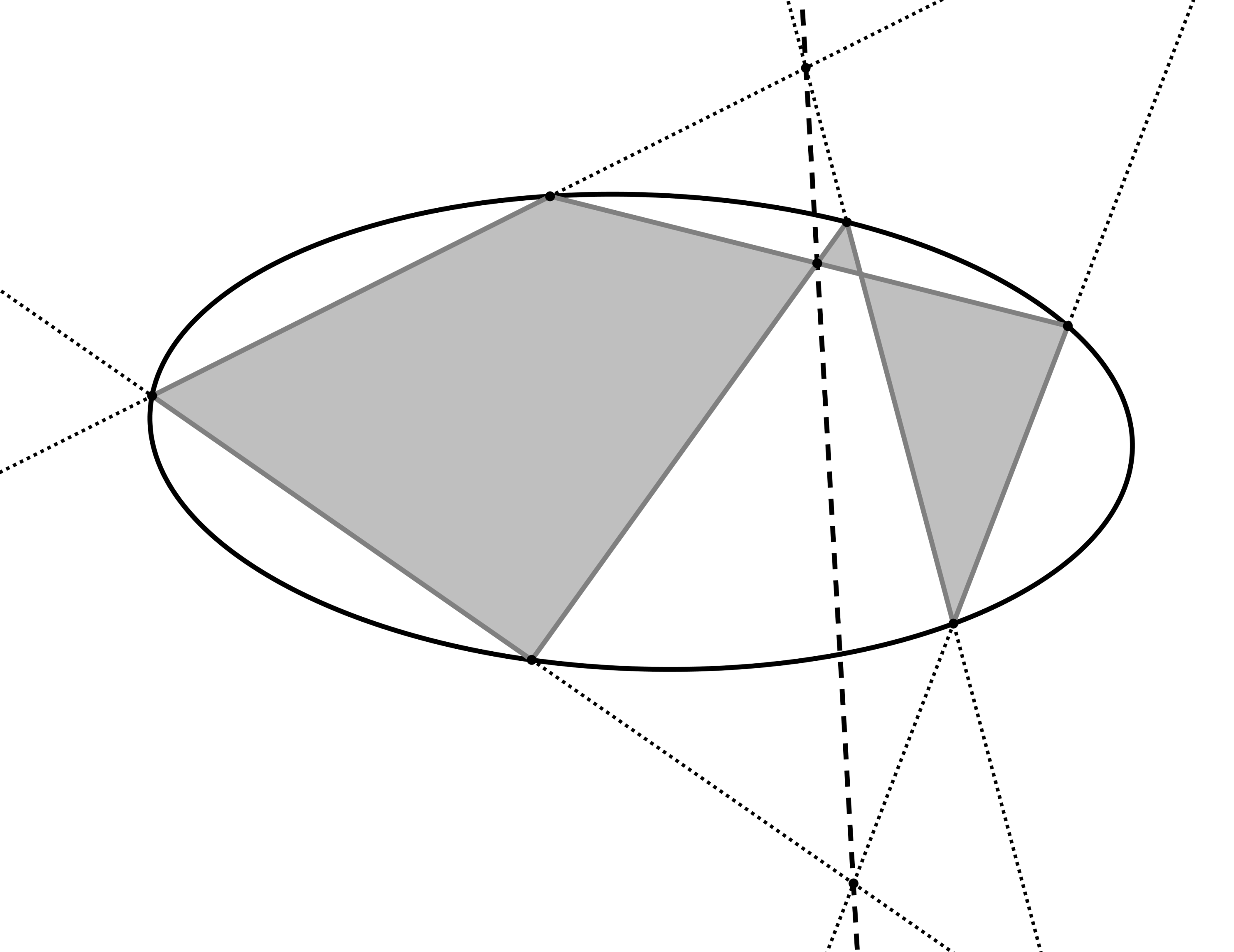
Let us state without proof four classical theorems of projective planar geometry.
Theorem 4.1 (Desargues’ Theorem)
Let and be two projective triangles. The lines are concurrent if and only if the points
are collinear.
Theorem 4.2 (Pascal’s Theorem)
If an hexagon is inscribed in a conic, the three pairs of opposite sides meet in collinear points.
Theorem 4.3 (Chasles’ polar triangle Theorem)
A triangle and its polar triangle with respect to a conic are perspective.
Theorem 4.4 (Pappus’ Involution Theorem)
The three pairs of opposite sides of a quadrangle meet any line (not through a vertex) in three pairs of an involution.
Theorem 4.4 is a partial version of Desargues’ Involution Theorem (see [8, p. 81]). Using this theorem, a given quadrangle in the projective plane determines a quadrangular involution on every line not through a vertex. If is a quadrangle, we usually denote by the quadrangular involution that it induces on the line considered. In the limit case where the line passes through a vertex of , this vertex is a double point of . For the sake of simplicity, Chasles’ polar triangle Theorem will be called “Chasles’ Theorem”.
4.2 Triangle notation
Along the whole text we will deal with a projective triangle with vertices and sides
The polar triangle of will be denoted by , its sides are the polars of respectively with respect to the absolute conic , and its vertices
are the poles of respectively. We will assume always that and are in general position: the vertices and sides of and are all different and no vertex from or lies on . This last condition implies also that no side of or is tangent to . Depending on the type of conic (real or imaginary) we are working with and, in the case of a real conic, on the relative position of the triangle with respect to the conic , the triangles and can produce in any of the generalized triangles of Figures 1.1–1.4.
Inspired by Proposition 3.1, we say that is right-angled if two of its sides are conjugate to each other. In this case, only two of its sides can be conjugate because if the sides and are both conjugate to , it turns out that is the pole of , in contradiction with the general position assumptions.
The conjugate points of the vertices of at the sides they belong to are
In the same way, the conjugate lines of the sides of are
Note that it is
The midpoints of the segments , and are , and respectively. Equivalently, the midpoints of and are denoted , and respectively.
Most of all these points and lines are depicted in Figure 4.2.

As the lines are different, among the points , there must be at least three different points. In some cases, a midpoint of and a midpoint of could coincide at the intersection point of with . We want to clarify what happens in this limit situation. Note that is also the pole of the line .
Lemma 4.5
Assume that and are both different from . If one of the points coincide with , the other one coincides too, and this happens if and only if the lines and coincide.
Proof. Assume that . This implies that the polar of passes through . The point is the conjugate point of in . Projecting the line onto since we get
By Lemmas 3.5 and 8.10 this implies that are the midpoints of .
On the other hand, if , the polar of passes through the pole of , which is and so it is , and equivalently it is .
The line is the line orthogonal to through , and therefore it is the altitude of through . In the situation of previous lemma, in the limit case when and coincide, the altitude is also a segment bisector of (as it passes through ), and an angle bisector of (as it passes through , cf. Remark 3.3). This is the reason why in this situation we say that the triangle is isosceles at . The triangle is equilateral if it is isosceles at its three vertices. As we can expect, if is isosceles at the sides incident with have the same “length”: let and be the intersection points of and with the absolute conic ; then
Proposition 4.6
The triangle is isosceles at if and only if we can label such that
| (4.1) |
Proof. If is isosceles at , the midpoint of coincides with . By §3.2, the midpoints of are the diagonal points of the quadrangle different from , so we can label such that , and (4.1) follows from projection and section since .
On the other hand, if (4.1) holds, we consider the midpoint
of . If we take the point , it turns out that
by projection and section since , and then (4.1) implies that . Therefore, belongs to , it coincides with and the triangle is isosceles at .
Proposition 4.7
If is isosceles at two vertices, it is equilateral.
As in the hypotheses of Lemma 4.5, we will always assume that and are different from . In the same way, taking the points and , we will always assume that and are different from and that and are different from . In particular, it must be , and .
4.3 Chasles’ Theorem and the orthocenter

The altitudes of through the vertices and are the lines
respectively. A straightforward consequence of Chasles’ Theorem is:
Theorem 4.8 (Concurrency of altitudes)
The lines and are concurrent.
We say that the intersection point of and is the orthocenter of . Note that the orthocenter of is also the orthocenter of .
4.4 Pascal’s Theorem and classical centers

First of all, we will introduce on the points another assumption additional to those of the last paragraph of §4.2: we will assume from now on that are non-collinear and that are non-collinear too. We show how this always can be done with the points . If is not isosceles at any vertex: (i) we take as and any of the midpoints of and respectively; (ii) as cannot be collinear with both , we choose as a midpoint of not collinear with ; and (iii) this point will be different from because is not isosceles at . If is isosceles only at : (i) we choose as the midpoint of different from ; (ii) we choose as any of the midpoints of ; and (iii) repeat steps (ii) and (iii) of the non-isosceles case. Finally, if is equilateral, we take as the midpoint of different from respectively. In this case, as are collinear it follows from Lemma 2.5 that cannot be collinear.
By Lemma 2.5, we know that and are two points on which are harmonic conjugates with respect to . In fact, these two points are .
Lemma 4.9
The points are collinear. The points are the diagonal points different from of the quadrangle .
Proof. Let , and be the intersection points of , and respectively with . By §3.2, the midpoints of are the diagonal points different from of the quadrangle . In the same way, the midpoints of are the diagonal points different from of the quadrangle , and the midpoints of are the diagonal points different from of the quadrangle .
Imagine that we have given the names , and to the points of , and respectively in such a way that
Taking the hexagon inscribed in , by Pascal’s Theorem the points are collinear with the point , which is a midpoint of (see Figure 4.4). Because we have assumed that are non-collinear, it must be .
Taking the hexagon , the points are also collinear with and therefore is a diagonal point of the quadrangle . In the same way it can be proved that is another diagonal point of .
As the polar of is the bisector of through , straightforward shadows of this lemma are (compare [20, Thm. 7]):
Theorem 4.10
Let be an elliptic or hyperbolic triangle, and let be a medial triangle of , i.e. a triangle whose vertices are midpoints of the sides of . The side bisectors of through the vertices of are the altitudes of .
Theorem 4.11
Let be a hyperbolic right-angled hexagon, and let be a triangle whose vertices are the midpoints of alternate sides of . The side bisectors of through the vertices of are the altitudes of .
The dual figure of a quadrangle is a quadrilateral: the figure composed by four lines not three of which are concurrent (the sides of the quadrilateral), and the six points at which these four lines intersect in pairs (the vertices of the quadrilateral). For any vertex of a quadrilateral there is exactly another vertex of such that the line is not a side of . We say that and are opposite vertices of and that is a diagonal line of . The three diagonal lines of compose the diagonal triangle of . A glance at Figure 2.2 gives the following result.
Lemma 4.12
Let be a quadrangle, let be a diagonal point of and let be the four sides of not passing through . Then, the vertices of the quadrilateral are the vertices of together with the two diagonal points of different from . The diagonal triangle of has as sides the sides of passing through and the side of the diagonal triangle of not passing through .
The following is an interesting property of midpoints (compare [19, Theorem 22.5]). Its proof is straightforward from Lemmas 4.9 and 4.12.
Theorem 4.13
The midpoints of the sides of are the vertices of a quadrilateral whose diagonal triangle is .
We say that is the midpoint quadrilateral of . This theorem has many important consequences as it allows to prove the concurrence of medians, the concurrence of side bisectors and (after dualizing) the concurrence of angle bisectors of generalized triangles.

Although we are interested in triangles , in general position with respect to , in some of our constructions we will need to use some accessory triangles which could not verify the general position assumptions. In particular, we wonder if Theorem 4.13 is valid for triangles with sides tangent to .
Lemma 4.14
Theorem 4.13 remains valid even if the triangle has sides tangent to .
Proof. Let assume that the side is tangent to , while and are not. Let be the point of tangency of with . The polars of respectively pass through . Let be the intersection points of with , and let be the intersection points of with respectively different from (Figure 4.5). The midpoints of are the diagonal points different from of the quadrangle , and the midpoints of are the diagonal points different from of the quadrangle . Thus, the line pass through a midpoint of and through a midpoint of , and so does the line . In other words, is a diagonal point of the quadrangle . By Definition 3.6 and Lemma 2.5 it follows that the other midpoint of is the other diagonal point of the quadrangle different from .

Let assume now that the sides are tangent to while is not. Let be the contact points of with and let be the midpoints of different from respectively. The polar of is the line . Let be the intersection points of with different from respectively (Figure 4.6). The points are the diagonal points of the quadrangle different from . Consider the points and . By Pascal’s Theorem on the degenerate hexagon the points , and are collinear. Taking the quadrangle it must be and, equivalently, . Therefore, are the diagonal points of different from .
In the two previous cases, Lemma 4.12 completes the proof.
Finally, let assume that are tangent to at the points respectively. In this case, is the polar triangle of . As and are perspective by Chasles’ Theorem, the points , , belong to the line . In particular, are the diagonal points of the quadrangle different from . This implies that , and thus is the midpoint of different from . In the same way, are the midpoints of different from respectively. The midpoints are the vertices of the quadrilateral .
Theorem 4.15 (Concurrence of medians)
The medians , and of are concurrent.
Proof. By considering the triangles and , by Theorem 4.13 the intersection points of corresponding sides are
which are collinear. The result follows from Desargues’ Theorem.
Theorem 4.16 (Concurrence of side bisectors)
The side bisectors , and of are concurrent.
Proof. The points , and are, respectively, the poles of the lines , and . Because , and are collinear, their polars are concurrent.
It is interesting to note that the side bisectors of are the angle bisectors of (cf. Remark 3.3). Thus, if are non-collinear midpoints of , respectively, we have (compare [9, 10.21]):
Corollary 4.17 (Concurrence of angle bisectors)
The angle bisectors of are concurrent.
A point where three concurrent medians of intersect is a barycenter of , a point where three concurrent side bisectors of intersect is a circumcenter of , and a point where three angle bisectors of intersect is an incenter of . Each generalized triangle has four barycenters, four circumcenters and four incenters. All these centers have different geometric interpretations depending on the relative position of the figure with respect to .

Another center, which as the orthocenter is shared by and , is given by the following result.
Theorem 4.18
The lines and are concurrent.
This theorem fits perfect for a right-angled hexagon.
Theorem 4.19
In a hyperbolic right-angled hexagon the lines joining the midpoints of opposite sides are concurrent.
In Figure 4.7 it is depicted a right-angled hexagon with the intersection point of the lines joining opposite midpoints. In the same figure, we have depicted also: three alternate medians of the hexagon, lines orthogonal to a side through the midpoint of its opposite side, and the intersection point of them; and its two circumcenters (or incenters, for this figure both concepts are the same), the points and where the orthogonal bisectors of alternate sides intersect.
In order to interpret Theorem 4.18 for elliptic or hyperbolic triangles, note that the point is the pole of a bisector of , and therefore is the line through orthogonal to . As the points are non-collinear, their polars are non-concurrent. This leads us to the shadow of Theorem 4.18 for hyperbolic or elliptic triangles.
Theorem 4.20
Let be a hyperbolic or elliptic triangle with vertices and opposite sides respectively. Let be non-collinear midpoints of respectively, and let be non-concurrent bisectors of through respectively. The lines orthogonal to through respectively are concurrent.
This theorem is true also in Euclidean geometry, where the lines orthogonal to through are in fact angle bisectors of the medial triangle of (the triangle whose vertices are the midpoints of the sides of ). The concurrency point of the angle bisectors of the medial triangle of is the Spieker center of the triangle . In the non-euclidean case, the lines , and are not necessarily bisectors of , and because of this we say that the concurrency point of , and given by Theorem 4.18 is the pseudo Spieker center of .
The pseudo Spieker center closes an interesting “concurrency graph”. Let denote by and the medial triangles and . The triangles , , and are perspective in pairs. If we codify each perspectivity between triangles as an edge joining the corresponding triangles, we obtain the complete graph of Figure 4.8.
§ 5 Desargues’ Theorem, alternative triangle centers and the Euler-Wildberger line
In §4 we have presented the most common centers of a triangle, using their standard definitions. In euclidean geometry, these points can be defined in multiple ways, all of them equivalent, but these definitions which are equivalent in euclidean geometry could be non-equivalent in the non-euclidean context. Thus, definitions that in euclidean geometry produce the same center in non-euclidean geometry produce different centers, all of them having reminiscences of their euclidean analogue. Desargues’ Theorem will allow us to construct a collection of such pseudocenters having some interesting properties.
5.1 Pseudobarycenter

The barycenter of an euclidean or non-euclidean triangle is the intersection point of the medians of the triangle. In euclidean geometry, the barycenter of a triangle is also the barycenter of its medial triangle and the barycenter of its double triangle (the triangle whose medial triangle is ). This is not true in non-euclidean geometry.
We define the double triangle of as the triangle whose sides
are the orthogonal lines to the altitudes through the vertices of respectively. Let , , be the vertices of . In euclidean geometry, the lines are parallel to respectively and the lines coincide with the medians of . This does not happen in the non-euclidean geometries, so we will call pseudomedians of to the lines .
Proposition 5.1
The pseudomedians of are concurrent.
Proof. The sides of the triangle intersect the sides of at the collinear points respectively. The result follows from Desargues’ Theorem.
We say that the point of intersection of the pseudomedians of is the pseudobarycenter of , and that the points , , where each pseudomedian of intersects its opposite side are the pseudomidpoints of (compare [2]).
Proposition 5.2
The altitudes of are orthogonal to the sides of the pseudomedial triangle .
Proof. It suffices to prove that is orthogonal to . The triangles and are perspective with perspective center . By Desargues’ Theorem, the intersection points
are collinear. This implies that . The point is the pole of , so the lines and are conjugate.
The following proposition, trivial in euclidean geometry, is Theorem 16 of [25].
Proposition 5.3
Even in the non-euclidean geometries, the points are midpoints of the sides of .
Proof. The quadrangle has and as diagonal points, and it is and . Thus, it is . As the points and are conjugate with respect to , by Lemma 3.4 and are the midpoints of the segment . The same holds for and , which are the midpoints of and respectively.
5.2 Pseudocircumcenter

Let be the orthogonal lines to through the pseudomidpoints of , respectively. We will say that are the pseudobisectors of the sides of respectively.
Proposition 5.4
The pseudobisectors of are concurrent.
Proof. By Proposition 5.2, the sides of the triangle pass through and . The result follows by applying Desargues’ Theorem to the triangles and .
We will call pseudocircumcenter to the point where the pseudobisectors intersect.
The pseudocircumcenter has other analogies with the classical circumcenter of euclidean geometry. Consider the lines
and the points
as in Figure 5.3. In euclidean geometry, the points lie on the circumcircle of , and they are the symmetric points of respectively through the circumcenter. This does not happen in general in non-euclidean geometry, but nevertheless we have:
Proposition 5.5
The lines intersect at the pseudocircumcenter .
Proof. It suffices to show that lies on .
We consider the triangles and . We have:
Because the points are collinear, by Desargues’ Theorem the triangles must be perspective. Thus, the line is concurrent with the pseudobisectors and , whose intersection point is .

The definition of the points is symmetric with respect to and , so we have also:
Proposition 5.6
The lines intersect at the pseudocircumcenter of .
The triangle has a property similar to that of Proposition 5.2 for the triangle :
Proposition 5.7
The altitudes of are orthogonal to the sides of .
Proof. The proof is also identical to that of Proposition 5.2. It suffices to prove that is orthogonal to . The triangles and are perspective with perspective center . By Desargues’ Theorem, the intersection points
are collinear. This implies that , and so the lines and are conjugate.
Another interesting property is the following:
Proposition 5.8
The points are collinear.
Proof. Take the triangles and . The lines , and concur at the point . Thus, the intersection points
are collinear.
The previous proposition has the following geometric translation:
Proposition 5.9
The lines are orthogonal to respectively.
5.3 The Euler-Wildberger line
Theorem 5.10
The orthocenter , the pseudobarycenters and of and respectively, and the pseudocircumcenters and of and respectively are collinear.

Proof. Consider the triangles and (Figure 5.4). The lines , and concur at . By Desargues’ Theorem, the intersection points
are collinear. Let be the line through . In the same way, it can be proved that and belong to a line .
Let consider now the triangles and (Figure 5.5). The lines and concur at the point . The intersection points
are collinear and so it must be .

Thus, the line joining and is a non-euclidean version of the Euler line. This is the line which is called orthoaxis in [25], and because of this we say that is the Euler-Wildberger line of . Another interesting non-euclidean version of the Euler line is the Euler-Akopyan line given in [2].
Theorem 5.11
The pseudobarycenter of is the pole of the orthic axis of .
The orthic axis of is the trilinear polar of the orthocenter with respect to the triangle . If
are the feet of the altitudes of , by Desargues’ Theorem the points
are collinear, and is the line joining them.
Proof. The polar of is the line . Hence, the polar triangle of the orthic triangle of is the double triangle of . If and are the other two sides of and
are the vertices of , then we have also
The polar line of is the line joining and . Thus, it is a pseudomedian of , and the pole of is the intersection of the pseudomedians of , which is the pseudobarycenter of .
Because passes through , we have the following corollary, which is also true in the euclidean case.
Corollary 5.12
The Euler-Wildberger line is the line orthogonal to the orthic axis of through the orthocenter .
The previous corollary can be used to define the line before introducing the pseudocenters . This is the way followed in [24].
5.4 The nine-point conic
The nine-point circle of euclidean triangle is a particular version of a more general construction from projective geometry: the eleven point conic. Let us describe briefly this object.
Let be a quadrangle in the projective plane with vertices , and let be a line not through a vertex of . Let be the six sides of , and assume that and , and , and are pairs of opposite sides of . For each , take the intersection point of with , and consider also the harmonic conjugate of with respect to the two vertices of lying on . Let be the quadrangular involution that induces in , and let be the two fixed points of .
Theorem 5.13 (The eleven-point conic)
The points, , the diagonal points of and the points lie on a conic.
Proof. See [3, vol. II, pp. 41-42]
We say that the conic given by this theorem is the eleven-point conic of the quadrangle and the line .
When is an euclidean triangle, is its orthocenter and is the line at infinity, the conic given by Theorem 5.13 is the nine-point circle of .
Let recover our projective triangle as before. By analogy with the euclidean case, we consider the cuadrangle and the line polar of the orthocenter with respect to , and we will study the eleven-point conic of and .
The diagonal points of are the feet of the altitudes of , so it is .

Let consider now the sides of . The intersection points are respectively.
Lemma 5.14
The harmonic conjugate of with respect to and is respectively.
Proof. By considering the quadrangle (Figure 5.6) and using that , it can be seen that is the harmonic conjugate of with respect to .
Thus, we have and in the same way .

Finally, consider the side of the quadrangle . Let be the intersection point of with . We need to find the harmonic conjugate of with respect to . Take the lines and , and the points and . If we take the quadrangle , we have that and are diagonal points of and thus (Figure 5.7). In a similar way, using also the line and the points , , and , we can find other two points of as in Figures 5.8 and 5.9. The lines are the perpendicular lines to the altitudes through the orthocenter, and so in euclidean geometry they are parallel to the sides of the triangle. The quadrangular involution of coincides with the conjugacy with respect to , so if is imaginary, or if is real and is interior to , the fixed points of are imaginary.

In analogy with euclidean geometry, we have
Proof. It suffices to prove that the opposite sides and of the hexagon inscribed in intersect at . If we consider the hexagon , with alternate vertices in the lines , by Pappus’ Theorem the intersection points of opposite sides
are collinear. This completes the proof.

There are some more properties of the Euler-Wildberger line and the nine-point conic that we have checked experimentally (working with a real conic in GeoGebra [13]), but for which we have no proofs. Among them:
- 1.
The midpoints of and the pole of with respect to are the vertices of a self-polar triangle with respect to and .
- 2.
The line is a simmetry axis of .
- 3.
When is an ellipse11 1 is always an ellipse if is imaginary. See [7] for a classification of conics in the hyperbolic plane., its center is a midpoint of and the orthogonal line to through the center is also a simmetry axis of .
It should be interesting to find proofs for these statements and also to find more analogies between the euclidean Euler line and nine-point circle and their noneuclidean versions proposed here or in [2].
§ 6 Menelaus’ Theorem and non-euclidean
trigonometry
The following theorem is classical Menelaus’ Theorem as it is usually stated in affine geometry.
Theorem 6.1 (Menelaus’ Theorem)
Let be a triangle in the affine plane. The points on the lines , , respectively are collinear if and only if
| (6.1) |
Identity (2.3) allows to make a projective interpretation of Menelaus’ Theorem by introducing the line at infinity as part of the figure (see [23, vol. II, pp. 89-90]): if are the points at infinity of the lines respectively, then (6.1) becomes
| (6.2) |
In this projective version of (6.1), the line at infinity can be replaced with any other line of the projective plane. Assume that are collinear, and let be the line they belong to. If we consider another line and its intersection points with , and :
by Menelaus’ Theorem it is
| (6.3) |
If we apply the identity (2.2c) to each cross ratio in (6.2), we have
and by (6.3) the previous identity turns into
| (6.4) |

We will say that the figure composed by the triangle and the two lines as above is a Menelaus configuration with triangle and transversals . In order to avoid degenerate cases, we will assume that the five lines involved in a Menelaus’ configuration are always in general position: they are all distinct and no three of them are concurrent.
Thus, we have proved the following corollary of Theorem 6.1, which will be enough for our purposes:
Corollary 6.2 (Menelaus’ Projective Formula)
6.1 Trigonometry of generalized right-angled triangles


Consider a projective triangle with vertices and its polar triangle as before. Assume from now on that is right-angled: and are conjugate to each other; and that . Thus, and . Taking the conjugate points and lines
the following relations hold


The projective figure composed by the triangles and the rest of points and lines considered above has four different geometric interpretations as generalized right-angled triangles. As the lines and are conjugate to each other, they form a right angle at the point . When is an imaginary conic (and so is the elliptic plane) is an elliptic right-angled triangle (Figure 6.2(a)). When is a real conic, the triangles and can produce three different hyperbolic polygons: (i) a right-angled hyperbolic triangle when are also interior to (Figure 6.2(b)); (ii) a Lambert quadrilateral, when one of the vertices turns out to be exterior to (Figure 6.3(a)); and (iii) a right-angled pentagon, when both vertices are considered exterior to but the line is secant to (Figure 6.3(b)). If the line is exterior to , there appears again a Lambert quadrilateral inside and this is the same as case (ii).
Our strategy for obtaining trigonometric relations for generalized right-angled triangles will follow these steps:
- 1.
Take a Menelaus’ configuration with the five lines by choosing three of the lines as the sides of the triangle and the other two lines as the transversals of the configuration.
- 2.
Apply Menelaus’ Projective Formula (6.4) in order to obtain a formula relating three cross ratios of points on the figure.
- 3.
Translate the three cross ratios of the formula just obtained into projective trigonometric ratios associated to the sides of the triangles and . We so obtain a projective trigonometric formula associated with the figure.
- 4.
For every particular generalized right-angled triangle, translate the projective trigonometric formula obtained in the previous step into a non-euclidean trigonometric formula using Table 3.1.
After the fourth step, we will obtain a squared non-euclidean trigonometric formula due to the presence of the square power in all the circular and hyperbolic trigonometric ratios of Table 3.1. As we will explain later, the subjacent unsquared trigonometric formula will be the result of removing all the square powers and choosing positive signs in the trigonometric functions of the corresponding squared formula.
By an abuse of notation, we will denote each of the segments , , , , with the name of the line that contains it.
6.1.1 Non-euclidean Pythagorean Theorems
Take the Menelaus’ configuration with triangle and transversals (Figure 6.4(a)). By Menelaus’ Projective Formula we have:
| (T1) |
If we give the names to the sides and angles of generalized right-angled triangles as in Figures 6.2 and 6.3, by Table 3.1 identity (T1) translates into:
- •
for an elliptic right-angled triangle
(6.5) - •
for a hyperbolic right-angled triangle
(6.6) - •
for a Lambert quadrilateral
(6.7) - •
for a right-angled pentagon
(6.8)
If we look for the unsquared versions of formulae , we must look at each figure separately.
In the three hyperbolic figures there is no discussion if we assume, as usual, that the length of a segment is always positive. In this case, because hyperbolic sines and cosines are positive for positive arguments, it must be
for the hyperbolic right angled triangle (this formula is known as the hyperbolic Pythagorean theorem),
for the Lambert quadrilateral, and
for the right-angled pentagon.
The elliptic case is subtler than the hyperbolic ones because can be positive or negative for . We need more geometric information for deciding which of the two unsquared versions of (6.5):
is the correct one, or if both are correct but they apply to different figures. Because elliptic segments have their length in , we will extend the usual terms for angles: acute, right and obtuse; to segments in the natural way. The proof of the following proposition is left to the reader.
Proposition 6.3 (elliptic triangles I)
In the triangle of Figure 6.2(a), the hypotenuse is obtuse if and only if exactly one of the catheti is obtuse. In particular, if the triangle has an obtuse side, it has exactly obtuse sides.
Proposition 6.3 implies that if one of the three ratios , , is negative, then exactly another one is also negative while the remaining one is positive. Therefore, the correct formula for elliptic right-angled triangles is
which is known as the spherical Pythagorean theorem.
6.1.2 More trigonometric relations


There are different Menelaus’ configurations that we can build from the five lines . If we exclude those relations that are equivalent after renaming the lines of the figure, there rest the six configurations depicted in Figure 6.4.
- •
Taking the triangle and the transversals (see Figure 6.4(b)), by Menelaus’ Projective Formula we have:
| (T2) |
- •
Taking the triangle and the transversals (Figure 6.4(c)), we arrive to:
| (T3) |
- •
Taking the triangle and transversals (Figure 6.4(d)) we obtain:
(T4) - •
Taking the triangle and transversals (Figure 6.4(e)), we arrive to:
(T5) - •
Finally, taking the triangle and transversals (Figure 6.4(f)), we get:
(T6)
It can be seen that the projective trigonometric formulae (T4), (T5) and (T6) can be deduced from (T1), (T2) and (T3).
If we apply Table 3.1 to expressions (T2) to (T6), for each general right-angled triangle we obtain a collection of squared non-euclidean trigonometric formulae associated with each figure. In order to decide which is the unsquared correct formula corresponding to each squared formula, we need to use the geometric properties of each figure. In the right-angled hyperbolic pentagon there will be no discussion because all the relevant magnitudes of the figure are segments. For right-angled hyperbolic triangles and Lambert quadrilaterals, it is enough to remark that:
Proposition 6.4
A hyperbolic right-angled triangle and a Lambert quadrilateral cannot have an obtuse angle.
Proposition 6.4 is a simple consequence of the fact that the sum of the angles of a hyperbolic triangle is lower than . For elliptic right-angled triangles, besides Proposition 6.3 it should be necessary also the properties listed in Proposition 6.5 (whose proof is left to the reader).
Proposition 6.5 (elliptic triangles II)
The right-angled triangle of Figure 6.2(a) verifies:
- •
the angles of are equal to the sides of the polar triangle and vice versa;
- •
one of the angles of is obtuse (right) if and only if its opposite side is also obtuse (right).
6.2 Trigonometry of generalized, non right-angled, triangles
Let us consider again the triangle with sides and its polar triangle with sides as in § 4.2. We assume again that is in general position with respect to and , but we will not assume now that has conjugate lines. Thus, could be an elliptic or hyperbolic triangle, or it could compose with any of the generalized triangles depicted in Figures 1.1–1.4. We will see how all the trigonometic formulae for these figures can be deduced from the results of the previous section.
Consider the line , and take the point and its conjugate point in , which is the point (see § 4). For simplifying the notation, we denote now to the points respectively. Take also the point (Figure 6.5). The line decomposes the Figure into two Menelaus’ configurations with some common lines. We will use the following segments (see Figure 6.5):

6.2.1 The general (squared) law of sines.
If we apply the identity (T2) to the projective right-angled triangles and we obtain
respectively, and so the ratios and must coincide. Repeating the process, they must coincide also with the ratio . Therefore, the following identity holds
| (6.9) |
We will call to identity (6.9) the general law of sines (compare [5, Theorem 2.6.20] and [19, Theorem 22.6]).
If we apply Table 3.1 to (6.9) for each generalized triangle, we obtain the law of sines associated to each figure. For example, for an elliptic triangle (Figure 1.1(a)), the unsquared translation of (6.9) is
while for a hyperbolic triangle (Figure 1.1(b)) we have
For example, for the hyperbolic pentagon with four right angles (Figure 1.2(c)) we obtain
6.2.2 The general (squared) law of cosines
In order to obtain a projective trigonometric formula similar to the cosine rules of generalized triangles we need the following lemma.
Lemma 6.6
The following relations hold:
| (6.10) | ||||
| (6.11) |
By applying (2.2c) twice and (2.2a) once we have:
As cross ratios are invariant under conjugacy, it is
and so we obtain
By applying (2.2c) again, we have:
Therefore
This implies:
Using (6.10), we obtain
Then,
From the proof of Lemma 6.6 it follows that (6.10) and (6.11) are valid11 1 Formula (6.11) is a projective version of the trigonometric formulae for the angle sum and . for any three points lying on a line not tangent to , independently of the figure .
If we apply (T1) to the projective right-angled triangles and , we obtain
respectively. It can be deduced
and by (6.11), we arrive to
If we apply (T4) to the triangle , we obtain that , and so we have
| (6.12) |
For a given generalized triangle, there is a great difference between the general law of sines (6.9) and the general law of cosines (6.12) when we want to obtain their unsquared non-euclidean trigonometric translations. The unsquared trigonometric translations of (6.9) depend on a simple choice of signs that can be done in an straightforward way. On the other hand, the unsquared trigonometric translations of (6.12) depend on a multiple choice of signs due to the presence of the two square roots and the square power in the right-hand side of (6.12).
Every non-euclidean generalized triangle have six laws of cosines, one based in each side of and another one based in each non-right angle of . If and are the two projective triangles, polar to each other, that produce the non-euclidean polygon , these six cosine laws are the unsquared trigonometric translations of (6.12), when the segment varies along the three sides of and the three sides of . When is a hyperbolic generalized triangle, in [5] it is shown how to obtain all the cosine rules of by taking an orientation on the elements (sides and non-right angles) of and assigning some coefficients to these elements. In our context we would like to have another projective general law of cosines different from (6.12) whose trigonometric translations are straightforward and give the cosine rules for each (hyperbolic and elliptic) generalized triangle. We’ll explore the existence of this formula in §8. In order to obtain it, it would be desirable to express in projective terms the actual (unsquared) trigonometric functions associated to the measurements of segments and angles.
Nevertheless, every generalized triangle is the result of pasting together two generalized right-angled triangles along a side (Figures 1.1–1.4). This allows us to deduce the trigonometry of all generalized triangles from the trigonometry of generalized right-angled triangles. This suffices for presenting the whole non-euclidean trigonometry as a corollary of Menelaus’ Theorem.
§ 7 Carnot’s Theorem and… Carnot’s Theorem?
There are many geometric results which are known as Carnot’s Theorem. One of them is a generalization of Menelaus’ Theorem (see Figure 7.1(a)):
Theorem 7.1 (Carnot’s Theorem on affine triangles)
Let be a triangle in the affine plane. The six points , , on the sides of lie on a conic if and only if
Another “Carnot’s Theorem” is Theorem 7.2 below.
Let be a triangle in euclidean plane with vertices and sides as usual. Let be three points on the lines respectively, and let be the perpendicular lines to through the points respectively. Let denote the euclidean lengths of the segments , respectively (see Figure 7.1(b)).
Theorem 7.2 (Carnot’s Theorem on euclidean triangles)
The lines are concurrent if and only if
This theorem can be proved by simple application of Pythagoras’ Theorem. For a proof of Theorem 7.1, see See [23, vol. II, p. 90]. We say that the points such that are concurrent are Carnot points of .
A version of Theorem 7.2 for hyperbolic triangles is stated in [10]. Another versions for different generalized triangles can be constructed using the non-euclidean versions of Pythagoras’ theorem (see §6.1.1), or its projective version (T1). What we will see in the following is that the non-euclidean shadows of (the projective version of) Theorem 7.1 are the non-euclidean versions of Theorem 7.2 for generalized triangles.


As we did with Menelaus’ Theorem in §6, we can make a projective interpretation of Theorem 7.1 by introducing the line at infinity as part of the figure. We will use the same notation as in §6. Let be four projective lines such that no three of them are concurrent. Consider the projective triangle and take the points
Then, Theorem 7.1 turns into
Theorem 7.3 (Carnot’s Theorem on projective triangles)
Six points , , on the sides of lie on a conic if and only if
Exercise 7.4
Prove Lemma 4.9 and Theorem 4.13 based in Menelaus’ and Carnot’s Theorems instead of Pascal’s Theorem.
We will use the following corollary instead of Theorem 7.3 itself.
Corollary 7.5
Let be a triangle in the projective plane, and let , , be six points on the sides of different from lying on a conic. Let , , be another three points on the sides of . If the points are collinear then
| (7.1) |
The converse of Corollary 7.5 is not true, but we have the following result instead.
Proposition 7.6
Let be a projective triangle, and let , , be six points on the sides of different from lying on a conic. Let , , be another three points on the sides of , and consider also the point . If the identity (7.1) holds, then it is (and so are collinear) or is the harmonic conjugate of with respect to .
Proof. Assume that (7.1) is true. By Theorem 7.3 we have
This relation, together with (7.1) imply that
or equivalently by (2.2)
If , because are different points, it must be , and if , then is the harmonic conjugate of with respect to .
When dealing with our projective triangle and its polar triangle with respect to as in §4.2, we have the following:
Theorem 7.7
The points lie on a conic.
Proof. The lines are, in this order, the sides of the hexagon with consecutive vertices . By Chasles’ Theorem the lines , , are concurrent, and so, by Desargues’ Theorem, the points , and are collinear. Thus, the opposite sides of the hexagon intersect at three collinear points. By the converse of Pascal’s Theorem, the six vertices of the hexagon must lie on a conic.
It can be deduced from the previous proof that this theorem holds for any pair of perspective triangles11 1 In fact, any pair of perspective triangles are polar to each other with respect to a conic (see [8, p. 65]).. When the triangle has two conjugate sides, the conic given by Theorem 7.7 is a degenerate conic (see Figure ). Theorem 7.7, together with Corollary 7.5, allows us to obtain geometric information about a non-euclidean generalized triangle when the collinear points of Corollary 7.5 are suitably chosen.
For a similar notation to that of Corollary 7.5 and Proposition 7.6, we will use now the names , , , , , for the points , , , , , , respectively. Let be three points lying on the sides of the triangle respectively, and consider the lines
and the segments
Theorem 7.8
If the lines are concurrent, the following relation holds:
| (7.2) |
Before proving Theorem 7.8, we will prove the following lemma:
Lemma 7.9
Let be a projective line not tangent to , and let be three points of not lying on . Then,
Proof.
So we have
Proof of Theorem 7.8. Let be the intersection point of the lines , and let be the polar line of . Consider also the three points:
By Theorem 7.7 and Corollary 7.5 we have that
| (7.3) |
Because , we have that
Moreover, as it is and this implies that and are conjugate to each other. In the same way, we have that are the conjugate points of in respectively. Finally, by Lemma 7.9
This completes the proof.
Due to Proposition 7.6, identity (7.2) is a necessary but not sufficient condition for the concurrency of the lines in Theorem 7.8. In order to obtain a partial converse of Theorem 7.8 we need to introduce some new notation. For any pair of points in the projective plane such the line is not tangent to , the Carnot involution on with respect to is the composition , where and are the conjugacy with respect to and the harmonic conjugacy with respect to respectively as introduced in §2. For any other point on , is the Carnot conjugate of with respect to . With the same notation as that introduced before Theorem 7.8, let denote now by the point and consider also the line and the point .
Theorem 7.10
If the identity (7.2) holds, then it is or is the Carnot conjugate of with respect to .
Proof. Let be the conjugate points of in respectively. Let be the conjugate point of in . By the proof of Theorem 7.8, it is . By Lemma 7.9, if (7.2) holds, then (7.3) also holds. By Proposition 7.6, if (7.3) holds, it is or is the harmonic conjugate of with respect to , and this implies that
or


If the vertices of the projective triangle and the points , , lie in the non-euclidean plane , then is a non-euclidean triangle and are the perpendicular lines to through respectively. Let denote also by the non-euclidean lengths in of the segments , respectively. Theorem 7.8 implies the following (Figure 7.2):
Theorem 7.11
If is the elliptic plane and the lines are concurrent, then
| (7.4) |
Theorem 7.10 shows how we can obtain three points for which the identity (7.4) holds and such that the lines are not concurrent. If this is the case, we say that the points are fake Carnot points of . This cannot happen if is a triangle in the hyperbolic plane (Figure 7.2).
Theorem 7.12
Hyperbolic triangles have no fake Carnot points: if is the hyperbolic plane, the lines are concurrent if and only if
| (7.5) |
If (7.5) holds, then (7.2) also holds by Proposition 3.9. Thus, by Theorem 7.10, we have that equals or the Carnot conjugate of with respect to , where is, as in Theorem 7.10, the orthogonal projection of into the line .
The polar triangle of divides the projective plane into four triangular regions, and one of them contains the absolute conic (see Figure 7.2). Let us call to this region. The point does not necessarily lie in , but because and are in it must lie in . This implies that also lies in , and we will see that in this case the Carnot conjugate of with respect to cannot be in . If are the intersection points of with , as it is mentioned in §2 the conjugacy involution of coincides with the harmonic conjugacy with respect to .
For any real projective line , any two different real points on divide the line into two connected subsets (segments), say and , and the harmonic conjugacy with respect to sends onto and vice versa (cf. Lemma 2.2). Therefore,
On the other hand, if does not lie in , because it is in , its conjugate lies in but outside the hyperbolic segment . Thus, is in the hyperbolic segment , and so lies outside . In any case, because and are in , it cannot be . Because belongs to , it must be and in consequence the lines are concurrent.

Finally, we will present a version of Theorem 7.2 for right-angled hyperbolic hexagons. Let be a right-angled hexagon in the hyperbolic plane with consecutive vertices . Consider three points lying on the alternate sides , , of respectively, and let be the perpendicular lines to through respectively. Let denote now the hyperbolic lengths of the segments (see Figure 7.3). If we construct the projective triangle with vertices , and , we can apply Theorem 7.8 to and the points . After translating the projective trigonometric ratios of (7.2) to our construction using Proposition 3.9, we obtain:
Theorem 7.13
If the lines are concurrent, then
§ 8 Where do laws of cosines come from?
The projective trigonometric ratios have the inconvenience of the presence of the square power in all their geometric translations (Table 3.1). In §6 we saw that they are sufficient to deal with figures whose trigonometric formulae are simple, and that they are not suitable to work with the law of cosines of a generalized non-euclidean triangle, for example. We are looking for projective expressions associated with segments or angles whose non-euclidean translation give the actual, unsquared, trigonometric ratios of the corresponding segment or angle. This can be done using the midpoints of segments as accesory points. Another construction appears in the Appendix as Formula (A.2).
8.1 Midpoints and the unsquaring of projective trigonometric ratios


Let be two points not lying on and such that the line joining them is not tangent to . Let be the two midpoints of . The symmetry of with respect to maps and into and respectively. This implies that
and so it is
Moreover,
Remark 8.1
The previous identities imply that the two square roots of are given by and .
By definition, it is . Therefore, the two square roots of are given by and , where are the two midpoints of .
If we want to compute a square root of and a square root of , we must choose a midpoint of the segment and a midpoint of the complementary segment . By Lemma 3.5, the midpoints of are also the midpoints of and the midpoints of are the midpoints of . We say that the midpoints of are the complementary midpoints of .
Definition 8.2
The segment is oriented if we have chosen for it a midpoint and a complementary midpoint as preferred midpoints. If is oriented, we define its two associated vectors and as the ordered pairs and , respectively, together with the preferred midpoints of . We define also the projective trigonometric ratios of and :
| (8.1) | ||||
where and are respectively the preferred midpoint and the preferred complementary midpoint of .
From now on, we will reserve the term projective trigonometric ratios for the functions and just defined, while the functions defined in §3 will be called squared projective trigonometric ratios.
Note that the functions and for oriented segments work as it is expected in analogy with the circular and hyperbolic cosine and sine functions, because it is:
and so works like an “even” function while behaves like an “odd” function. For a simpler notation we use the expressions instead of .


If is imaginary, the points are real points. If are the points depicted in Figure 8.1, and we choose as preferred midpoints for them the points and of the same figure, by Lemma 2.2 it is
Therefore, in this case it is and , where is the elliptic distance between and as depicted in Figure 8.1. If are the lines joining with the pole of and is the angle between and depicted in Figure 8.1, it is also and .
When is real and is exterior to , the four points are again real points. In the situation of Figure 8.1, if and are the preferred midpoints of , it is and also . Let consider again the lines joining with the pole of . Then, because the angle in this figure is an acute angle (observe that the line and its conjugate form a right angle), it must be and .
When is a real conic and is secant to , there are some possibilities depending on the relative positions of the points with respect to . In this case, the midpoints of are real points if and only if the complementary midpoints are imaginary. This will imply that for any choice of preferred midpoints for the segment , one of the projective trigonometric ratios will be real while the other is pure imaginary. If we want to translate the projective trigonometric ratios into geometric trigonometric ratios associated with a hyperbolic magnitude, we need to decide the sign (positive or negative when the number is real, positive imaginary or negative imaginary11 1 We use the terms positive imaginary and negative imaginary in the obvious way: a positive (resp. negative) imaginary number has the form , with positive (resp. negative). when the number is pure imaginary) of and . The sign of the real number among and can always be decided “visually”, without doing explicit computations, using Lemma 2.2. On the contrary, the sign of the pure imaginary number among and cannot be decided in a simple way.
If both points are interior to , the two midpoints are real points, while the two complementary midpoints are imaginary points. Thus, we have no visual way for choosing a preferred complementary midpoint. In the situation of Figure 8.2, if is the preferred midpoint of , we have and so it is , where is the hyperbolic distance between and . On the other hand, if is a complementary midpoint of , the cross ratio must be pure imaginary because by Lemma 2.2 it is
Thus, for any choice of preferred complementary midpoint it will be , and the correct sign of this equality cannot be decided without doing explicit computations.
In the same way, if both points are exterior to , for any choice of preferred midpoints it will be and , where is the hyperbolic distance between the poins and . For example, in Figure 8.2, if is the preferred midpoint of the segment it is .
If exactly one of the two points is interior to , then the midpoints of are imaginary numbers while the complementary midpoints are real. In Figure 8.2, for example, if is the preferred complementary midpoint of it is while for any choice of a preferred midpoint of it will be , where is the hyperbolic distance between and .
In our aim of obtaining a projective version of the law of cosines, we will use the functions just defined, but we have the annoying problems of dealing with imaginary midpoints, and of deciding the sign of projective trigonometric ratios when they are pure imaginary. As we will see, we can overcome these drawbacks: we will give a construction such that no imaginary midpoint needs to be explicitly constructed and such that no sign of pure imaginary projective trigonometric ratio needs to be explicitly computed.
8.2 The magic midpoints. Oriented triangles
Consider a projective triangle and its polar triangle as in §4.2. The points and are the midpoints and the complementary midpoints of , respectively. In the same way, the points and are the midpoints and the complementary midpoints of , respectively, and and are the midpoints and the complementary midpoints of , respectively. As usual, the same notation but adding an apostrophe
holds for the midpoints and complementary midpoints of .
In order to simplify notation, we say that the midpoints (complementary midpoints) of a segment whose endpoints are vertices of are midpoints (complementary midpoints) of the corresponding side of and also midpoints (complementary midpoints) of .
If we want to apply our functions to the triangles and , we need to orient each side of both triangles in the sense of Definition 8.2. It should be interesting to do so in a coherent way. For the midpoints of and it is not difficult to establish a choice criterion based on Theorem 4.13. We have assumed that are non-collinear, and this implies that are collinear. There is a big difference between chosing or as preferred midpoints. We will say that the preferred midpoints of the sides of are coherently chosen if they are not collinear, and the same for the preferred midpoints of . Thus, if we choose the midpoints and with the assumptions of §4.2 as preferred midpoints of their respective segments, they will be coherently chosen. The choice criterion is not as easy for the complementary midpoints of , because they have not the same structure as the midpoints.
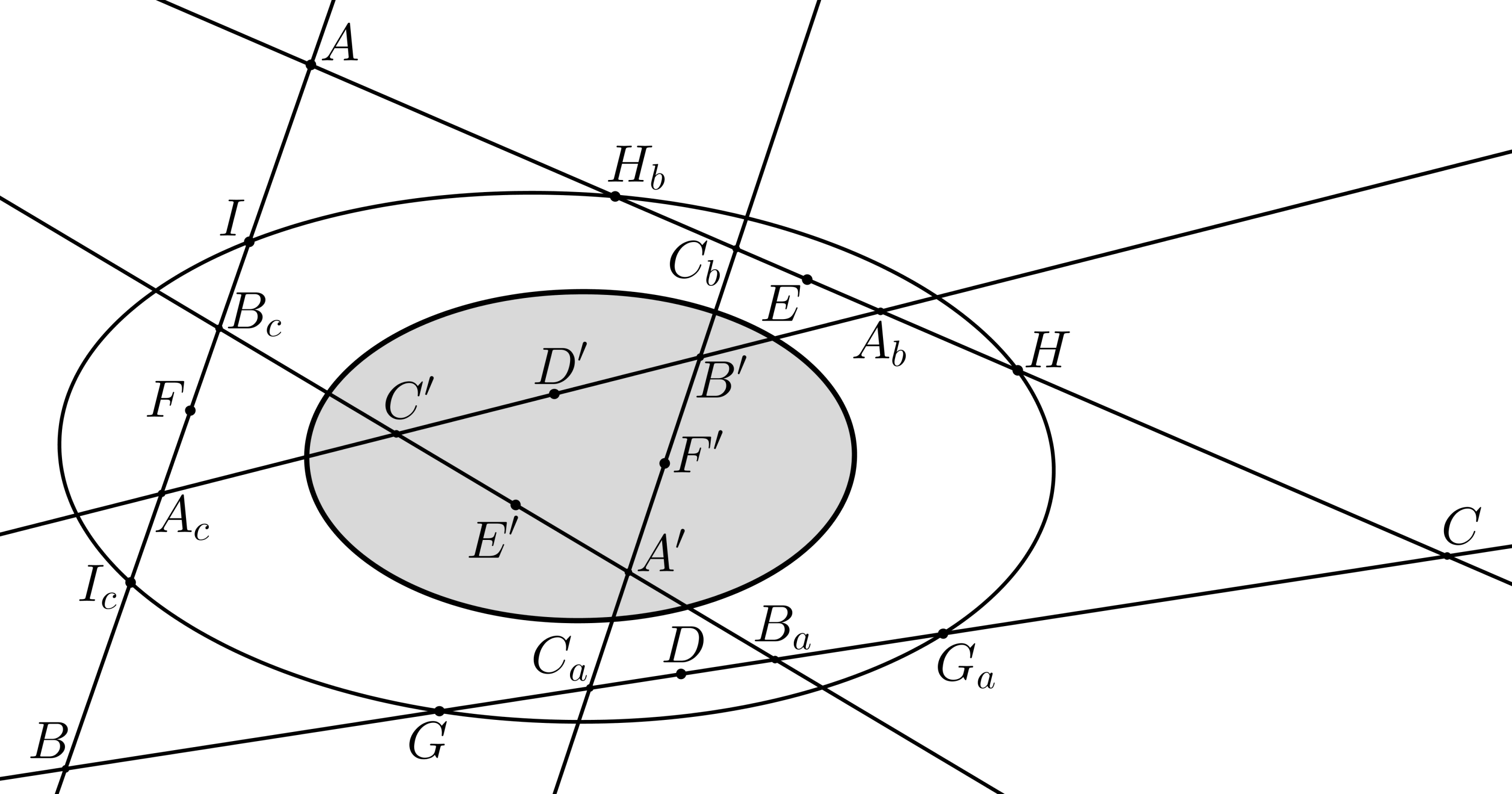
Theorem 8.3
The complementary midpoints of the triangle lie on a conic.
Before proving this theorem, we need the following lemma:
Lemma 8.4
are the midpoints of and are the midpoints of .
Proof. By Lemma 3.4, it suffices to prove that . The composition sends into respectively. Therefore, it is , and so
Proof of Theorem 8.3. Assume that the midponts of are not collinear (see Figure 8.3). Then, are collinear.
By Lemma 8.4, we have
In the same way, it is
Therefore,
The result now is a consequence of Carnot’s Theorem on projective triangles (Theorem 7.3).
Thus, until now there is no remarkable difference between choosing or as preferred complementary midpoints of . We must make a deeper exploration for finding a choice criterion for the preferred complementary midpoins of . This will need… some magic.

Let fix our sight now in the segment . Its midpoints, and the midpoints of and are very interesting because they are “in the middle of everywhere”. We need to introduce some new notation. Let be the lines respectively, let be the triangle with sides , and consider the vertices of :
The poles of are, respectively, the points
of §5. By the proof of Proposition 5.7, the lines and are concurrent, and this implies that their poles and respectively are collinear. Equivalently, is collinear with and and is collinear with and . Let be the midpoints of .
Theorem 8.5
The set coincides with:
- I
the set of intersection points ;
- II
the set of intersection points ; and
- III
the set of midpoints of .
Moreover,
- IVa
if is not isosceles at , the set coincides with the set of intersection points ;
- IVb
if is isosceles at , one of the points coincides with while the other is collinear with and .
In particular, are: (i) the diagonal points different from of the quadrangle whose vertices are the complementary midpoints of and ; (ii) the diagonal points different from of the quadrangle whose vertices are the complementary midpoints of and ; and (iii) if is not isosceles at , the diagonal points different from of the quadrangle whose vertices are the midpoints of and (Figure 8.4).
Proof. We consider the triangle . Its midpoints are the vertices of a complete quadrilateral. This proves I. An equivalent construction proves II
We prove IV before III. In order to prove IV we need:
Claim 8.5.1
The triangle is isosceles at if and only if , and are concurrent.
Proof of Claim 8.5.1. If, are concurrent, it is
Let be the perspectivity from onto with center at . Because are four different points, their cross ratio is a number different from , and so it has two different square roots which are also different from . By Remark 8.1, the two square roots of are given by and , and so the two square roots of must be given by and . This implies that the set coincides with . As we have assumed that are non-collinear and that is different from , this implies that and pass also through and so .
The previous argument can be reversed: if , the line passes through . By taking again the projection , we have that the cross-ratios and must be equal, and so their respective square powers and must be equal too. This implies that passes also through and therefore are concurrent.
Therefore, if is not isosceles at , the triangle is an actual triangle because its sides are not concurrent. In this case, we will show that the midpoints of coincide with the midpoints of the segments , , .
The vertices of the triangle are the points
Let be the midpoints of . We must prove that they are also the midpoints of the segment . The conjugate point of in is the point where the altitude of intersects the side . If we consider the quadrangle , the quadrangular involution induced by on sends the points into the points respectively and vice versa (Figure 8.5). The composition sends the points into the points , and so it coincides with the symmetry of with respect to . Then, it is
and therefore, by Lemma 3.4, the points are also the midpoints of the segment .

In the same way, it can be proved that the midpoints of are also the midpoints of , and a similar argument can be used to conclude that the midpoints of are also the midpoints of . The polar of is the line and the polar of is the line . If we consider the quadrangular involution on induced by the quadrangle , we have that sends into respectively and vice versa. The composition coincides with the symmetry of with respect to and sends into . Thus, are the midpoints of .
If is isosceles at , the lines and concur at , and the quadrangle shows that and are the midpoints of .
III. Consider the quadrangle . The quadrangular involution on sends
into
and vice versa. Thus, coincides with , and we conclude that are the midpoints of .
Remark 8.6
By Lemma 4.14, the statement of the previous theorem remains true even if is tangent to .
We will say that the triangle is the magic triangle of and that the midpoints of the sides of are the magic midpoints of . By their construction, the magic triangle and the magic midpoints of are also the magic triangle and the magic midpoints of .
Theorem 8.5 gives the key for defining a coherent orientation on a triangle in a purely projective way. The triangle is oriented if we have oriented each side of and each side of . Assume that is oriented. Following our previous notation, let and be the preferred midpoints and the preferred complementary midpoints of , respectively, and let and be the preferred midpoints and the preferred complementary midpoints of , respectively.
Definition 8.7
The triangle is coherently oriented if (see Figure 8.6)
- •
are non-collinear and different from resp.;
- •
are non-collinear and different from resp.;
and there exist non-collinear magic midpoints lying on respectively such that
- •
is the intersection point of and ;
- •
is the intersection point of and ;
- •
is the intersection point of and .
In Figure 8.6 we have depicted as an elliptic triangle. This is the only situation where midpoints, complementary midpoints and magic midpoints of and are all real points.
We will introduce some more properties about this construction. In particular, we can complete a forgotten task of our to-do list: the proof of Theorem 4.18.

Digression: the proof of Theorem 4.18
We need another classical construction from projective geometry.
Lemma 8.8
Let be two different projective lines, and let and be two tetrads of points on and on respectively such that . Then, the Pappus lines of the hexagons , , and coincide.
The proof of this Lemma is left as an exercise. A look at [8, p. 41] would help.
Remark 8.9
Assume that is coherently oriented. If and are taken as the tetrads of the previous Lemma, the resulting Pappus line is (see Figure 8.7). Similar constructions hold for and .
Proof. By Lemma 8.4, the two tetrads are harmonic sets, and so they fullfil the hypothesis of Lemma 8.8. It suffices to remember that by the chosen notation it is and .
In Figure 8.7 we can see as the Pappus line of the hexagon .

Proof of Theorem 4.18. We will divide the proof into some substeps, each of them presented as a claim.
Let consider the lines and and the points and .
Claim 8.9.1
The points are collinear (see Figure 8.8).
Proof of Claim 8.9.1. Let consider the quadrangle , and the involution that it induces on . We have that
This implies that must coincide with the symmetry on with respect to . As , it must be also .

Take the points and .
Claim 8.9.2
The points are collinear (see Figure 8.9).
Proof of Claim 8.9.2. Take the triangles and . The intersection points of corresponding sides are:
which are collinear by Claim 8.9.1. By Desargues’ Theorem, both triangles are perspective: the lines are concurrent. In other words, the line passes through .

Consider the point .
Claim 8.9.3
The points are collinear.
Proof of Claim 8.9.3. Consider the triangles and . By Remark 8.9, the point lies on and the point lies on . This implies that the intersection points of corresponding sides of both triangles are:
As we have just said, : by Desargues’ Theorem, both triangles are perspective. The lines are concurrent, but by Claim 8.9.2 the intersection point is . This completes the proof.
We can repeat step by step the proof of the previous claim but taking as starting point and considering the triangles and in order to conclude that the points are collinear, and this implies that and must coincide. This completes the proof of Theorem 4.18
End of the digression
We will use some of the notation from the proof of Theorem 4.18 in the proof of this small lemma.
Lemma 8.10
The points are the midpoints of the segment whose endpoints are and .
Proof. Consider the points and . Assume by simplicity that and are different points (the case would follow as a limit case). In the proof of Theorem 4.18 we have seen that the point is collinear with and , where is the intersection point of the lines , and . In an exactly similar way, it can be proved that is collinear with and .
Let recover the magic midpoint , and consider the quadrangle and the involution that it induces on . We have that
and that and that . Therefore,
The result now follows from Lemma 3.4.
Remark 8.11
are also the midpoints of the segment whose endpoints are and .
Remark 8.12
None of the points can be collinear with two of the points .
Definition 8.7 allows us to develop a complete trigonometry for generalized triangles. Along the next sections, we will assume that the triangle is not right-angled and that it is coherently oriented, and we will use for the preferred midpoints and complementary midpoints of and the same notation as in Definition 8.7. A good exercise would be to rewrite §6.1 using the functions in these terms.
8.3 The general law of sines
Theorem 8.13 (Projective Law of sines)
If is coherently oriented, then
| (8.2) |
Proof. Assume for instance that is the triangle depicted in Figure 8.10. If we apply Menelaus’ Projective Formula to the Menelaus’ configuration with triangle and transversals and , we obtain
where as in §8.2. Note that and that . Therefore, the previous equality is equivalent to
On the other hand if we apply Menelaus’ Projective Formula to the Menelaus’ configuration with triangle and transversals and , we obtain
where , and this last formula is equivalent to
By the proof of Theorem 8.5, if is not isosceles at we know that are the midpoints of . In this case, as are also the midpoints of , the simmetry on with respect to gives
Thus
This argument also works If is isosceles at , because in this case it is .
8.4 The general law of cosines
For proving our main result, we will need an extra help from some other classic theorems not mentioned before. After the previous chapters, a reader familiar with the classical theorems of affine and projective geometry would have the feeling that “someone’s missing”.
Theorem 8.14 (Ceva’s Theorem22 2 Although this theorem is historically attributed to the seventeenth-century italian matematician Giovanni Ceva, it is known that it was proved before by the arab mathematician Yusuf Al-Mu’taman ibn Hűd, king of Zaragoza in the eleventh century.)
We make a projective interpretation of Ceva’s Theorem exactly as we did with Menelaus’ Theorem in §6. It is usually said that Menelaus’ and Ceva’s theorems are dual to each other, but perhaps it should be said that they are harmonic to each other because harmonic conjugacy provides the equivalence between both theorems:
Lemma 8.15
Let be a projective triangle, let and be three points on the lines and respectively, and let and be their harmonic conjugates with respect to and , and and and , respectively. The lines and are concurrent if and only if the points and are collinear.
The proof of this lemma follows from Lemma 2.5, and it is left as an exercise.

We will use Ceva’s Theorem for proving another theorem, closely related to Menelaus’ and Ceva’s ones. As before, we propose a projective interpretation of the classical affine theorem.
Theorem 8.16 (Van Aubel’s Theorem on cevians)
Let be a projective triangle, and let be three points on the lines , , respectively. Let be a line not incident with , , or , and consider the points , , and (Figure 8.11). If the lines are concurrent and is their concurrence point, then
| (8.4) |
Proof. Consider the points
By Ceva’s Theorem, identity (8.3) holds. By projecting from , we have
and by projecting from we have
Ceva’s identity (8.3) implies that
By applying cross-ratio identities (2.2), we obtain
Now we are ready to state and prove our main result:
Theorem 8.17 (Projective law of cosines)
If the triangle is coherently oriented, then:
| (8.5) |
Proof.
Instead of (8.5), we will prove the equivalent dual formula
| (8.6) |
We can assume that is the triangle depicted in Figure 8.10. In that figure, is depicted as a hyperbolic triangle, and we have depicted also the polar triangle , the magic triangle , the preferred midpoints of and , the complementary midpoints of and the magic midpoints of . The figure misses the complementary midpoints of because they are imaginary.
We have that
and so
By applying Menelaus’ Projective Formula (6.4) to the Menelaus configuration with triangle and transversals and , we get
where and (Figure 8.12), and therefore

On the other hand, we have that
and so
We apply Menelaus’ Projective Formula to the Menelaus configuration with triangle and transversals and in order to obtain
where and (Figure 8.13). Therefore, it is

Finally, we have that
and then
By applying Menelaus’ Projective Formula to the Menelaus configuration with triangle and transversals and we obtain
where and (Figure 8.14). Therefore, it is

The proof of Theorem 8.17 relies now in the proof of the identity
We will need to prove some small claims before doing so.

Claim 8.17.1
The intersection point of the lines and lies on .
Proof of Claim 8.17.1. Consider the triangles and . The intersection points of the sides of both triangles are
which are collinear. By Desargues’ Theorem, the lines , and are concurrent: let be their intersection point (Figure 8.15).

The triangles and are perspective from (Figure 8.16), therefore the points , and are collinear.
Claim 8.17.2
The lines , and are concurrent. The lines , and are also concurrent. In other words, the line is a diagonal line of the quadrangle .
Proof of Claim 8.17.2. Let be the intersection point of the lines and , and consider the quadrilateral . The quadrangular involution on sends the points and into the points and respectively and vice versa, and so it coincides with . Then,
Therefore, must coincide with (Figure 8.17).
The rest of the Claim can be proved in a similar way.

It is interesting to remark that, because are midpoints of the segments respectively, the point is a midpoint of . By considering the triangle , the line must intersect at a midpoint of . Thus, it must be or .
Claim 8.17.3
The points are collinear.
Proof. Let be the line joining the points and , and take the points:
Let be the perspectivity from onto through the point , let be the perspectivity from onto through the point , and let be the perspectivity from onto through the point . Let consider also the projectivity of onto itself given by the composition .
Because the line joins the points and , it is
and so is a fixed point of .
On the other hand, looking at the midpoints of the triangle , it is
and
where is the conjugate point of in . Looking at the midpoints of the triangle , it can be
or
In the latter case, it turns out that are also fixed points of . If the point coincides with or , because it would also be or , and this is impossible by Remark 8.12. Therefore, is different from , and so the map must be the identity map on .

If we consider the point , we have
If , it should be and also , and this is not possible because is coherently oriented. Therefore, the points and are different and cannot be the identity map. Thus, it must be and .

Claim 8.17.4
The point lies in .
Proof of the Claim. By Claim 8.17.3, the line passes through . If we consider the quadrangle , the quadrilateral involution on sends into respectively and vice versa. The involution coincides with the symmetry of with respect to and it must send into . Therefore, it is .
Consider the line and the points given by
By projecting since the line onto , we have
Let consider the triangle and its cevians that intersect at . Thus, is the basepoint of the cevian through , is the basepoint of the cevian through , and is the basepoint of the cevian through . Because are collinear with and (Claims 8.17.4 and 8.17.2), the points are collinear, and therefore, by Van Aubel’s Theorem it is
This completes the proof of Theorem 8.17
8.5 Some examples
Finally, we will see that the projective laws of sines and cosines work for obtaining elliptic and hyperbolic trigonometric formulae. We show how they can be used to deduce the corresponding geometric laws for any generalized triangle. The first thing that we must do for any of of those figures is to draw the points among the midpoints, complementary midpoints and magic midpoints of and that are real points, and to label them following the requirements of Definition 8.7. We will assume always that the projective triangles depicted are coherently oriented. Then, we have to translate the projective trigonometric ratios of the projective law of cosines (8.5) into circular or hyperbolic trigonometric ratios concerning the different magnitudes of the figure. Each figure will be characterized by six geometric magnitudes that we will call . The magnitudes denote always a segment length, while or could denote an angular measure or a segment length. After that, we must deduce the sign to be put in the different terms of the geometric laws of cosines so obtained. When all the points on a cross-ratio are real points, its sign is deduced using Lemma 2.2. The main problem is to deduce the sign of a pure imaginary cross ratio (see the footnote on page 1), which appears when one of the midpoints or complementary midpoints is imaginary. We cannot deduce the sign of an imaginary without doing explicit computations. We didn’t any explicit computation in the whole book (just some tricky manipulations with cross-ratios, indeed), and we will not start now. As we will see, using only the “visible” (real) points of each figure, we can deduce the relative sign of an imaginary cross ratio of (8.5) with respect to another one. This will be done using the Projective Law of sines or using Menelaus’ Theorem together with Lemma 2.2, and it will be enough for our purposes.
8.5.1 Elliptic triangles

Let be the elliptic triangle depicted in Figure 8.20.
By applying Lemma 2.2 to the cross ratios involving the Projective Law of sines we have:
The law of sines for an elliptic triangle is:
We have also:
8.5.2 Hyperbolic triangles

Consider now the hyperbolic triangle given by in Figure 8.21. The sides and angles of have the same names as in the elliptic case. We have
From the Projective Law of sines (8.2) we deduce
In particular, , and have all the same imaginary sign: all of them are positive imaginary or all of them are negative imaginary; and the product of any two of these ratios is a negative real number.
We have, also
8.5.3 Right-angled hexagons

Consider now a right-angled hexagon with sides generated by and in the hyperbolic plane as in Figure 8.22. In this case, all the complementary midpoints of and are imaginary.
As the hyperbolic sines are always positive, the law of sines for this figure must be
Let study now the Projective Law of cosines (8.5). By Lemma 2.2, we know that the four real cross ratios of this formula: , , and are positive. This implies that the product must be negative. Otherwise, the two members of (8.5) would have different sign, which is impossible. Therefore, the law of cosines for a right-angled hexagon is
8.5.4 Quadrilateral with consecutive right angles

We study now the quadrilateral with consecutive right angles depicted in Figure 8.23. We know that
The Projective Law of sines (8.2) tells to us that and have different imaginary sign, as their quotient is a negative real number. The law of sines for this figure is
For the projective cosines, we have:
Let us start now with the dual Projective Law of cosines (8.6). The four real cross ratios of this formula: , , and are positive. This implies that the product is a negative real number, and then and have the same imaginary sign. The formula that we obtain from (8.6) is
We return now to the Projective Law of cosines (8.5). In this formula we have three unknown signs: those of , and .
We have seen by the Projective law of sines that and have different imaginary sign, and now we know also that and have the same imaginary sign. Thus, and have different imaginary sign.
On the other hand, if we apply Menelaus Projective formula to the triangle with transversals and , we get
As by Lemma 2.2, we conclude that
have the same imaginary sign. Therefore (8.5) gives
There are other two laws of cosines for this figure which are not equivalent to those given above. These are the laws of cosines given by the segments and . The first of them is
As and have the same imaginary sign, their product is a negative real number. So,
The last law of cosines we are interested in is the dual of the previous one:
All the cross-ratios involved here are real, and they give
Appendix A Laguerre’s formula for rays
As it is mentioned in §3, Laguerre’s formula (3.3) for computing angles in Cayley-Klein models is valid for angles between lines, not for angles between rays, and it cannot distinguish an angle from its supplement. We propose a modification of Laguerre’s formula that allows us to compute angles between rays. Although our formula fits perfectly in the projective model for the hyperbolic plane, it can be adapted also to the elliptic and euclidean models.
A projective conic as a 1-dimensional object is equivalent to a projective line or a pencil of lines through a point. The key for this similarity is given by Steiner’s theorem.
Theorem A.1 (Steiner’s Theorem)
Let be two points on the nondegenerate conic . The map from the pencil of lines through to the pencil of lines through that maps the line into the line for all is a projectivity.
As a corollary of Steiner’s Theorem, we obtain the following result (which is also known as “Chasles’ Theorem”):
Corollary A.2
Let be four points on the conic , and let be another two points on the same conic. If are the four lines joining the point with respectively, and are the four lines joining with respectively, then
This corollary allows us to define the cross ratio of four points on a conic as the cross ratio of the lines joining them with any other point on the conic.
Definition A.3
Given four points on the nondegenerate conic , we define their cross ratio over , and we denote it by , by the equality
where are the lines joining , respectively, with any other point of .
Assume now that is the hyperbolic plane and take a point . Consider two lines through , and take the intersection points and of and with respectively. The hyperbolic line, that we also denote by , determined by the projective line is divided by into two rays starting from and ending at respectively. In the same way, the line is divided by into the two rays starting at and ending at respectively. Let be the two tangent lines to through , and let be their contact points with , respectively. The line is the polar line of . If are the intersection points with of the lines respectively, the two diagonal points of the quadrangle different from are the midpoints of the segment . If, for example, it is , by projecting from we have
and so by (3.5) it is
This suggest the following definition:
Definition A.4
The angle between the rays is given by the formula
| (A.1) |
With this definition, angles between rays take values between and as expected. If we denote by the angle , by applying (3.9), it can be seen that
Moreover, if we draw the conjugate lines of at and we label their intersection points with as in Figure A.1 (11 1 We label the points in such a way that the lines are concurrent.), it can be proved that
| (A.2) |
Formula (A.2) shows that (A.1) works, because it gives a positive cosine for acute angles and a negative cosine for obtuse angles (cf. Lemma 2.2 for conics). If the angle between the rays is acute as in Figure A.1, the points do not separate the points . In the same figure, the angle between the rays and is obtuse because separate from , and in this case (A.2) will give a negative cosine for .
Formula (A.1) is valid for euclidean, hyperbolic and elliptic geometries if we replace the absolute conic with any circle centered at . In euclidean geometry, are Poncelet’s circular points at infinity.

Bibliography
- [2] Arseniy V. Akopyan, On some classical constructions extended to hyperbolic geometry, http://arxiv.org/abs/1105.2153
- [3] Baker, H. F., Principles of Geometry, 2nd Ed., Cambridge Universty Press 1930.
- [4] Beardon, A. F., The Geometry of Discrete Groups, New york, 1983.
- [5] Buser, P., Geometry and Spectra of Compact Riemann Surfaces, Boston, 1992.
- [6] Cayley, A., A sixth memoir upon quantics, Philosophical Transactions of the Royal Society of London, 149 (1859), pp. 61-90.
- [7] Coolidge, J. L., The elements of non-euclidean geometry, Oxford, At the Clarendon press, 1909.
- [8] Coxeter, H. S. M., The Real Projective Plane, Cambridge, 1955.
- [9] Coxeter, H. S. M., Non-euclidean geometry, Toronto, 1968.
- [10] Demirel, O. and Soytürk, E., The hyperbolic Carnot theorem in the Poincaré disc model of hyperbolic geometry, Novi Sad J. Math. 38 (2008), no. 2, 33–39.
- [11] Fenchel, W., Elementary Geometry in Hyperbolic Space, Berlin, 1989.
- [12] Forder, H. G., The cross and the foundations of euclidean geometry, Mathematical Gazette, 31 (1947), pp. 227-233.
- [13] Hohenwarter, M., GeoGebra: Ein Softwaresystem für dynamische Geometrie und Algebra der Ebene, Master Thesis, Paris Lodron University, Salzburg, Austria, 2002. Software currently developed by IGI, http://www.geogebra.org.
- [14] Johnson, Directed angles in elementary geometry, American Mathematical Monthly, 24 (1917), pp. 101-105.
- [15] Klein, F., Ueber die sogenannte Nicht-Euklidische Geometrie, Mathematische Annalen, 4 (1871), pp. 573-625. English translation in [21].
- [16] Laguerre, E., Note sur la théorie des foyers, Nouvelles Annales de Mathématiques, 12 (1853), pp. 57-66.
- [17] Picken, D. K., Euclidean geometry of angle, Proceedings of the London Mathematical Society, (2) vol. 23 (1925), pp. 45-55.
- [18] Plato, The Republic: Allegory of the Cave.
- [19] Richter-Gebert, J., Perspectives on projective geometry. A guided tour through real and complex geometry, Springer, Heidelberg, 2011.
- [20] Santaló, L., Geometrías no euclidianas, Buenos Aires, 1961.
- [21] Stillwell, J., Sources of Hyperbolic Geometry, AMS., 1996.
- [22] Thurston, W.P., Three-dimensional geometry and topology, Princeton, 1997.
- [23] Veblen and Young, Projective Geometry: vol. I, Boston, 1910; vol. II, 1918.
- [24] Wildberger, N. J., Universal hyperbolic geometry II: a pictorial overview, KoG 14 (2010), 3-24.
- [25] Wildberger, N. J., Universal hyperbolic geometry III: first steps in projective triangle geometry, KoG 15 (2011), 25-49.