(Almost) Everything You Always Wanted to Know About Deterministic Control Problems in Stratified Domains
Abstract
We revisit the pioneering work of Bressan & Hong on deterministic control problems in stratified domains, i.e. control problems for which the dynamic and the cost may have discontinuities on submanifolds of . By using slightly different methods, involving more partial differential equations arguments, we slightly improve the assumptions on the dynamic and the cost; obtain a comparison result for general semi-continuous sub and supersolutions (without any continuity assumptions on the value function nor on the sub/supersolutions); provide a general framework in which a stability result holds.
Key-words: Optimal control, discontinuous dynamic, Bellman
Equation, viscosity solutions.
AMS Class. No:
49L20, 49L25, 35F21.
1 Introduction
In a well-known pioneering work, Bressan & Hong [14] provide a rather complete study of deterministic control problems in stratified domains, i.e. control problems for which the dynamic and the cost may have discontinuities on submanifolds of . In particular, they show that the value-function satisfies some suitable Hamilton-Jacobi-Bellman (HJB) inequalities (in the viscosity solutions’ sense) and were able to prove that, under certain conditions, one has a comparison result between sub and supersolutions of these HJB equations, ensuring that the value function is the unique solution of these equations.
The aim of this article is to revisit this work by slightly improving the assumptions on the dynamic and the cost, in a (slightly) more general framework; obtaining a comparison result for general semi-continuous sub and supersolutions (while in [14] the subsolution has to be Hölder continuous, and this turns into an a priori assumption on the value function that we do not need here) ; providing a general (and to our point of view, natural) framework in which a stability result holds.
In order to be more specific, even if we are not going to enter into details in this introduction, the first key ingredient is the “stratification”, namely writing the whole space as
where, for each , is a -dimensional embedded submanifolds of , the being disjoint. The reader may consider that the are the subsets of where the dynamic and cost have discontinuities, which may also mean that, as in [14], on certain , there is a specific control problem whose dynamic and cost have nothing to do with the dynamic and cost outside . But as in our previous papers in collaboration with A. Briani dedicated to co-dimension 1 type discontinuities [6, 7], part of the dynamic and cost on is some kind of “trace” of the dynamic and cost outside . In [14], the regularity imposed on the is , while in our case it depends on the controllability of the system: is the controllable case, otherwise. This additional regularity may be seen as the price to pay for having no continuity assumption on either the value function nor the subsolutions for obtaining the equation and proving the comparison result.
The next ingredient is the control problem, i.e. the dynamic and cost. Here we are not going to enter at all into details but we just point out key facts. First, contrarily to [14], we use a general approach through differential inclusions and we do not start from dynamic and cost defined on . This may have the disadvantage to lead to a more difficult checking of the assumptions in the applications but, for example, since most of our arguments are local, the global Lipschitz assumption on the can be reduced to a locally Lipschitz one. But the most interesting feature are the controllability assumptions —and we hope to convince the reader that they are natural: for each , we assume that the system is controllable w.r.t. the normal direction(s) of in a neighborhood of each , while the dynamic and cost should also satisfy some continuity assumptions in the tangent direction(s). This controllability assumption has a clear interpretation: if, in a neighborhood of , the controller wants to go to , then he can do it, and in the same way he can avoid if this is its choice. This avoids useless discontinuities (which are not “seen” by the system) and cases where the value functions have discontinuities. We point out that this normal controllability is a key assumption to prove that the value function satisfies the right HJB inequalities without assuming a priori that it is continuous but also it is a key argument in the comparison and stability results as this was already the case in [7].
Except our slightly different approach, the viscosity sub and supersolutions inequalities are the same as in [14], even if the formulation coming from the differential inclusion and the set-valued maps for the dynamic and cost changes a litle bit the form of the Hamiltonians. The next step is more important since it concerns the comparison of any semi-continuous sub and supersolutions: here our proof differs from [14] since it involves more partial differential equations (pde for short) arguments and less control ones. A key step, already used but not in a such systematic way in [7], is to completely localize the comparison result, i.e. to reduce to the proof of comparison results in (small) balls. Once this is done, the assumptions on the allow to reduce the case when they are just affine subspaces and the key arguments of [7] can be applied (regularisation in the tangent directions to combined by a key control-pde lemma). It is worth pointing out anyway that, as in [14], the proof is done by induction on the codimension of the encountered discontinuities: local comparison in , then successively in , , …, the previous comparison result providing the key argument for the next step. We refer to the beginning of Section 5 for a more explicit exposition of the induction argument.
Finally we provide the stability result, which extends the one proved in [7] to the more complicated framework we have here but the idea remains the same: roughly speaking, the normal controllability implies that the half-relaxed limits on can be computed by using only the restrictions of the functions on , allowing to pass to the limit on the specific inequalities on (in particular for the subsolutions).
Recently, control problems in either discontinuous coefficients situations or in stratified domains or even on networks have attracted more and more attention. Of course, we start by recalling the pioneering work by Dupuis [22] who constructs a numerical method for a calculus of variation problem with discontinuous integrand. Problems with a discontinuous running cost were addressed by either Garavello and Soravia [25, 26], or Camilli and Siconolfi [17] (even in an -framework) and Soravia [38]. To the best of our knowledge, all the uniqueness results use a special structure of the discontinuities as in [20, 21, 27] or an hyperbolic approach as in [3, 19]. More in the spirit of optimal control problem on stratified domains are the ones of Barnard and Wolenski [11] (for flows invariances), Rao and Zidani [34] and Rao, Siconolfi and Zidani [35] who proved comparison results but with more restrictive controlability assumptions and without the stability results we can provide. For problems on networks which partly share the same kind of difficulties, we refer to Y. Achdou, F. Camilli, A. Cutri, N. Tchou[2], C. Imbert, R. Monneau, and H. Zidani [28], F. Camilli and D. Schieborn [15] and C. Imbert and R. Monneau [29, 30] where more and more pde methods are used, instead of control ones. A multi-dimensional version (ramified spaces) for Eikonal type equations is given F. Camilli, C. Marchi and D. Schieborn [16] and for more general equations in C. Imbert and R. Monneau [29].
We end this introduction by mentioning that this paper is focused on the specific difficulties related to stratified domains. Hence, we assume that the reader is familiar with the theory of deterministic control problems, including the approach through differential inclusions and the connections with HJB equations using viscosity solutions. Good references on this subject are [1], [4] and [24]. Let us also recall that, as was said above, we derive here a general (theoretical) framework. In a forthcoming paper we will treat several specific examples and show how the present framework applies.
The article is organized as follows: in Section 2, we describe the control problem in a full generality; this gives us the opportunity to provide all the notations and recall well-known general results which are useful in the sequel (in particular the results related to supersolutions properties). Then we have to revisit the notion of stratification and we take this opportunity to introduce the assumptions we are going to use throughout this article (Section 3). Section 4 contains the (subsolutions) properties which are specific to this context. Then we address the question of the comparison result (Section 5), reducing first to the case of the comparison in (small) balls which allows to flatten the submanifolds . Section 6 is devoted to the stability result and we conclude the article with a section collecting typical examples and extensions.
TERMINOLOGY —
| (AFS) | Admissible Flat Stratification |
| (HJB-SD) | Hamilton-Jacobi-Bellman in Stratified Domains |
| (AHG) | Assumptions on the Hamiltonian in the General case |
| (LAHF) | Local Assumptions on the Hamiltonians in the Flat case |
| (RS) | Regular Stratification |
| (TC) | Tangential Continuity |
| (NC) | Normal Controllability |
| (LP) | Lipschitz Continuity |
| Local Comparison Result in | |
| a general regular stratification of |
2 Control Problems on Stratified Domains (I):
Generalities or what is always true
In this section, we consider control problems in where the dynamics and costs may be discontinuous on the collection of submanifolds for . In this first part, we describe the approach using differential inclusions and we recall all the properties of the value-function which are always true, i.e. results where the structure of the stratification does not play any role. This is the case for all the supersolution type properties of the value function. This part is essentially expository and is kept here in order to have a self-contained article for the reader’s convenience. On the contrary, the subsolution’s properties of the value function are more specific and described in Section 4.
We first define a general control problem associated to a differential inclusion. As we mention it above, at this stage, we do not need any particular assumption concerning the structure of the stratification, nor on the control sets.
Dynamics and costs — We treat them both at the same time by embedding the cost in the differential inclusion we solve below. We denote by the set of all subsets of .
We are given a set-valued maps satisfying
-
The map has compact, convex images and is upper semi-continuous;
-
There exists , such that for any and ,
where stands for the usual euclidian norm in (which reduces to the absolute value in , for the -variable). If , corresponds to the dynamic and to the running cost, and Assumption - means that both the dynamics and running costs are uniformly bounded. In the following, we sometimes have to consider separately dynamics and running costs and to do so, we set
and analogously for .
We recall what upper semi-continuity means here: a set-valued map is upper-semi continuous at if for any open set , there exists an open set containing such that . In other terms, .
The control problem — as we said, we embed the accumulated cost in the trajectory by solving a differential inclusion in : we look for trajectories of the following inclusion
Under , it is well-known that given , there exists a Lipschitz function which is a solution of this differential inclusion. To simplify, we just use the notation when there is no ambiguity but we may also use the notations when the dependence in plays an important role. If is a solution of the differential inclusion, we have for almost any , for some . However, throughout the paper we prefer to write it this way
in order to remember that both and correspond to a specific choice in .
Then, we introduce the value function
where stands for all the Lipschitz trajectories of the differential inclusion which start at and the function is the final cost. We assume throughout the paper that is bounded and uniformly continuous.
A key standard result is the
Theorem 2.1
(Dynamic Programming Principle) Under Assumptions , the value-function satisfies
for any , .
Next we introduce the “usual” Hamiltonian for , and defined as
Using , it is easy to prove that is upper semi-continuous (w.r.t. all variables) and is convex and Lipschitz continuous as a function of only.
The second (classical) result is the
Theorem 2.2
(Supersolution’s Property) Under Assumptions , the value-function is a viscosity supersolution of
| (1) |
In Theorem 2.2, we use the classical definition of viscosity supersolution introduced by H. Ishii [31] for discontinuous Hamiltonians: we recall that a locally bounded function is a viscosity supersolution of (1) if its lower-semicontinuous envelope satifies
in the viscosity solutions’ sense, i.e. when testing with smooth function at minimum points of . Here, because of , the Hamiltonian is a locally bounded, usc function which is defined everywhere and therefore . For the sake of completeness, we recall that is a viscosity subsolution of (1) if its upper-semicontinuous envelope satifies
in the viscosity solutions’ sense, i.e. when testing with smooth function at maximum points of . But this definition of subsolution in is not the one we are going to use below.
Here and below we have chosen a formulation of viscosity solution which holds up to time , i.e. on instead of , to avoid the use of terms of the form in comparison proofs or results like [5, Lemma 2.8, p.41]
We also point out that both Theorem 2.1 and 2.2 hold in a complete general setting, independently of the stratification we may have in mind.
We conclude this first part by a converse result showing that supersolutions always satisfy a super-dynamic programming principle: again we remark that this result is independent of the possible discontinuities for the dynamic or cost.
Lemma 2.3
Let be a lsc supersolution of in . Then, for any and any ,
| (2) |
Proof — For given by , we consider the sequence of Hamiltonians
where
denoting here the distance here the set . Noticing that is Lipschitz continuous and that if , the following properties are easy to obtain
For any , and therefore is a lsc
supersolution of ,
The Hamiltonians are (globally) Lipschitz continuous w.r.t.
all variables,
as , all the other variables being
fixed.
By using and , it is clear that satisfies the Dynamic Programming Principle for the control problem associated to , namely
where solves the odes , , the controls , satisfy and the cost is
To conclude the proof, we have to let tend to . To do so, we pick an optimal or -optimal trajectory, i.e. such that
Since are uniformly bounded, standard compactness arguments imply that up to the extraction of a subsequence, we may assume that converges uniformly on to . And we may also assume that they derivatives converge in weak-* (in particular ).
We use the above property of , namely
| (3) |
in two ways: first by multiplying by , we get
But is convex in since the are convex and if converges weakly to (and converges uniformly), we have
Finally we remark that and if and only if , therefore is a solution of the -differential inclusion.
In order to conclude, we come back to (3) and we remark that since . Therefore
and we pass to the limit in this inequality using the lower-semicontinuity of , together with the weak convergence of and the uniform convergence of . This yields
and recalling that is a solution of the -differential inclusion and
taking the infimum in the left-hand side over all solution of this differential
inclusion gives the desired answer.
Q.E.D.
3 Admissible Stratifications:
how to re-read Bressan & Hong Assumptions?
In this section, we define the notion of Admissible Stratification, which specifies the structure of the discontinuity set of as was considered in [14]. We point out that, besides of the precise regularity we will impose in connection with the control problem, this notion is nothing but the notion of Whitney Stratification, based on the Whitney condition [40, 41], see below Lemma 3.2 and Remark 3.3. We first do it in the case of a flat stratification; the non-flat case is reduced to the flat one by suitable local charts.
3.1 Admissible Flat Statification
We consider here the stratification introduced in Bressan and Hong [14] but in the case when the different embedded submanifolds of are locally affine subspace of . More precisely
where the () are disjoint submanifolds of . We say that is an Admissible Flat Stratification (AFS), the following set of hypotheses is satisfied
(AFS)- For any , there exists and a -dimensional linear subspace of such that
Moreover if .
(AFS)- If for some then .
(AFS)- We have .
Remark 3.1
Condition (AFS)- implies that the set , if not void, consists of isolated points. Indeed, in the case , .
We point out that these assumptions are equivalent (for the flat case) to the assumptions of Bressan & Hong [14]. Indeed, we both assume a decomposition such that the submanifolds are disjoints and the union of all of them coincide with but in order to describe the allowed stratifications we define in a different way the submanifolds . The key point is that for us is here a -dimensional submanifold while, in [14], the can be of any dimension. In other words, our is the union of all submanifolds of dimension in the stratification of Bressan & Hong.
With this in mind it is easier to see that our assumptions (AFS)-- are equivalent to the following assumption of Bressan and Hong: if then for all indices without asking in our case. But according to the last part of (AFS)-, if : indeed for any , there exists such that . This property clearly implies (AFS)-.
In order to be more clear let us consider a stratification in induced by the upper half-plane and the -axis (see figure 1. below).
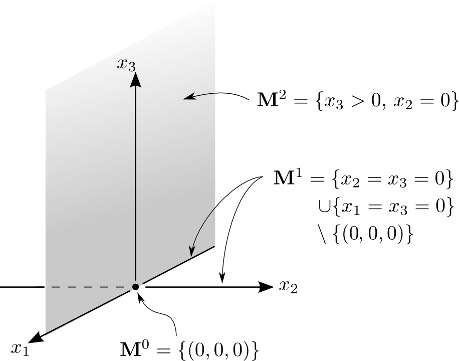
The stratification we use in this case requires first to set . The boundary of which is the -axis is included in and of course, we have to set here . Thus, consists of four connected components which are induced by the - and -axis (but excluding the origin, which is in ). Notice that in this situation, the -axis has no particular status, it is included in .
On the other hand, notice that (AFS)- FORBIDS the following decomposition of
because but clearly is not included in .
As a consequence of this definition we have following result which will be usefull in a tangential regularization procedure (see Figure 2 below)
Lemma 3.2
Let be an (AFS) of , let be in and as in (AFS)- and . Then there exists such that, if , then for any , .
Proof — We first consider the case when . We argue by contradiction assuming that there exists , . We consider the segment . There exists such that . But because of the (AFS) conditions, since no point of can be in the ball. Therefore belongs to some , a contradiction since which would imply that .
For , we argue by induction. If we have the result for , then we
use the same proof as above if : there exists , and we build in a similar way
. But this is again a
contradiction with the fact that the result holds for ; indeed and .
Q.E.D.

3.2 General Regular Stratification
Definition 3.4
We say that
is a general regular stratification (RS) of if
the following decomposition holds:
;
for any , there exists and a
-change of coordinates such that the
form an (AFS) in .
Remark 3.5
If we need to be more specific, we also say that is a stratification of , keeping the reference for the collection of changes of variable . This will be usefull in Section 6 when we consider sequences of stratifications.
Notations — The definition of regular stratifications (flat or not) allows to define, for each , the tangent space to at , denoted by , which can be identified to . Then, if and if and are as in (AFS)-, we can decompose , where is the orthogonal space to and for any we have with and . In the special case , we have , and .
At this stage, it remains to connect the stratification with the set-valued map . To do so, we first recall that the set function is said to be continuous at if when , where stands for the Haussdorf distance between sets. Now, given a regular stratification of , let us denote by the restriction of to
Definition 3.6
We say that the regular stratification of is adapted to if for any , the restriction is continuous on . In particular, the set of discontinuities of the restriction of to any is .
3.3 Hamiltonians
Considering a regular stratification adapted to , we introduce the associated Hamiltonians: if , and , the tangential Hamiltonian on the -submanifold is defined by
| (4) |
The continuity requirements on the maps (see above) together with the compactness of each implies the continuity of in , for any . In this definition (where we have implicitly identified as a subspace of ), it is clear that depends on only through its projection on but we keep the notation to simplify the notations.
Notice that in the special case , since the Hamiltonian reduces to:
In order to prove comparison for the complemented problem, we need some assumptions on the Hamiltonians that we formulate first in the case of an (AFS).
For any , if and is given by (AFS)-, there exist three constants () and a modulus of continuity with such that
(TC) Tangential Continuity: for any , for any , if with , then
We point out the importance of Lemma 3.2 which implies that this is
actually an assumption on any (or ) of .
(NC) Normal Controllability: for any , for any , if then
In particular, in the special case , we have . So, (NC) implies the coercivity w.r.t of all the Hamiltonians , , in a neighborhood of any point (recall that such points are isolated).
(LP) Lipschitz continuity: because of the boundedness of , there exists such that, for any , if then
It is worth pointing out that these assumptions (except perhaps (LP)) are local assumptions since they have to hold in a neighborrhood of each point in and the different constants or modulus of continuity may depend on the considered point. The strategy of proof for the comparison result will explain this unusual feature and in particular Lemma 5.4.
Definition 3.7
Let be a general regular stratification
associated to and be the associated Hamiltonians.
In the case of an admissible flat stratification, we
say that the associated Hamiltonians satisfy the
Local Assumptions on the Hamiltonians in the Flat case (LAHF) if
(TC), (NC) and (LP) are satisfied.
In the general case, we say that the associated Hamiltonians satisfy
the Assumption on the Hamiltonians in the general case (AHG) if the
Hamiltonians
satisfy the (LAHF), where .
In order to be complete, we give below sufficient conditions in terms of
for (TC) & (NC) to hold: the first one concerns regularity and the second one
ensures the normal coercivity of the Hamiltonians.
(TC-BL) For any , for any , if with ,
(NC-BL) There exists such that, for any , for any , if there holds
Here also, the case is particular: we impose a complete controllability of the system in a neighborhood of since the condition reduces to because .
This normal controllability assumption plays a key role in all our analysis: first, in the proof of Theorem 4.1 below, to obtain the viscosity subsolution inequalities for the value function, in the comparison proof to allow the regularization (in a suitable sense) of the subsolutions and, last but not least, for the stability result.
4 Control Problems on Stratified Domains (II):
Subsolutions and Complemented Hamilton-Jacobi-Bellman Equations
For the subsolution’s property of , the behaviour of the dynamic is going to play a key role and we have to strengthen Assumption by adding continuity and controllability assumptions, (TC-BL) & (NC-BL) which are equivalent to (TC) & (NC). The main consequences of (TC-BL) & (NC-BL) is the
Theorem 4.1
(Subsolution’s Property)
Under Assumptions
, (TC-BL) and (NC-BL), the value-function satisfies
For any , on
;
for any , is a subsolution of
In this result, we point out – even if it is obvious– that is a viscosity inequality for an equation restricted to , namely it means that if is a smooth function on (or equivalently on by extension) and if is a local maximum point of on , then
This is why point is an important fact since it allows to restrict everything (including the computation of the usc envelope of ) to .
Proof — We provide the proof in the case of an (AFS), the general case resulting from a simple change of variable.
We consider and a sequence such that
We have to show that we can assume that .
We assume that, on the contrary, and we show how to build a sequence of points with for any and with .
By Theorem 2.1, we have
for any solution of the differential inclusion starting from . Let be the projection of on ; we have and by (NC-BL), there exists for any (the ball given by (AFS)-), such that .
Choosing such a dynamic (with any constant cost ), it is clear that for small enough (independent of ) and for , we have where , . Therefore by Lemma 3.2 and if we set , we have
Finally since as , we deduce that
which shows since .
To prove , we assume now that and we use again Theorem 2.1 which implies
for any solution of the differential inclusion starting from
. Using the continuity of , if is in the interior of , the trajectory , starting from at time remains on
for if is small enough (but
independent of ). Thus, the viscosity inequality can
be obtained as in the standard case and we obtain the inequality for is in the whole by a simple passage to the limit.
Q.E.D.
The sub and supersolution properties of the value function naturally leads us to the following definition.
Definition 4.2
Let be a regular stratification of associated to a set-valued map .
A bounded usc function is a viscosity subsolution of the Hamilton-Jacobi-Bellman in Stratified Domain [(HJB-SD) for short], if and only if it is a subsolution of
for any , i.e if, for any test-function and for any local maximum point of on , we have
A bounded lsc function is a viscosity supersolution of (HJB-SD) if it is a viscosity supersolution of
The same remark as above applies, see footnote (1): the extension of to all is still denoted by , for the sake of simplicity of notations.
In the sequel, we also say that a function is a subsolution or a supersolution of (HJB-SD) in a domain if the above properties hold true either in or in . We also say that is a strict subsolution of (HJB-SD) in a domain if the inequality is replaced by for some .
Remark 4.3
As in [6, 7], we notice that additional subsolution conditions involving the tangential Hamiltonians are required on the manifolds ’s . It might be surprising anyway that we have no subsolution condition related to trajectories which are leaving for . In fact, even if we are not going to enter into details here, these conditions can be deduced from the inequalities on for in the spirit of [6, Theorem 3.1].
5 Comparison, Uniqueness and Continuity of the Value-Function
In this section, we provide our main comparison result for (HJB-SD). Since the proof relies on proving comparison properties in different subdomains of , we introduce the following definition.
Definition 5.1
We have a comparison result for (HJB-SD) in , where is an open subset of and , if, for any bounded usc subsolution of (HJB-SD) in and any bounded lsc supersolution of (HJB-SD) in , then
where denotes the parabolic boundary of , i.e. .
Our main result is the
Theorem 5.2
We have a comparison result for (HJB-SD) in any subdomain of .
In order to guide the reader in the long and unusual proof (despite it has some common features with the global strategy in Bressan & Hong [14] and uses locally the ideas of [7]), we indicate the main steps.
- •
We first show that, instead of proving a “global” comparison result, we can reduce to comparison results in “small” balls. Essentially this first step allows us to reduce to the case of “flat stratifications”, namely (AFS).
- •
Then we argue by induction on the dimension of the submanifolds which are contained in the small ball: if the small ball is included in , this means that there is no no discontinuities and we have a standard comparison result. The next step consists in proving a comparison result in the case when the ball intersects both and , which is actually already done in [7]. Therefore the induction consists in proving that if we have a comparison result for any ball intersecting (possibly) , then it is also true for any ball intersecting .
- •
To perform the proof of this result, we use three key ingredients: for the subsolution, the regularization by sup-convolution and then by usual convolution in the tangent direction to (and this is where the (AFS) structure is playing a key role, see Lemma 3.2) together with the fact that a comparison result in implies that subsolutions satisfy a sub-optimality principle in this domain. On the other hand, for the supersolution, the DPP allows us to prove an analogous “magic lemma” as in [6, 7].
In order to formulate the induction, let us introduce the following statement, where
- :
For any ball , for any and for any strict subsolution of (HJB-SD) in and any supersolution of (HJB-SD) in , cannot have a local maximum point in .
Remark 5.3
We use a localized formulation of Property in any ball because we apply it below to functions which, at level , are only subsolutions in such specific balls.
5.1 From local to global comparison
Our first result consists in showing that we can reduce the global comparison result in to “local” comparison results. Let us introduce the following version of the Local Comparison Principle in a cylinder
: for any , there exists such that , and one has a comparaison result in for any and .
Lemma 5.4
Assume . We have a comparaison result in if and only if holds true.
Proof — Let be respectively a bounded usc subsolution and a bounded lsc supersolution of (HJB-SD) in . We consider . If then we have nothing to prove, hence we may assume that .
In order to replace the “” by a “” if is unbounded, we argue as in [6, 7] and we replace by
for . Proving the comparison inequality for instead of provides the result by letting tend to .
With this argument, we can consider and we denote by a maximum point of . In addition, we may assume that is the minimal time for which there exists such a maximum point. If or then the result is proved, hence we may also assume that and .
Using the assumption, we know that there exists such that such that , and one has a comparaison result in for any and .
Thus, in (where and will be chosen later), we change into
where . If is large enough, is still a subsolution in and as a consequence of the comparison property, we have
But if
and, since , if we choose (and fix) small enough, we have . Therefore, for such ,
On the other hand, for , since is the minimal time for which the maximum is achieved, we have and . Since is fixed, choosing small enough, we have
This shows that , a contradiction since
. Therefore the maximum of is
achieved either on or for and the complete comparison
result is obtained by letting tend to .
Q.E.D.
In the direction of getting local comparison, we use below that under we have a partial local comparison result for any ball which does not intersect the for
Proposition 5.5
Let be a ball in such that for any . If holds, then one has a comparison between sub and supersolutions of (HJB-SD) in for any , namely
where .
Proof — For any , is a strict subsolution of (HJB-SD) in . Looking at a maximum point of in , we see that implies that such a maximum point cannot be in . Therefore all the maximum points are on and therefore
Letting tends to provides the result.
Q.E.D.
5.2 Properties of sub and supersolutions
A consequence of the partial local comparison result deriving from is a sub-dynamic programming principle for subsolutions
Lemma 5.6
Let be an usc subsolution of (HJB-SD) and assume that is true for some . Then, for any bounded domain such that for any , the subsolution satisfies a sub-dynamic programming principle in : namely, for any ,
| (5) |
where is the set of all stopping times such that .
It is clear that if is the first exit time from and the first exit time from , we have .
Proof — Since is usc, we can approximate it by a decreasing sequence of continuous functions. Then we consider initial-boundary value problem (associated to an exit time control problem)
Since is an usc subsolution of (HJB-SD) and since on , then is a subsolution of this problem. On the other hand, using that is true, the arguments of [5] (Section 5.1.2, see Thm 5.7) show that
is the maximal subsolution (and solution) of this initial value problem. Therefore in . In order to obtain the result, we choose any (fixed) trajectory and any cost and write that, by the above inequality
where is the stopping time where the supremum is achieved. But is bounded and which is compact. Therefore extracting some subsequence we may assume that and . But, by using that is a decreasing sequence, it is easy to prove that
and therefore
Passing to the supremum in the right-hand and using that this is true for any
choice of yields the result.
Q.E.D.
Remark 5.7
It is worth pointing out that, if then there exists such that for any trajectory . This is a consequence of the boundedness of . Therefore, if we take , we clearly have
a more classical formulation of the Dynamic Programming Principle.
The next step is the
Lemma 5.8
Let be a point in and .
There exists such that if is a subsolution of (HJB-SD) in , then for any , there exists a sequence of usc functions
in such that
the are subsolutions of (HJB-SD) in ,
.
(2)(2)
(2)
We recall that .
The restriction of to
is .
Proof — The proof is strongly inspired from [7], with the additional use of Lemma 3.2. In fact, by using the definition of a regular stratification (Definition 3.4), we can prove the result for in the case of an (AFS) and then make the -change back to get the ’s in the real domain.
Therefore, from now on, we assume that we are in the case of an (AFS) and we still denote by the function which is defined above. We are also going to assume that and we will make comments below on the easier –case.
We first pick a small enough so that as in the Definition of Regular Stratifications, Definition 3.4. Then we take so that where is defined in (AFS)-. This way, we make sure that we can use Lemma 3.2, which will be needed below.
The next step is a sup-convolution in the -direction. Without loss of generality, we can assume that , and writing the coordinates in as with , we may assume that .
With these reductions, the sup-convolution in the directions (and also the time direction) can be written as
for some large enough constant . We point out here that in the case , this sup-convolution is done in the -variable only, as for the the usual convolution below.
By classical arguments, the function is Lipschitz continuous in and and the normal controllability assumption implies both that is Lipschitz continuous in and allows to prove that, for small enough and , is still a subsolution of (HJB-SD) in for some constant converging to as and with , we refer to [6, 7] for more details. We point out that we need different parameters for this sub-convolution procedure in space and in time because of the different regularity of the Hamiltonian in space and time: while we require some Lipschitz continuity in (up to the -term), we have only the continuity in .
In this last statement, Lemma 3.2 plays a key role since it can be translated as: if for some , then in the sup-convolution, the points with which are in still belong to . In other words, if , for small enough the sup-convolution only takes into account values of taken on .
Thus, checking the subsolution condition for at , is done by considering the similar subsolution condition for at points . We drop the details since the proof follows classical arguments.
Next we regularize by a standard mollification argument, and still in the -variables. If is a sequence of mollifiers in , having a support in , where is the ball of center and radius in , we set
By standard arguments, is in and , for all and by the same argument as above, this convolution is done by (or by : there is no interference between and for small enough), and, for small enough, is still a subsolution of (HJB-SD) for some converging to as ; hence the proof is classical.
The conclusion follows from the fact that
uniformly as and as . Therefore we can take, for , with small
and small compared to .
Q.E.D.
Concerning the supersolutions now, a key argument that was used in [6, 7] is that they satisfy an alternative: either the trajectories are leaving the discontinuity set, or there is a strategy which allows to remain on this set and we deduce an inequation for the tangential Hamiltonian there.
The situation is more complex here since the discontinuity set is composed of submanifolds with different dimensions. But still, a similar alternative can be derived. In order to formulate it, let us introduce some notations.
Consider a point for some , and a sequence . For any , we denote by the reaching time
where is a given solution of the differential inclusion such that . Notice that by (AFS)-, for any .
Lemma 5.9
Let be a bounded lsc viscosity supersolution of (HJB-SD) and be a test-function such that the restriction of to has a local minimum point at . Then the following alternative holds
A) either there exists , a sequence and a sequence of trajectories satisfying for any and
B) or in the viscosity sense .
Proof — Since the result is local, we can prove it only in the case of an (AFS), the general result being obtained by changing variables. Therefore, we assume in particular in the sequel that is a subspace and even that
If is a local minimum point of on , we can assume that it is a strict local minimum point by standard arguments. As we already noticed, - implies that there exists such that for all . In order to “push” the minimum point away from , we construct the following test-function
where and , where is the vector space which is orthogonal to . We point out that can be identified with .
In order to choose , we introduce the function defined by
which is convex and coercive in . In fact, we are interested in the restriction of to and we denote by . If the minimum of is achieved at , then the classical property for the subdifferential of a convex function at a minimum point () can be reinterpreted here as
since This fact can easily be proved using the identification between and , the fact that, in , we have in the subdifferential of can be interpreted as the existence of an element in which is in .
Finally, taking into account the definition of , the fact that is convex and classical result on convex function, namely Danskin’s Theorem which has to be translated again from to , then there exists such that
and .
But we are in the (AFS) case where and the above property yields
If , then B) holds and we are done. Hence we may assume that .
From now on we consider the function with the choice . Notice that, in this case on : the distance term clearly vanishes and is orthogonal to if .
Since is a strict local minimum point of on , there exists a sequence of local minimum points of in which converges to . There are two possibilities.
First case: assume that for small enough, .
On the one hand, and coincide on and has a strict local minimum at , say in . On the other hand, has a local minimum at which converges to . Hence, for small enough, and we deduce that necessarily for such , by the strict local minimum property.
Then, writing the supersolution viscosity inequality reads
which is a contradiction.
Second case: there exists a subsequence of denoted by such that .
Step 1 — Notice first that necessarily we have . Thus, between times and , remains inside a ball such that for any . By Lemma 2.3 we can use the super dynamic programmation principle for between times and , where we write for . Taking large enough so that , we get
| (6) |
Since satisfies the differential inclusion, we have
for some function such that for any , . Hence, taking the test-function we have, on one hand
and, on the other hand
Therefore
| (7) |
Combining (6) with the above properties, we get
| (8) | ||||
Step 2 — By the properties , we claim that there exists a couple such that, at least along a subsequence
Indeed, notice first that as , and , both convergences being uniform on .
Then, there exists a sequence and
such that
By the bounds for , we deduce that at least along a subsequence still denoted by , we have for some . Now, since the images of the are convex and since is upper semi-continuous, as and we deduce that .
Step 3 — Passing to the limit in (8) as yields
But this is in contradiction with the assumption that .
Hence, either A) holds or this second case cannot happen
and then B) holds. This ends the proof.
Q.E.D.
5.3 Proof by induction on the dimension of
As we already noticed above, necessarily holds true since in this case the ball does not intersect any discontinuity. Moreover, we proved in [7] that is also true. Of course, means that we have a comparison result without any restriction on the submanifolds which intersects . Thus, the proof of Theorem 5.2 is reduced to the following backwards induction property
Proposition 5.10
Assume that is true for some . Then is also true.
Proof — We consider a ball , , an usc function which is a strict subsolution of (HJB-SD) in and a lsc supersolution of (HJB-SD) in .
In order to check we have to show that cannot have a maximum point in . But by , cannot belong to any for . Therefore, we are left with the case where . Using (RS) and (AFS)-, we consider a smaller ball such that still containing and such that for any .
Using that the Hamiltonians and are Lipschitz continuous in , we can replace by for small enough: this new function is still a strict subsolution and is a strict local maximum point of .
Next we use Lemma 5.8 for the subsolution and for small enough: since there exists a sequence of subsolutions such that , there exists an usc subsolution defined in and a maximum point of which is also as close as we want to .
We can therefore assume that and since holds true, necessarily for the same reason as for above.
Consider now Lemma 5.9 for at . If we are in case A) of the alternative, we get a sequence which remains in , and does not intersect any for . Moreover, the reaching times of trajectories issued from the are controled from below.
Next, we use in conjunction Lemma 5.6 in : the sub-optimality principle satisfied by in implies that for some small enough (but uniform with respect to )
where comes from the strict subsolution property for . Passing to the limit as we obtain
and this contradicts the fact that is a local maximum point of .
In case B), since by Lemma 5.8 is on , we have
But this is also a contradiction since is a strict subsolution and therefore
Hence, such a maximum point cannot exist, which implies that
if exists, it has to be located on for some , thus and
holds true.
Q.E.D.
6 A Stability Result
In this section we prove a stability result when we have a sequence of problems on stratified domains . An important issue here is that, not only do the corresponding Hamiltonians depend on , but also the stratification of space does. More precisely, for each we are given a regular stratification and a notion of convergence is required.
This is the purpose of the following definition.
Definition 6.1
We say that a sequence of regular stratification of .
converges to a regular stratification if, for each , there exists
, an (AFS) in and, for any , changes of
coordinates as in Definition 3.4 such that
and
, .
the changes of coordinates
converge in to and their inverses
defined on also converge in to
.
We denote this convergence by .
Thus, the manifolds () can vary with but after suitable changes of variable , they are flat and constant. The important issue is that we do not want to create/destroy/intersect manifolds when they move.
Then we also consider, for each , the associated Hamilton-Jacobi-Bellman problem in the stratified domain , that we denote by . The meaning of sub and supersolutions is the one that is introduced in Definition 4.2, with the family of Hamiltonians and that are constructed from and some family .
In order to formulate the following stability result, we have to define limiting Hamiltonians for the but the difficulty is that they are defined for which depends on . In order to turn around this difficulty, we use the change of variables of Definition 6.1 which leads to consider the Hamiltonians , defined for , a domain which does not depend on . We make a slight abuse of notations by saying that if the associated rectified Hamiltonians satisfy .
Theorem 6.2
Assume that is a sequence of (RS) in such that , then the following holds
-
if, for all , is a lsc supersolution of , then is a lsc supersolution of (HJB-SD), the HJB problem associated with .
-
If, for , is an usc subsolution of and if the Hamiltonians satisfy (NC) and (TC) with uniform constants, then is a subsolution of (HJB-SD) with for any .
Proof — Result is standard since only the -inequalities are involved and therefore is nothing but the standard stability result for discontinuous viscosity solutions with discontinuous Hamiltonians, see [31].
For , because of the definition of the convergence of the (RS), we can assume without loss of generality that the (RS) is fixed and is in fact an (AFS). Then if is a strict local maximum point of on , where is a function in , we consider the functions
where denotes the distance to .
For small enough, this function has a maximum point near . If for , we have (because is an usc subsolution of )
Next we remark that, on the one hand, (recall that we are in the (AFS) case) and on the other hand ; therefore we can use (NC) and choose large enough in order that this inequality cannot hold. Notice that this choice does not depend neither on nor on , but we use that the distance to is smooth if we are not on .
Therefore for , and is a local maximum point of on (we can drop the distance since we look at the function only on ). Hence
But using that and that is a strict
local maximum point of on , classical arguments imply
that and the conclusion of the proof follows as
in the standard case.
Q.E.D.
We conclude this section with some sufficient conditions on for the stability of solutions.
Lemma 6.3
For any , let satisfy , (TC-BL) and (NC-BL) with constants independent of and assume that is a fixed (AFS) adapted to every . Assume that in the sense of the Haussdorf distance. Then for every , locally uniformly in .
Proof — Since we are in a flat (and static) situation, let us first notice that the Hamiltonians are all defined on the same set. Then the convergence of implies that (the restriction to ) converges locally uniformly to . It follows directly that
Q.E.D.
Corollary 6.4
For any , let satisfy with constants independent of , and consider an associated regular stratification . We assume that in the sense of Haussdorf distance and that . Let be the unique solution of . Then
where is the unique solution of the limit problem (HJB-SD).
Proof —
The proof is immediate: by the convergence of and ,
after a suitable change of variables we are reduced to considering the case
of a constant local (AFS), . Then we apply Lemma 6.3
which implies that the converge to the
. We invoke Theorem 6.2 which
says that the half-relaxed limits of the are sub and
supersolutions of the limit problem, (HJB-SD). And finally, the comparison
result implies that all the sequence converges to .
Q.E.D.
7 Examples and extensions
7.1 Examples
Example 1: a straight line in — This example is a typical example which is out of the scope of [6, 7] since the discontinuity set is not a -dimensional manifold, but a lower dimensional one. We take the opportunity of this simple example to describe the way our assumption have to be read.
We consider the line and two bounded and continuous functions defined on where is a control set. We set as above on and
The natural stratification is simply , and . An interesting point here is the assumptions on which ensures (TC-BL) and (NC-BL).
For (TC-BL), the functions and have to be continuous in , being locally Lipschitz continuous in with (locally) a uniform constant in and . Of course, they have to be bounded to have . Moreover, in a neighborhood of each point , the functions and are equicontinuous for in a neighborhood of and, in the same way, the functions are equi-Lipschitz continuous. In that way, if for any sequence converging to such that
then satisfy classical assumptions, namely they are continuous and is locally Lipschitz continuous in , uniform in and . With this remark, it is rather easy to show that defined on satisfies the right continuity assumptions in and .
In this example, it is clear that (and in a slightly different way ) plays the role of the tangential derivatives while are the normal ones.
For (NC-BL), we write and the condition is that in a neighborhood of each point , there exists such that
where is here a ball in .
Notice that, as we did it above in the checking of (TC-BL), the dynamic and cost on are obtained as the limits of the dynamic and cost on . But, of course, specific dynamic and cost can also exist on .
Under these conditions, we have a unique solution for (HJB-SD).
Example 2: the cross problem in — This example is another typical example which could not be treated in [6, 7], with a more complex geometry: the discontinuity set contains an intersection of straight lines, that is, a point.
In we consider four domains as follows
where and each is an open quadrant. Then consider a control set and we assume that we have four vector fields and running costs , all bounded such that is continuous with respect to the first two variables, .
We then define the associated stratification , and finally . For , we set and finally
where of course the indices and are chosen accordingly to which portion of or the point belongs to. With this setting we have a (HJB-SD) which has a unique solution provided the assumptions on the are satisfied. These (local) conditions on are analogous to the ones described in Example 1. In a neighborhood of , we need the system to be fully controllable and the condition on reduces to
Example 3: specific control problem on the discontinuity set — in this last example, we add specific control problems on the various submanifolds of positive codimension.
We start from a continuous dynamic-cost map defined in , but we also put specific control problems on , and according to the stratification in corresponding to Figure 1 (see Section 3.1).
Hence, for , we introduce a set-valued map which is continuous on . In order to have a global (HJB-SD), we define by setting
The map satisfies and provided each and satisfy (NC-BL), we have an (HJB-SD) which has a unique solution.
7.2 Applications & Extensions
The Filippov approximation — a way to build a solution of in in presence of discontinuities consists in using the Filippov approximation for the corresponding control problem: for each we consider
The construction of comes from several considerations
for each , is a continuous set-valued map with convex,
compact images;
also takes into account the specific dynamic-cost at
;
takes into account dynamics-costs coming from a
neighborhood of .
Notice first that by construction, is a continuous set-valued map which satisfies and (NC-BL),(TC-BL). Therefore there exists a unique solution of , associated to .
Since is continuous, if is a stratification adapted to , it can be seen as a stratification adapted also to , for any , even if there is no discontinuity for . Thus, and the stability result (Corollary 6.4 yields that converges to the unique solution of (HJB-SD)). This result extends [7, Thm. 6.1] where the convergence of Filippov’s approximation was proved for an -dimensional discontinuity set.
Infinite horizon problems — we derived a complete study of parabolic (HJB-SD) which correspond to finite horizon control problems. In the same way, we can handle similarly the case of infinite horizon problems, leading to stationary (HJB-SD) as in [6].
This amounts to considering a set-valued map and introduce the Hamiltonians , where the supremum is taken over , with . The adaptations are quite straightforward: under (TC-BL),(NC-BL) (which have to be considered as independent of ) we get comparison for the complemented problem; and the value function of the associated control problem is the unique viscosity solution of this complemented problem.
Time-depending stratifications — throughout this paper, we assumed that the discontinuities of the set-valued map is independent of the time-variable. This is a simplification which can be relaxed at (almost) no cost in some situations: following the ideas of the stability result, we assume that for each we have a stratification adapted to with the following property
for each , there exists , an (AFS) in and a local change of coordinates as in Definition 3.4 such that
This means that, up to the local changes of variables , we are in a flat and time-independent situation. All the constructions and results that we derived thus apply with slight modifications. Notice that of course the dependance of with respect to the time variable should be regular enough so that the rectified equation keeps the suitable properties (TC),(NC),(LP), i.e. in the -variable, and or in the -variable (depending on the controllability assumptions).
A word on the maximal solution — by focusing on the complemented (HJB-SD) problem, the unique solution we select is the minimal solution of in , complemented with the Ishii conditions on . This solution is denoted by in [6, 7].
The maximal solution, , was identified in [6, 7] but only in the specific case of a -dimensional discontinuity set: , i.e. for any . The reason is that the identification of through a suitable control problem (involving only “regular controls”) requires a reflection-type argument on . Thus, the problem is linked to the very definition of this maximal solution and in the context of general HJB problems on stratified domains, the methods used in [6, 7] do not seem to be adaptable (except in special cases). This is to our point of view a very interesting problem to identify this maximal solution in the general case (at least in a framework as general as possible).
References
- [1] J-P. Aubin and H. Frankowska, Set-valued analysis. Systems & Control: Foundations & Applications, 2. Birkhäuser Boston, Inc., Boston, MA, 1990.
- [2] Y. Achdou, F. Camilli, A. Cutri, N. Tchou, Hamilton-Jacobi equations constrained on networks, NoDea Nonlinear Differential Equations Appl. 20 (2013), 413–445.
- [3] Adimurthi, S. Mishra and G. D. Veerappa Gowda, Explicit Hopf-Lax type formulas for Hamilton-Jacobi equations and conservation laws with discontinuous coefficients. (English summary) J. Differential Equations 241 (2007), no. 1, 1-31.
- [4] M. Bardi, I. Capuzzo Dolcetta, Optimal control and viscosity solutions of Hamilton-Jacobi- Bellman equations, Systems & Control: Foundations & Applications, Birkhauser Boston Inc., Boston, MA, 1997.
- [5] G. Barles, Solutions de viscosité des équations de Hamilton-Jacobi, Springer-Verlag, Paris, 1994.
- [6] G. Barles, A. Briani and E. Chasseigne, A Bellman approach for two-domains optimal control problems in , ESAIM COCV, 19 (2013), 710-739.
- [7] G. Barles, A. Briani and E. Chasseigne, A Bellman approach for regional optimal control problems in , SIAM J. Control Optim. 52 (2014), no. 3, 1712–1744.
- [8] G. Barles, A. Briani, E. Chasseigne and N. Tchou Homogenization Results for a Deterministic Multi-domains Periodic Control Problem, in preparation.
- [9] G. Barles and E. R. Jakobsen. On the convergence rate of approximation schemes for Hamilton-Jacobi-Bellman equations. M2AN Math. Model. Numer. Anal. 36(1):33–54, 2002.
- [10] G. Barles and B. Perthame: Exit time problems in optimal control and vanishing viscosity method. SIAM J. in Control and Optimisation, 26, 1988, pp. 1133-1148.
- [11] R. Barnard and P. Wolenski: Flow Invariance on Stratified Domains. Preprint (arXiv:1208.4742).
- [12] A-P. Blanc, Deterministic exit time control problems with discontinuous exit costs. SIAM J. Control Optim. 35 (1997), no. 2, 399–434.
- [13] A-P. Blanc, Comparison principle for the Cauchy problem for Hamilton-Jacobi equations with discontinuous data. Nonlinear Anal. 45 (2001), no. 8, Ser. A: Theory Methods, 1015–1037.
- [14] A. Bressan and Y. Hong, Optimal control problems on stratified domains, Netw. Heterog. Media 2 (2007), no. 2, 313-331 (electronic) and Errata corrige: ”Optimal control problems on stratified domains”. Netw. Heterog. Media 8 (2013), no. 2, 625.
- [15] F. Camilli and D. Schieborn: Viscosity solutions of Eikonal equations on topological networks, Calc. Var. Partial Differential Equations, 46 (2013), no.3, 671–686.
- [16] F. Camilli, C. Marchi and D. Schieborn: Eikonal equations on ramified spaces. Interfaces Free Bound. 15 (2013), no. 1, 121–140.
- [17] F Camilli and A. Siconolfi, Time-dependent measurable Hamilton-Jacobi equations, Comm. in Par. Diff. Eq. 30 (2005), 813-847.
- [18] F.H. Clarke, Optimization and nonsmooth analysis, Society of Industrial Mathematics, 1990.
- [19] G. Coclite and N. Risebro, Viscosity solutions of Hamilton-Jacobi equations with discontinuous coefficients. J. Hyperbolic Differ. Equ. 4 (2007), no. 4, 771–795.
- [20] C. De Zan and P. Soravia, Cauchy problems for noncoercive Hamilton-Jacobi-Isaacs equations with discontinuous coefficients. Interfaces Free Bound. 12 (2010), no. 3, 347–368.
- [21] K. Deckelnick and C. Elliott, Uniqueness and error analysis for Hamilton-Jacobi equations with discontinuities. Interfaces Free Bound. 6 (2004), no. 3, 329–349.
- [22] P. Dupuis, A numerical method for a calculus of variations problem with discontinuous integrand. Applied stochastic analysis (New Brunswick, NJ, 1991), 90–107, Lecture Notes in Control and Inform. Sci., 177, Springer, Berlin, 1992.
- [23] A.F. Filippov, Differential equations with discontinuous right-hand side. Matematicheskii Sbornik, 51 (1960), pp. 99–128. American Mathematical Society Translations, Vol. 42 (1964), pp. 199–231 English translation Series 2.
- [24] W.H. Fleming, H.M. Soner, Controlled Markov Processes and Viscosity Solutions, Applications of Mathematics, Springer-Verlag, New York, 1993.
- [25] M. Garavello and P. Soravia, Optimality principles and uniqueness for Bellman equations of unbounded control problems with discontinuous running cost. NoDEA Nonlinear Differential Equations Appl. 11 (2004), no. 3, 271-298.
- [26] M. Garavello and P. Soravia, Representation formulas for solutions of the HJI equations with discontinuous coefficients and existence of value in differential games. J. Optim. Theory Appl. 130 (2006), no. 2, 209-229.
- [27] Y. Giga, P. Gòrka and P. Rybka, A comparison principle for Hamilton-Jacobi equations with discontinuous Hamiltonians. Proc. Amer. Math. Soc. 139 (2011), no. 5, 1777-1785.
- [28] C. Imbert, R. Monneau, and H. Zidani : A Hamilton-Jacobi approach to junction problems and application to traffic flows. ESAIM: Control, Optimisation, and Calculus of Variations; DOI 10.1051/cocv/2012002, vol. 19(01), pp. 129–166, 2013.
- [29] C. Imbert and R. Monneau: Quasi-convex Hamilton-Jacobi equations posed on junctions: the multi-dimensional case, HAL (2014).
- [30] C. Imbert and R. Monneau : Flux-limited solutions for quasi-convex Hamilton-Jacobi equations on networks. Preprint (2014).
- [31] H. Ishii: Hamilton-Jacobi Equations with discontinuous Hamiltonians on arbitrary open sets. Bull. Fac. Sci. Eng. Chuo Univ. 28 (1985), pp 33-77.
- [32] H. Ishii: Perron’s method for Hamilton-Jacobi Equations. Duke Math. J. 55 (1987), pp 369-384.
- [33] Lions P.L. (1982) Generalized Solutions of Hamilton-Jacobi Equations, Research Notes in Mathematics 69, Pitman, Boston.
- [34] Z. Rao and H. Zidani: Hamilton-Jacobi-Bellman Equations on Multi-Domains. Control and Optimization with PDE Constraints, International Series of Numerical Mathematics, vol. 164, BirkhÀuser Basel, 2013.
- [35] Z. Rao, A. Siconolfi and H. Zidani: Transmission conditions on interfaces for Hamilton-Jacobi-Bellman equations. J. Differential Equations, vol. 257(11), pp. 3978–4014, 2014
- [36] R.T. Rockafellar, Convex analysis. Princeton Mathematical Series, No. 28 Princeton University Press, Princeton, N.J. 1970 xviii+451 pp.
- [37] H.M. Soner, Optimal control with state-space constraint I, SIAM J. Control Optim. 24 (1986), no. 3, 552-561.
- [38] P. Soravia, Degenerate eikonal equations with discontinuous refraction index, ESAIM Control Op- tim. Calc. Var. 12 (2006).
- [39] T. Wasewski, Systèmes de commande et équation au contingent, Bull. Acad. Pol. Sc., 9, 151-155, 1961.
- [40] H. Whitney, Tangents to an analytic variety, Annals of Mathematics 81, no. 3, pp. 496–549, 1965.
- [41] H. Whitney, Local properties of analytic varieties. Differential and Combinatorial Topology (A Symposium in Honor of Marston Morse) pp. 205–244, Princeton Univ. Press, Princeton, N. J., 1965.