Slicing the Ising model: critical equilibrium and coarsening dynamics
Abstract
We study the evolution of spin clusters on two dimensional slices of the Ising model in contact with a heat bath after a sudden quench to a subcritical temperature. We analyze the evolution of some simple initial configurations, such as a sphere and a torus, of one phase embedded into the other, to confirm that their area disappears linearly in time and to establish the temperature dependence of the prefactor in each case. Two generic kinds of initial states are later used: equilibrium configurations either at infinite temperature or at the paramagnetic-ferromagnetic phase transition. We investigate the morphological domain structure of the coarsening configurations on slices of the system, comparing with the behavior of the bidimensional model.
I Introduction
Phase ordering kinetics is a phenomenon often encountered in nature. Systems with this kind of dynamics provide, possibly, the simplest realization of cooperative out of equilibrium dynamics at macroscopic scales. For such systems, the mechanisms whereby the relaxation takes place are usually well-understood [1, 2, 3], but quantitative predictions on relevant observables are hard to derive analytically. Coarsening systems are important from a fundamental point of view as they pose many technical questions that are also encountered in other macroscopic systems out of equilibrium that are not so well-understood, such as glasses or active matter. They are also important from the standpoint of applications as the macroscopic properties of many materials depend upon their domain morphology.
The hallmark of coarsening systems is dynamic scaling, that is to say, the fact that the morphological pattern of domains at earlier times looks statistically similar to the pattern at later times apart from a global change of scale [1, 2, 3]. Dynamic scaling has been successfully used to describe the dynamic structure factor measured with scattering methods, and the space-time correlations computed numerically in many models. It has also been shown in a few exactly solvable cases and within analytic approximations to coarse-grained models.
New experimental techniques make now possible the direct visualization of the domain structure of three-dimensional coarsening systems. In earlier studies, the domain structure was usually observed post mortem, and only on exposed two-dimensional slices of the samples, with optic or electronic microscopy. Nowadays, it became possible to observe the full micro structure in situ and in the course of evolution. These methods open the way to observe microscopic processes that were so far out of experimental reach. For instance, in the context of soft-matter systems, laser scanning confocal microscopy was applied to phase separating binary liquids [4] and polymer blends [5, 6, 7], while X-ray tomography was used to observe phase separating glass-forming liquid mixtures [8] and the time evolution of foams towards the scaling state [9]. In the realm of magnetic systems the method presented in [10] looks very promising.
Three dimensional images give, in principle, access to a complete topological characterization of the interfaces via the calculation of quantities such as the Euler characteristics and the local mean and Gaussian curvatures. On top of these very detailed analyses, one can also extract the evolution of the morphological domain structure on different planes across the samples and investigate up to which extent the third dimension has an effect on what occurs in strictly two dimensions.
In this paper the focus is set on the dynamic universality class of non-conserved scalar order parameter, as realized by Ising-like magnetic samples taken into the ferromagnetic phase across their second order phase transition. An important question is to which extent the results for the morphological properties of strictly coarsening apply to the slices of coarsening. In the theoretical study of phase ordering kinetics, a continuous coarse-grained description of the domain growth process, in the form of a time-dependent Ginzburg-Landau equation, is used. Within this approach, at zero temperature, the local velocity of any interface is proportional to its local mean curvature. Accordingly, in the domains can neither merge nor disconnect in two (or more) components. In one can further exploit the fact that the dynamics are curvature driven and use the Gauss-Bonnet theorem to find an approximate expressions for several statistical and geometric properties that characterize the domain structure. In this way, expressions for the number density of domain areas, number density of perimeter lengths, the relation between the area and the length of a domain, etc. were found [11, 12]. In , instead, the curvature driven dynamics do not prohibit breaking a domain in two or merging two domains, and the Gauss-Bonnet theorem, that involves the Gaussian curvature instead of the mean curvature, cannot be used to derive expressions for the statistical and geometric properties of volumes and areas. Moreover, merging can occur in two-dimensional slices of a three-dimensional system, for example, via the escape of the opposite phase in-between into the perpendicular direction to the plane.
Two previous studies of domain growth are worth mentioning here, although their focus was different from ours as we explain below.
The morphology of the zero-temperature non-conserved scalar order parameter coarsening was addressed in [13, 14]. From the numerical solution of the time-dependent Ginzburg-Landau equation, results on the time-dependence of the topological properties of the interfaces were obtained.
The late time dynamics of the Ising model evolving at zero temperature was analyzed in [15, 16, 17, 18]. It was shown in these papers that the IM does not reach the ground state nor a frozen state at vanishing temperature. Instead, it stays wandering around an iso-energy subspace of phase space made of metastable states that differ from one another by the state of blinking spins that flip at no energy cost [15]. At very low temperature the relaxation proceeds in two steps. First, with the formation of a metastable state similar to the ones of zero-temperature; next, with the actual approach to equilibrium [16]. The sponge-like nature of the metastable states was examined in [16, 17, 18].
In our study we use Monte Carlo simulations of the Ising Model (IM) on a cubic lattice with periodic boundary conditions, and we focus on the statistical and geometrical properties of the geometric domains and hull-enclosed areas on planes of the cubic lattice. A number of equilibrium critical properties, necessary to better understand our study of the coarsening dynamics in Sec. III, are first revisited in Sec. II. We start the study of the dynamics by comparing the contraction of a spherical domain immersed in the background of the opposite phase in and , both at zero and finite temperature. This study, even though for a symmetric and isolated domain, allows us to evaluate the dynamic growing length and its temperature dependence. When the domains are not isolated, as is the case, for instance, of two circular slices lying on the same plane but being associated to the same torus, merging may occur along evolution, and this process contributes to the complexity of the problem. We also study the dynamic scaling of the space-time correlation on the slices. Following these introductory parts, the statistical and morphological properties of the areas and perimeters of geometric domains and hull-enclosed areas on slices of the IM are then presented. We end by summarising our results and by discussing some lines for future research in Sec. IV.
II The model and its equilibrium properties
Before approaching the dynamic problem we need to define the model and establish some of its equilibrium properties. This is the purpose of this section. The system sizes used in the equilibrium simulations range from to in and from to in . The samples at the critical point were equilibrated with the usual cluster algorithms [19].
II.1 The model
The Ising model (IM)
| (1) |
with , , and the sum running over nearest neighbors on a lattice, undergoes an equilibrium second order phase transition at the Curie temperature . The upper critical phase is paramagnetic and the lower critical phase is ferromagnetic.
In the critical temperature coincides with the temperature at which the geometric clusters (a set of nearest neighbor equally oriented spins) of the two phases percolate [20, 21]. This is not the case in : the percolation temperature, , at which a geometric cluster of the minority phase percolates, is lower than the Curie temperature [22]. On the cubic lattice, that we will use in this work, [23] and [22]. The random site percolation threshold on the cubic lattice is [24]. The boundary conditions in the simulations are periodic.
II.2 Equilibrium domain area distribution at
As already stated, the spin clusters in the IM are not critical at the magnetic second-order phase transition [22]. Still, the spin clusters on a slice, defined by taking all the spins in a lattice with either , or fixed, are critical with properties of a new universality class [25]. In particular, the distribution of the length of the surrounding interfaces, , and the area as a function of this length, , satisfy
| (2) |
with and . Similar measurements were performed in Ref. [26] where a consistent value of the fractal dimension was obtained. For the sake of comparison, the values of the exponents and for the critical spin clusters in [27, 28, 12] are and .
As the main purpose of this paper is to characterize the out of equilibrium dynamics of the IM by focusing on the behavior of the statistical and geometrical properties of the cluster areas on slices, we further investigated the equilibrium properties of the same objects at the phase transition in and , with the purpose of checking whether the theoretical expectations are realized numerically for the system sizes we can simulate.
We consider the number density of cluster areas on a two dimensional plane. The area is defined as the number of spins in a geometric cluster that are connected (as first neighbors on the square lattice) to its border. With this definition one excludes the spins in the holes inside a cluster, that is to say, one considers the proper domain areas. At criticality, the number density of finite areas, excluding the percolating cluster, is given by the power law
| (3) |
The contribution of the percolating clusters can be included as an extra term that takes into account that these clusters should scale as where is the “magnetic exponent” associated to the spin clusters [24]. Thus, for a system with linear size , the full distribution is
| (4) |
and, by construction, the normalization condition is
| (5) |
If the distribution has a bounded support, with a maximum cluster of size , then
| (6) | |||||
where is a microscopic area. The normalization condition can be satisfied only if
| (7) |
that, using a standard relation between exponents from percolation theory [24],
| (8) |
yields
| (9) |
This implies that the largest size contributing to the distribution has the same fractal dimension of the percolating cluster, thus scaling with the same power as the “magnetic term”. The distribution of finite areas extends its support to a size-dependent size such that it matches the weight of the percolating clusters. In other words, there is no gap between the two contributions to Eq. (4). In the following, we will first examine these relations in the IM at its critical point and we will come back to the slicing of the systems later.
II.2.1 The critical IM

We first check the predictions listed above in the IM at its critical point. In this case coincides with the magnetic exponent of the tricritical Potts model with [29]. Therefore,
| (10) |
implying
| (11) |
In Fig. 1 (inset) we present against with the distribution of finite spin clusters, i.e. excluding the percolating cluster from each configuration. In this plot we used with the exact value of , and we determined the value of for each size finding that its dependence on is rather strong. It is only for the largest simulated system () that becomes larger than 2, converging, in the thermodynamical limit, to the right value, , as shown in the inset of Fig. 2. Note, in the inset of Fig. 1, that has a maximum for large clusters. These clusters are non percolating: in the overwhelming majority of cases, if the largest cluster percolates, thus contributing to the second term in , the second largest does not and goes to . With the above exponents we obtain a nice scaling of this maximum in as well as of the peak in , Fig. 1 (main panel). This last feature can be magnified by subtracting the support of finite clusters to leave only the areas of the percolating clusters. Indeed, by plotting as a function of , see Fig. 2, we obtain a perfect scaling. Moreover, the plateau observed in the rescaled plot in the inset of Fig. 1 (horizontal dashed line), although smaller than the estimated value in Ref. [12], , when extrapolated to very large sizes, is consistent with this value.

II.2.2 Slicing the IM
Next we turn to the analysis of the domain areas on slices of the critical IM. The values of the exponents and , and therefore the scaling of with , are not known for these objects and we study them here. In Fig. 3 (inset) we show the distribution of the finite size spin clusters, , and we determine for each size . The measured values, shown in the key, are much smaller than even for the largest simulated system and they seem to converge to a value . This fact is clearly disturbing since it implies that would decrease to zero with increasing . In Fig. 3 (main panel) we rescale as and we obtain a good collapse of data for large with . This implies . In this figure, we also note that while the scaling of is good for small values of the scaling variable, this is not the case for large ones. This fact is even clearer in Fig. 4 where we see that the part of the distribution that corresponds to the largest spin clusters does not scale. We observed that in some configurations the largest cluster does not percolate on the slice. The lack of scaling in Fig. 4 is probably related to the inconsistent value that we obtained from the analysis of .
There are two remarkable differences between measured in the system and in the sliced one. The first is that the height of the plateau (horizontal dashed line in the inset of Fig. 3) seems to converge to a value that is about twice the one found in the case, that is, [12]. The second difference is that, in the slices, does not present the maximum observed in . This may explain why the distribution in this case is higher: the absence of a second, large cluster creates a large amount of space that will be filled by smaller ones.


We thus conclude that the small size spin clusters living in slices of the IM scale at the critical point while the weight of the percolating clusters does not seem to do. In order to clarify this issue we used the expected scaling of the largest cluster with the system size, , Eq. (9), to determine . In Fig. 5, we show the values of the effective exponent obtained from a two points fit
| (12) |
with the average size of the largest spin cluster. This quantity is expected to converge to a fixed value in the large size limit. However, for the sizes that we can simulate, it does not converge at the critical point. For the smallest sizes, is close to a constant for slightly larger than . Upon increasing the lattice size, we see that beyond some size, drops. In the range we do not reach an asymptotic regime and much larger sizes are needed to conclude on the actual value of . This also means that the values of that we computed can still increase and eventually become larger than 2, as it should happen. It is interesting to point out that we checked that the same analysis done to the Fortuin-Kasteleyn clusters obtained from the same data yield a value of in perfect agreement with the theoretical expectation.

We conclude that it is very hard to reach the asymptotic, large size limit in which the values of the exponents and for the areas of the geometric clusters on slices of the system should reach a stable limit.
III Coarsening properties
Once the system is prepared (equilibrated) at a specific temperature, it will be sub-critically quenched and the out of equilibrium subsequent dynamics, studied. We start by presenting some background material on the dynamics. We next describe the evolution of artificially designed single domain initial states (circular or spherical in or , respectively, and a torus). After having analyzed these simple situations, the richer dynamics ensuing from an equilibrated state at (non critical) and (critical on the slices) are studied.
III.1 Background
With the coarse-grained approach, in two dimensions and in the absence of thermal fluctuations, one proves that the number of hull-enclosed areas per unit area, , with enclosed area in the interval , is [11, 12]
| (13) |
where is a universal constant [30]. This result follows from the independent curvature driven evolution of the individual hull-enclosed areas from initial values taken from a probability distribution determined by the initial state of the system. The statistics of the initial state is inherited in Eq. (13) by the factor in the numerator. Indeed, the factor 2 between parenthesis is present when the initial state is prepared at . It is due to the fact that the subcritical dynamics reach, after a time that grows with the system size as , critical percolation [31]. Instead, it is absent if the initial state is one of the critical Ising point.
Temperature fluctuations have a double effect. On the one hand their effect is incorporated in the factor that becomes and takes into account the modification of the typical growing length (see below). On the other hand, small clusters are created by these fluctuations and the distribution Eq. (13) has to be complemented with an exponentially decaying term that takes into account the additional weight of thermal equilibrium domains.
The number density of the areas of the geometric domains cannot be derived exactly. Under some reasonable assumptions, one argues [12] that at zero working temperature
| (14) |
with the constant being very close albeit different from , and an exponent that takes the critical percolation or the critical Ising value depending on whether the initial state is a high temperature or a critical one.
The time dependence of these two number densities complies with dynamic scaling [1], with the typical length scaling as
| (15) |
As already said, the parameter is temperature, and material or model, dependent.
III.2 Evolution of a single domain
The coarse-grained domain growth process with non-conserved order parameter dynamics is described with a scalar field that follows a time-dependent Ginzburg-Landau equation [1]. From this equation, in the absence of thermal fluctuations, Allen and Cahn obtained a generic law that relates the local velocity of a point on an interface and the local mean curvature [32]
| (16) |
with a material-dependent parameter. The effect of temperature is usually incorporated in the prefactor [33, 34, 35], .
In two dimensions, the area enclosed by a circle evolves in time as . Under curvature driven dynamics, the domain wall velocity, , is given by the Allen-Cahn law (16). For the chosen geometry and the area of the disk decreases linearly in time, , with a rate that is independent of .
In three dimension, the volume of a sphere evolves in time as , the mean curvature is , and the time variation of the volume is no longer independent of its size, . In one can follow the surface area of the sphere, , and find , or the area of the equatorial slice, , and find .
We wish to check whether, and to what extent, these results remain valid on a cubic lattice with single spin flip dynamics. The fact that the area of an initial square or circular droplet in the IM model with zero temperature Glauber dynamics decreases to zero linearly in time was proven in [33, 36, 37]. A rigorous bound, compatible with this time-dependence, was derived in [38, 39] for the IM with the same dynamics. In the rest of this section we analyze other initial states evolving at non-vanishing sub-critical temperature.
III.2.1 Single disk/sphere
Here we simulate the IM starting from a configuration in which all spins that lie inside a circle in or a spherical shell in point up, while all other spins point down. This configuration is then let evolve with MC single spin flip dynamics. Figure 6 shows some snapshots at different times, with and without temperature fluctuations.
By measuring how the size of the original bubble changes in time from the data gathered at zero temperature and shown on the left column, one verifies that the above relations for both and are satisfied at all times, with (consistent with Ref. [33]) and , respectively. Notice that, with these values, the product is the same in and and . As a consequence, whatever the dimensionality, the radius behaves as
| (17) |
Therefore, an equatorial slice of the sphere and the disk should show the same behavior. Indeed, the area of the disk also decreases linearly in time with the same coefficient, .
Interestingly, this value is consistent with the average change, , for a coarsening Ising system after having being quenched from an equilibrium state at either or into the low temperature phase, in which case the initial domains were no longer circular [40, 41]. We conjecture that the fitting value , obtained in Refs. [11, 12], is indeed exactly 2.
Turning now the temperature on (data shown on the right column) we checked that
| (18) |
at all temperatures.
A striking difference between the and the cases, both at zero and at non-vanising temperature, is that the surface of the sliced system stays closer to its original circular shape at all times, while the system becomes more irregular. These surface fluctuations, stronger in , are much suppressed in because of the extra surface tension along the direction orthogonal to the slice.


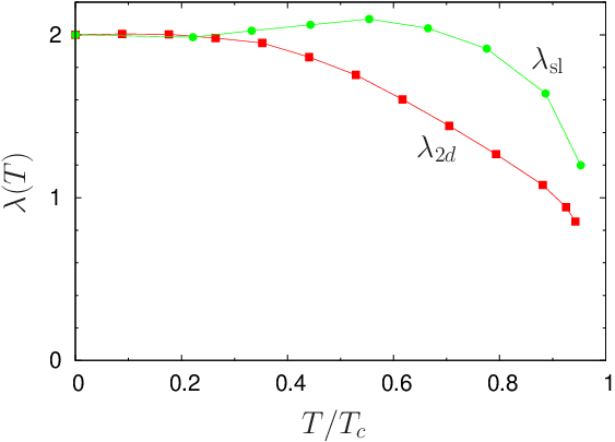
When the dynamics are affected by thermal noise, the behavior of depends on the dimensionality, as can be seen in Fig. 7. Although , within our numerical precision, monotonically decreases as the temperature increases towards [33, 42], this is not the case in . Since the system presents a large number of metastable states at [16, 17, 18], a small amount of noise may increase the wall velocity. Indeed, we find that has a maximum at intermediate temperatures. Nevertheless, although the temperature increases the roughness of the surface, the sliced disk still collapses more isotropically than the one, the fluctuations away from the circular shape being smaller. As the temperature approaches the critical value, tends to decrease to zero in both cases. It is, however, very hard to conclude about the exact -dependence in this range by tracking the evolution of a single initial volume. Some of the sources of difficulties are the fragmentation and merging processes that occur because of the thermal fluctuations. Analogously, for the case, isolated domains in the slice may belong to the same three-dimensional cluster.
III.2.2 Single toroidal domain
In the continuous description of coarsening the areas evolve independently of each other. Lattice effects do not affect this result at sufficiently large scales. However, although the dynamic mechanism in slices of a system is still curvature driven, the evolution of the areas on the slice may no longer be independent when, for instance, two different areas on a slice do belong to the same three dimensional domain.
A simple initial configuration that illustrates the importance of the third dimension and the new mechanism that may arise on the slice is a toroidal structure. In Fig. 8 we show the time evolution of an initial toroidal domain observed on a plane that contains its axis of revolution, that is, the initial state has two circular domains whose radii are the minor radius of the ring torus. The separation between their centers is twice the major radius . In the two cases shown in the figure, the minor radius is the same, , but the major radius is different: in (a) and in (b). The simulation is performed at . In both cases the whole toroid shrinks, and this can be seen as an effective attraction between the disks as they move towards each other. However, in the second case, the two initial disks change shape and, after some time, they merge and form an elongated domain in the plane. In the first case, the two disks do not merge on the observed timescale. Thus, differently from the pure case where such mechanism is absent, this merging process decreases the number of domains, increases the average area and thus slows down the rate at which the average area decreases.

Whether or not the results for , shown in this section for the evolution of a single domain, transpose to the coarsening problem, will be analyzed below. Moreover, to what extent the above merging mechanism has an important role in this case is an open problem.
III.3 Coarsening slices
When the initial state, instead of being prepared as a single sphere immersed in a sea of opposite spins, is taken from the equilibrium distribution at a given temperature above or at the critical point, much larger systems must be used in order to improve the statistics. Nonetheless, in severe restrictions on the total size of the system are imposed. We here consider systems with linear size up to and finite size effects may still be important.
In , the Ising model can be quenched to and yet evolve for a certain time before approaching either the ground state or a stripe state [15, 43], time that in many cases is enough to study coarsening phenomena [11, 12]. In , however, the dynamics get easily stuck in a sort of sponge state [16, 44, 17, 18]. To avoid this halting of the configuration evolution, after the system is equilibrated either at or , the quench is performed to a finite working temperature, , well below .
III.3.1
We start the analysis by checking that dynamic scaling applies to correlation functions measured on the slices in the usual way. In Fig. 9 we display the equal-time correlation between spins at a distance on the slice, , as a function of rescaled distance , for several times given in the key. The scaling is very satisfactory. In the inset we show the evaluation of the growing length scale using the criterium ; the straight line is the growth law of curvature driven dynamics with non-conserved order parameter. Notice that although they could be taken into account, we neglect the corrections to scaling linked to the time-scale discussed in Ref. [31] as they are not necessary for our purposes here.


At , the slices of the system are uncorrelated and any plane is statistically equivalent to a pure system. Since both species of spins have, on average, the same density, no domain percolates along the slices (on the square lattice, [24]) and the distributions of areas and perimeters do not behave critically at [11, 12] (see the corresponding curve in the inset of Fig. 10). However, once quenched to a subcritical temperature, the critical state of the site percolation is approached after a time that scales with the system size as . The exponent is 0.5 on the square lattice [31] but we have not analyzed the scaling of for the slices of the system, what would constitute a project on its own. Nonetheless, since the phenomenology of both and slices are similar (the area distribution soon develops a power law tail after the quench, as can be seen for and 4 in the inset of Fig. 10), we expect that will behave accordingly. In the whole volume, on the other hand, since the random site percolation threshold for the cubic lattice is , there are percolating clusters of both species of spins at . After the subcritical quench, the slices become correlated and the question we want to ask is to what extent the geometric properties, measured on a slice, resemble those of a system.


As can be seen in both Figs. 10 and 11, the exponent of the power-law tail increases with time. Its asymptotic value, for geometric domains (Fig. 10), is consistent with the critical percolation value, [24], although determining it precisely is a very hard task, as already discussed in Sec. II for the equilibrium data. For hull enclosed areas, Fig. 11, on the other hand, the convergence to the asymptotic exponent (2) is fast. The distributions for geometric domains contain all clusters, even those percolating, and present an overshoot region that does not change position as the system evolves (and thus moves to the left when we rescale the areas by time, as shown in the main panel). For the hull enclosed areas there is no peak associated to the percolating domains (that are excluded by definition), but at later times the system develops a maximum anyway. The curves in these figures (inset) present, in the course of time, two other regimes. They all display a plateau, that crosses over to the power-law tail, and a first, very rapid decay at very small areas. The former is the actual curvature driven regime. The latter are static and due to equilibrium temperature fluctuations. In Fig. 10 (inset) the black solid lines represent the analytic law, Eq. (14), with and . The constant takes the value used in Ref. [12] for the case. The factor in the numerator is associated to the high temperature initial condition. The parameter is very close in value to the one measured for the collapsing volume of a single sphere, see Sec. III.2, evaluated at the working temperature . Notice that even though the measurements are done on a slice, the relevant coefficient is the one obtained for the whole volume of the sphere. Analogously, in Fig. 11 (inset) the lines are Eq. (13) with the same coefficient and , again closely following the results [11]. Upon rescaling the areas by time, as required by dynamic scale invariance, a rather good collapse of all curves onto a universal curve is found, see Figs. 10 and 11 (main panels). As time increases, the power law tail of the distributions is less visible (for these small system sizes).
Areas and perimeters are also correlated [12, 41]. As an example, we present the collapsed curves (rescaling the area by and the perimeter by ) in Fig. 12 for the hull-enclosed areas and the corresponding perimeters (for geometric domains, the perimeter would also include the internal perimeters). Small domains are compact and round, thus . Large domains are reminiscent of the large domains created soon after the quench, when the power law developed, and one expects that area and perimeter are related as in critical percolation, [45]. Numerically, we find an exponent close to 1.2, compatible with the system value [12, 41], and with the results in Ref. [25] for the equilibrium clusters. In summary, within the numerical precision of our simulation, the dynamical behavior on a slice of a system is essentially equivalent to an actual system when the initial state is prepared at . The surprise is that instead of using the value of obtained from the measurements on a slice of the sphere, , the time evolving distribution of geometric domains uses related to the whole volume of the sphere, that is a half of the previous one, see Eq. (18).
III.3.2

As in the case, we start the analysis by checking that dynamic scaling applies to correlation functions measured on the slices also in the case in which the quench is performed from . We show in Fig. 13 the equal-time correlation between spins at a distance on the slice, , as a function of rescaled distance , for several times given in the key. Once again, the scaling is good. Notice also that the decay of the correlation keeps memory of the power-law present at the equilibrium state at , . Since the correlation is isotropic, measuring on a slice or in the whole volume would give the same behavior, thus, in the power-law exponent, and (the value for the Ising model). We present in the inset the growing length scale extracted from and the straight line .

When prepared in an equilibrium state at the critical temperature , several geometric distributions of the system present power law behavior since, in this case, the thermodynamical and the percolation transition coincide. Although this is no longer the case in in which the percolation critical temperature associated with geometric domains is smaller than the thermodynamical one, a slice presents critical behavior at and, as a consequence, one should find power-law behavior for several size distributions.
We saw in Sec. II that these distributions present strong finite size effects and, in particular, the exponents are smaller than expected. For example, the known exponent for the distribution of geometric domain areas in the critical IM is but this value is only approached asymptotically, for very large system sizes. For smaller rescaled sizes, the apparent exponent is even smaller than 2 what would bring normalization issues. These effects are even stronger in a sliced system, for which the data not even allow a clear extrapolation of the exponent. Besides differing in the behavior of the exponent, the coefficient of the power law distribution for a slice seems to have twice the value of the corresponding distribution. It is thus interesting to see how these differences occurring at evolve after the system is quenched to a temperature lower than the critical one.

After the quench, there seems to be a very fast crossover to a distribution without the extra factor 2 in the coefficient, see Fig. 14 (inset). This is observed in the behavior of the distribution for small areas, as it approaches a constant value that does not depend on the exponent, only on the coefficient and the measuring time. Indeed, the curves in Fig. 14 (inset) are well fitted using Eq. (14) without the factor 2 in the coefficient. However, for large areas, the tail of the distribution is not well described, as one would expect, by Eq. (14) and the exponent measured at , . We must notice, however, that the slices are small, thus the range of possible areas is rather limited. As time increases, the almost flat part of the distribution gets wider and the power law regime is hardly observed. In addition, the system suffers from finite size effects, even more severe than those for the case as discussed in the previous section, and the observed does not even extrapolate to the right value. Nevertheless, we still observe the correct scaling as shown in Fig. 14 (main panel). A similar behavior, but with an exponent slightly smaller, is shown in Fig. 15 for hull enclosed areas.
Areas and perimeters present, again, a two regimes relation. Small domains are round and . This first regime can be observed in the small part of Fig. 16, in which we related the size of a hull with the area that it encloses. Larger domains, on the other hand, still encode some information on its original shape and deviate from the circular format. Indeed, roughly above , the exponent decreases to 1.3. This value is compatible with previous estimates [25], yet well below the critical exponent [28], . Again the origin for such discrepancy may be the strong finite size effects previously discussed.

IV Conclusions
We addressed the differences between the clusters of a slice of a IM and the ones of an actual system, both in equilibrium and while coarsening.
We recalled that the clusters on slices of the IM are critical in equilibrium at (contrary to the structures). We found that the distribution of finite clusters, , has a larger weight on the slices than on the truly model, while a second very large (though still finite) cluster is mostly absent in the former while present in the latter. We showed that although working with rather large system sizes the measured exponents are still far from their asymptotic values when working on the slices.
Next we moved to the analysis of the geometric clusters and hull-enclosed areas that develop after instantaneous quenches from equilibrium at the infinite and the critical temperature. We found striking differences between the case with long range correlations in the initial state () and the case in which these do not exist (). In the absence of correlations, neighboring layers are independent, and even though strong correlations are built after a sudden subcritical quench, the subsequent behavior does not essentially differ (within our numerical precision) from the one found in the strictly case. On the other hand, for critical initial states, distant slices are correlated initially and such effect introduces differences between properties of the slices and the actual system. These differences already exist in the initial state, as explained in the previous paragraph. The extra weight on the finite size areas (a factor 2) seems to be washed out very rapidly after the quench and the small rescaled areas on the slices soon become very similar (identical within our numerical accuracy) to the ones of the system. Instead, the distribution and geometric properties of the large objects are much harder to characterize numerically on the slices as they are affected by strong finite size effects. Although we find that the data satisfy dynamic scaling we cannot draw precise conclusions about the exponent characterizing the tail of the distribution or the area-perimeter law as these are hard to determine numerically with good precision.
Work is in progress to extend these results to the IM with order parameter conserving dynamics and to the Potts model.
Acknowledgements.
JJA acknowledges the warm hospitality of the LPTHE (UPMC) in Paris during his stay where part of this work was done. JJA is partially supported by the INCT-Sistemas Complexos and the Brazilian agencies CNPq, CAPES and FAPERGS. LFC is a member of Institut Universitaire de France.References
- [1] A. J. Bray, Adv. Phys. 43, 357 (1994).
- [2] A. Onuki, Phase transition dynamics (Cambridge University Press, 2004).
- [3] S. Puri and V. Wadhawan, eds., Kinetics of phase transitions (Taylor and Francis Group, 2009).
- [4] W. R. White and P. Wiltzius, Phys. Rev. Lett. 75, 3012 (1995).
- [5] H. Jinnai, Y. Nishikawa, T. Koga, and T. Hashimoto, Macromolecules 28, 4782 (1995).
- [6] H. Jinnai, T. Koga, Y. Nishikawa, T. Hashimoto, and S. Hyde, Phys. Rev. Lett. 78, 2248 (1997).
- [7] H. Jinnai, Y. Nishikawa, and T. Hashimoto, Phys. Rev. E 59, R2554 (1999).
- [8] D. Bouttes, E. Gouillart, E. Boller, D. Dalmas, and D. Vandembroucq, Phys. Rev. Lett. 112, 245701 (2014).
- [9] J. Lambert, R. Mokso, I. Cantat, P. Cloetens, J. A. Glazier, F. Graner, and R. Delannay, Phys. Rev. Lett. 104, 248304 (2010).
- [10] I. Manke, N. Kardjilov, R. Schäfer, A. Hilger, M. Strobl, M. Dawson, C. Grünzweig, G. Behr, M. Hentschel, C. David, et al., Nat. Comm. 1, 125 (2010).
- [11] J. J. Arenzon, A. J. Bray, L. F. Cugliandolo, and A. Sicilia, Phys. Rev. Lett. 98, 145701 (2007).
- [12] A. Sicilia, J. J. Arenzon, A. J. Bray, and L. F. Cugliandolo, Phys. Rev. E 76, 061116 (2007).
- [13] M. Fialkowski, A. Aksimentiev, and R. Holyst, Phys. Rev. Lett. 86, 240 (2001).
- [14] M. Fialkowski and R. Holyst, Phys. Rev. E 66, 046121 (2002).
- [15] V. Spirin, P. L. Krapivsky, and S. Redner, Phys. Rev. E 63, 036118 (2001).
- [16] V. Spirin, P. Krapivsky, and S. Redner, Phys. Rev. E 65, 016119 (2002).
- [17] J. Olejarz, P. L. Krapivsky, and S. Redner, Phys. Rev. E 83, 051104 (2011a).
- [18] J. Olejarz, P. L. Krapivsky, and S. Redner, Phys. Rev. E 83, 030104 (2011b).
- [19] M. Newman and G. Barkema, Monte Carlo methods in statistical physics (Oxford University Press, New York, USA, 1999).
- [20] K. Binder, Ann. Phys. 98, 390 (1976).
- [21] A. Coniglio, C. R. Nappi, F. Peruggi, and L. Russo, J. Phys. A: Math. Gen. 10, 205 (1977).
- [22] H. Müller-Krumbhaar, Phys. Lett. A 50, 27 (1974).
- [23] A. L. Talapov and H. W. J. Blöte, J. Phys. A 29, 5727 (1996).
- [24] D. Stauffer and A. Aharony, Introduction To Percolation Theory (Taylor and Francis (London), 1994).
- [25] V. S. Dotsenko, M. Picco, P. Windey, G. Harris, E. Martinec, and E. Marinari, Nuc. Phys. B 448, 577 (1995).
- [26] A. A. Saberi and H. Dashti-Naserabadi, EPL 92, 67005 (2010).
- [27] J. L. Cambier and M. Nauenberg, Phys. Rev. B 34, 8071 (1986).
- [28] C. Vanderzande and A. L. Stella, J. Phys. A: Math. Gen. 22, L445 (1989).
- [29] A. L. Stella and C. Vanderzande, Phys. Rev. Lett. 62, 1067 (1989).
- [30] J. Cardy and R. M. Ziff, J. Stat. Phys. 110, 1 (2003).
- [31] T. Blanchard, F. Corberi, L. F. Cugliandolo, and M. Picco, EPL 106, 66001 (2014).
- [32] S. M. Allen and J. W. Cahn, Acta Metall. 27, 1085 (1979).
- [33] S. A. Safran, P. S. Sahni, and G. S. Grest, Phys. Rev. B 28, 2693 (1983).
- [34] K. A. Fichthorn and W. H. Weinberg, Phys. Rev. B 46, 13702 (1992).
- [35] M.-D. Lacasse, M. Grant, and J. Viñals, Phys. Rev. B 48, 3661 (1993).
- [36] D. Kandel and E. Domany, J. Stat. Phys. 58, 685 (1990).
- [37] L. Chayes, R. H. Schonmann, and G. Swindle, J. Stat. Phys. 79, 821 (1995).
- [38] P. Caputo, F. Martinelli, F. Simenhaus, and F. L. Toninelli, Comm. Pure and Applied Math. 64, 778 (2011).
- [39] H. Lacoin, Comm. Math. Phys. 318, 291 (2013).
- [40] M. P. O. Loureiro, J. J. Arenzon, L. F. Cugliandolo, and A. Sicilia, Phys. Rev. E 81, 021129 (2010).
- [41] M. P. O. Loureiro, J. J. Arenzon, and L. F. Cugliandolo, Phys. Rev. E 85, 021135 (2012).
- [42] M. Grant and J. D. Gunton, Phys. Rev. B 28, 5496 (1983).
- [43] T. Blanchard and M. Picco, Phys. Rev. E 88, 032131 (2013).
- [44] F. Corberi, E. Lippiello, and M. Zannetti, Phys. Rev. E 78, 011109 (2008).
- [45] H. Saleur and B. Duplantier, Phys. Rev. Lett. 58, 2325 (1987).