A discrete parametrized surface theory in ${\mathbb{R}}^{3}$

Tim Hoffmann ^†^†thanks: This research was supported by the DFG-Collaborative Research Center, TRR 109, “Discretization in Geometry and Dynamics.” Andrew O. Sageman-Furnas Max Wardetzky ^†^†thanks: This research was partially supported by the DFG-Collaborative Research Center, TRR 109, “Discretization in Geometry and Dynamics.”

Abstract

We propose a discrete surface theory in ${\mathbb{R}}^{3}$ that unites the most prevalent versions of discrete special parametrizations. This theory encapsulates a large class of discrete surfaces given by a Lax representation and, in particular, the one-parameter associated families of constant curvature surfaces. The theory is not restricted to integrable geometries, but extends to a general surface theory.

AMS 2010 subject classification: primary 53A05; secondary 52C99

1 Introduction

A quad net is a map from a strongly regular polytopal cell decomposition of a regular surface with all faces being quadrilaterals into ${\mathbb{R}}^{3}$ with nonvanishing straight edges. Notice, in particular, that nonplanar faces are admissible. In discrete differential geometry quad nets are understood as discretizations of parametrized surfaces [10, 11, 14]. In this agenda many classes of special surfaces have been discretized using algebro-geometric approaches for integrable geometry—originally using discrete analogues of soliton theory techniques (e.g., discrete Lax pairs and finite-gap integration [7]) to construct nets, but more recently using the notion of 3D consistency (reviewed in [11]).¹¹ 1 As in the smooth setting, these approaches have been successfully applied to space forms (see, e.g., [21, 3, 17, 16]). As an example consider the case of K-surfaces (i.e., surfaces of constant negative Gauß curvature). The integrability equations of classical surface theory are equivalent to the famous sine-Gordon equation [1, 19]. In an integrable discretization the sine-Gordon equation becomes a finite difference equation for which integrability is encoded by a certain closing condition around a 3D cube. Both in the smooth and discrete setting, integrability is bound to specific choices of parameterizations, such as asymptotic line parametrizations for K-surfaces. In this way different classes of surfaces, such as minimal surfaces or surfaces of constant mean curvature, lead to different PDEs and give rise to different parameterizations. In the discrete case, this is reflected by developments that treat different special surfaces by disparate approaches. These integrable discretizations maintain characteristic properties of their smooth counterparts (e.g., the transformation theory of Darboux, Bäcklund, Bianchi, etc.) and sometimes give rise to satisfying self-contained theories [13] within the special classes that they consider. What has been lacking, however, is a unified discrete theory that lifts the restriction to special surface parametrizations. Indeed, different from the case of classical smooth surface theory, existing literature does not provide a general discrete theory for quad nets.

We propose a theory that encompasses the most prevalent versions of existing discrete special parametrizations (reviewed in [9]), such as discrete conjugate nets [38], discrete (circular) curvature line nets [31, 18, 6], discrete isothermic nets [8, 12], and discrete asymptotic line nets [37, 42]. Our approach provides a curvature theory that, in particular, yields appropriate curvatures for previously defined discrete minimal [8], discrete constant mean curvature (cmc) [33, 9, 23], discrete constant negative Gauß curvature [37, 42, 7, 24, 34], and discrete developable surfaces [28]. This theory not only retrieves the curvature definitions given in [39, 15] in the case of planar faces but extends to the general setting of nonplanar quads. Moreover, for the first time, it provides a way to understand the one-parameter associated families of discrete surfaces of constant curvature, both in terms of discrete curvature and discrete conformality.

The fundamental property of our approach is the following edge-constraint that couples discrete surface points and normals: the average normal along an edge is perpendicular to that edge. This condition arises from a Steiner-type (i.e., offset and mixed area) perspective on curvature and, while surprisingly elementary, has profound consequences for the theory. By introducing a Gauß map for general nonplanar quad nets, our theory builds on basic construction principles of the classical smooth setting.

The paper is organized as follows: after the definition of edge-constraint nets (Section 2) we introduce their curvatures, naturally extending the work of Schief [39] and Bobenko, Pottmann, and Wallner [15]. These curvatures are then shown to be consistent with first, second, and third fundamental forms for edge-constraint nets. We describe the classical discrete integrable surfaces of constant curvature (circular minimal, circular cmc, and asymptotic and circular K-nets) and show that they are indeed edge-constraint nets of constant curvature (Section 3). Even more, we show that they possess associated families that are also edge-constraint nets exhibiting constant curvature. In particular, the proof for cmc nets shows a rather unexpected connection between their 3D compatibility cube and the general Bianchi permutability cube for discrete curves [25, 41]. The section closes with a discussion of discrete developable nets. We then provide a short treatment on how discrete conformality is represented in our theory (Section 4), showing that the members of the associated family of minimal nets are conformally equivalent. We conclude (Section 5) by showing that a rather general class of nets generated by a Sym–Bobenko formula is in fact a subset of edge-constraint nets.

2 Edge-constraint nets

2.1 Setup

A natural discrete analogue of a parametrized surface patch is a map from ${\mathbb{Z}}^{2}\to{\mathbb{R}}^{3}$ corresponding to a single chart. To consider discrete atlases we relax the combinatorial restrictions and think more generally of maps from quadrilateral graphs. We will use the words quadrilateral and quad interchangeably.

Definition 1 (Quadrilateral net).

A quad graph $\mathbb{G}$ is a strongly regular polytopal cell decomposition of a regular surface with all faces being quadrilaterals. A map $f:\mathbb{G}\to{\mathbb{R}}^{3}$ is called a (quad) net.

Figure 1: Shift notation used to describe the points of a quad net

f

, even with irregular combinatorics.

Remark (Shift notation).

As seen in Figure 1, we will use shift notation [11] to describe the points of a quad net: when the underlying quad graph has the combinatorics of ${\mathbb{Z}}^{2}$ , we denote a point by $f=f_{k,l}$ for some $k,l\in{\mathbb{Z}}$ and define the shift operators $f_{1}:=f_{k+1,l}$ and $f_{2}:=f_{k,l+1}$ . The point diagonal to $f$ is given by a shift in each direction, $f_{12}:=f_{k+1,l+1}$ . In what follows we do not restrict ourselves to the combinatorics of ${\mathbb{Z}}^{2}$ , but will continue to use shift notation, as there is no ambiguity when the discussion is restricted to a point $f$ ; oriented edge $f_{i}-f$ with $i=1,2$ ; or quad $(f,f_{1},f_{12},f_{2})$ .

Immersed parametrized surfaces in the smooth setting can be thought of either as a smooth family of points or as the envelope of a family of tangent planes. One defines a contact element at a point $p\in{\mathbb{R}}^{2}$ of a parametrized surface $f:D\subset{\mathbb{R}}^{2}\to{\mathbb{R}}^{3}$ as the pair $(f(p),P(p))$ , consisting of a point $f(p)$ and the oriented tangent plane $P(p)$ passing through it. $P(p)$ is completely determined by its unit normal $n(p)$ when anchored at $f(p)$ ; considering $n(p)$ at the origin defines the Gauss map $n:D\subset{\mathbb{R}}^{2}\to{\mathbb{S}^{2}}$ . Using this perspective we consider parametrized surfaces as the pair of maps $(f,n)$ , an immersion together with its Gauß map.

Analogously we consider discrete parametrized surfaces not as a single quad net, but as a pair of nets that are weakly coupled, mimicking the relationship between an immersion and its Gauß map in the smooth setting. This pair will be known as an edge-constraint net and is our main object of study.

Definition 2 (Edge-constraint net).

Let $\mathbb{G}$ be a quad graph. We call a pair of quadrilateral nets $(f,n):\mathbb{G}\to{\mathbb{R}}^{3}\times{\mathbb{S}^{2}}$ a contact element net. A contact element net is called an edge-constraint net if it satisfies the following:

Edge-constraint: For each pair of points of $f$ connected by an edge, the average of the normals at those points is perpendicular to the edge, i.e., for $i=1,2$ we have $f_{i}-f\perp\frac{1}{2}(n_{i}+n)$ .

We further assume that $f$ contains no vanishing edges, i.e., that $f_{i}-f$ is always nonzero.

The maps $f:\mathbb{G}\to{\mathbb{R}}^{3}$ and $n:\mathbb{G}\to{\mathbb{S}^{2}}$ are called the (discrete) immersion and Gauß map, respectively.

Remark.

As edge-constraint nets are in fact a pair of nets, unless we state explicitly that we are referring only to the immersion $f$ or the Gauß map $n$ , the combinatorial language of vertex, edge, face (or quad) will refer to the combinatorics of the underlying quad graph $\mathbb{G}$ .

The edge-constraint discretizes a coupling between the Gauß map and immersion; in the smooth setting it is generic in the following sense.

Lemma 3.

Let $f:{\mathbb{R}}^{2}\to{\mathbb{R}}^{3}$ parametrize a smooth surface patch with Gauß map $n:{\mathbb{R}}^{2}\to{\mathbb{S}^{2}}$ . For every point $p\in{\mathbb{R}}^{2}$ and unit vector $v\in{\mathbb{R}}^{2}$ , let the images of the line $p+tv$ where $t\in{\mathbb{R}}$ be given (with a slight abuse of notation) by $f(t):=f(p+tv)$ and $n(t):=n(p+tv)$ , respectively. Then the central and one-sided difference approximations to the edge-constraint along $f(t)$ are satisfied up to second order, i.e.,

	$\displaystyle(f(\epsilon)-f(-\epsilon))\cdot(n(\epsilon)+n(-\epsilon))$	$\displaystyle=$	$\displaystyle 0+O(\epsilon^{3})~\mathrm{and}~$
	$\displaystyle(f(\epsilon)-f(0))\cdot(n(\epsilon)+n(0))$	$\displaystyle=$	$\displaystyle 0+O(\epsilon^{3}).$

Proof.

Note that $f^{\prime}(t)\cdot n(t)=0$ by construction, so in particular $f^{\prime\prime}(t)\cdot n(t)+f^{\prime}(x)\cdot n^{\prime}(t)=0$ . The statement then follows by Taylor expanding $f(t)$ and $n(t)$ around $t=0$ with small parameter $\epsilon>0$ . ∎

The simplest class of edge-constraint nets are those given by quadrilateral nets in spheres.

Lemma 4.

Let $f:\mathbb{G}\to r{\mathbb{S}^{2}}$ be a quad net in the sphere of radius $r>0$ . Then $f$ together with the Gauß map $n=f/r$ is an edge-constraint net.

Edge-constraint nets naturally exhibit offset nets by adding multiples of the Gauß map to the original immersion while keeping the Gauß map fixed. This observation is the foundation of their curvature theory.

Lemma 5 (Offset nets).

For any $t\in{\mathbb{R}}$ and contact element net $(f,n):\mathbb{G}\to{\mathbb{R}}^{3}\times{\mathbb{S}^{2}}$ , the contact element net $(f+t\,n,n)$ , where linear combinations are taken on vertices, is an edge-constraint net if and only if $(f,n)$ is an edge-constraint net.

2.2 Curvatures from Offsets

Let $f:{\mathbb{R}}^{2}\to{\mathbb{R}}^{3}$ be a smooth parametrized surface with Gauß map $n:{\mathbb{R}}^{2}\to{\mathbb{R}}^{3}$ . For each $t\in{\mathbb{R}}$ and $(x,y)\in{\mathbb{R}}^{2}$ we define the offset surface by $f^{t}(x,y):=f(x,y)+t\,n(x,y)$ . We only consider smooth parametrizations $f$ which give rise to smooth offsets $f^{t}$ for small enough $|t|$ . It is easily seen that $n$ is also the Gauß map for the offset surface $f^{t}$ , thus the construction of offset nets seen in Lemma 5. For all $(x,y)\in{\mathbb{R}}^{2}$ , the area element at $f^{t}(x,y)$ can be expressed in terms of the area element, mean and Gauß curvatures at $f(x,y)$ . This relationship is known as the Steiner formula and is best understood through the mixed area form.

Definition 6 (Mixed area form).

Let $g,h:{\mathbb{R}}^{2}\to{\mathbb{R}}^{3}$ parametrize two smooth surfaces that share a Gauß map $N:{\mathbb{R}}^{2}\to{\mathbb{S}^{2}}$ . For every $(x,y)\in{\mathbb{R}}^{2}$ , we define the mixed area form in the tangent plane $P\perp N(x,y)$ by

A(g,h):=\frac{1}{2}(\det(g_{x},h_{y},N)+\det(h_{x},g_{y},N)),

(1)

where subscripts denote partial derivatives. When $g=h$ , the mixed area form reduces to the area element of $g$ .

Remark.

To define the mixed area form we switched notation to a capital $N,$ as opposed to little $n$ , for the Gauß map. While in the smooth setting these two objects coincide, the discrete Gauß map for an edge-constraint net (also denoted by $n$ ) lives on vertices, whereas we will define the mixed area form for an edge-constraint net on faces. We will define a new unit vector per face, which we call the projection direction (denoted by $N$ ), that defines the tangent plane $P$ where this mixed area form lives.

We can now state the Steiner formula and consequently define the mean and Gauß curvature functions on a smooth parametrized surface. The same definitions will carry over to edge-constraint nets.

Theorem 7 (Steiner formula).

Let $f:{\mathbb{R}}^{2}\to{\mathbb{R}}^{3}$ be a smooth surface parametrization with Gauß map $n:{\mathbb{R}}^{2}\to{\mathbb{R}}^{3}$ and offset surface $f^{t}:{\mathbb{R}}^{2}\to{\mathbb{R}}^{3}$ . Then for each $(x,y)\in{\mathbb{R}}^{2}$ the following relationship holds

	$\displaystyle A(f^{t},f^{t})$	$\displaystyle=$	$\displaystyle A(f,f)+2tA(f,n)+t^{2}A(n,n),$		(2)
		$\displaystyle=$	$\displaystyle(1+2t\mathcal{H}+t^{2}\mathcal{K})A(f,f),$		(2)

defining

\mathcal{H}:=\frac{A(f,n)}{A(f,f)}~\mathrm{and}~\mathcal{K}:=\frac{A(n,n)}{A(f,f)},

(3)

as the mean and Gauß curvature functions, respectively.

Figure 2: The partial derivatives,

n_{x}

and

n_{y}

, of a (possibly non-planar) quadrilateral from the Gauß map

n

of an edge-constraint net as defined by the midpoint connectors. A projection direction,

N\perp n_{x},n_{y}

is also shown, determining the face tangent plane

P

where the mixed area form is defined.

Definition 8.

Consider a single quadrilateral from an edge-constraint net $(f,n)$ . We define the partial derivatives as the midpoint connectors of the (possibly non-planar) quadrilaterals for each of $f$ and $n$ , e.g., for the Gauß map, as shown in Figure 2, we have

n_{x}:=\frac{1}{2}(n_{12}+n_{1})-\frac{1}{2}(n_{2}+n),~n_{y}:=\frac{1}{2}(n_{12}+n_{2})-\frac{1}{2}(n_{1}+n),

(4)

and likewise for $f$ . Then the set of admissible projection directions is defined as

U:=\{N\in{\mathbb{S}^{2}}|~N\perp\mathop{\mathrm{span}}{\{n_{x},n_{y}\}}\}.

(5)

Generically, the projection direction is unique (up to sign) and we choose

N:=\frac{n_{x}\times n_{y}}{\|n_{x}\times n_{y}\|}.

(6)

In the (quad) tangent plane $P\perp N$ we define the (discrete) mixed area form via Equation (1), yielding a Steiner formula (Equation (2)).

Remark (Degenerate Gauß maps).

The set of admissible projection directions also generates a consistent curvature theory in the degenerate situation where the partial derivatives of the Gauß map are not linearly independent. Degenerate Gauß maps naturally arise in the theory of developable surfaces, so we defer this discussion to the theory of developable edge-constraint nets in Section 3.4.

Definition 9 (Edge-constraint curvatures).

Using the Steiner formula (Equation (2)) we define mean and Gauß curvatures for edge-constraint nets via Equation (3).

Remark (Degenerate immersions).

Clearly the curvatures are only well defined when the immersion has non-vanishing area $A(f,f)\neq 0$ . Every statement we make about curvatures will assume the immersion quad has non-vanishing area.

Remark (Sign of projection direction).

The sign of the projection direction in the generic setting does not correspond to a change in local orientation. The mixed area form will obviously change sign, but the mean and Gauß curvatures are invariant to this choice. However, flipping the Gauß map ( $n\to-n$ ) does change the sign of the mean curvature, as expected.

Remark (Choice of partial derivatives).

The choice to define the partial derivatives as the midpoint connectors is to guide intuition. In fact, one has the freedom to choose any linear combination of the midpoint connectors to be the partial derivatives, as long as the same combination is chosen for both the immersion and the Gauß map. This corresponds to the freedom to locally reparametrize in the smooth setting. The mean and Gauß curvatures and forthcoming definitions of principal curvatures and curvature line fields are all invariant to this choice. As expected, the mixed area forms and fundamental forms will change as these are not invariant to a local reparametrization in the smooth setting either.

In the smooth setting one can also derive the mean and Gauß curvatures at a point via the fundamental forms and shape operator living in the tangent plane to that point. The shape operator is a real self-adjoint bilinear form whose eigenvalues and eigenvectors are the principal curvatures and curvature lines, respectively. From Definition 8 we can discretize the fundamental forms and shape operator in the plane perpendicular to the projection direction of each face of an edge-constraint net.

Definition 10 (Fundamental forms).

Consider a single quad from an edge-constraint net $(f,n)$ . Let $\pi$ be the projection into the quad tangent plane P. Set $\hat{f}_{x}:=\pi(f_{x})=f_{x}-(f_{x}\cdot N)N$ and similarly for $\hat{f}_{y}$ .²² 2 Since $N\perp n_{x},n_{y}$ by Definition 8, $\hat{n}_{x}=n_{x}$ and $\hat{n}_{y}=n_{y}$ . We define the fundamental forms and shape operator by:

	$\displaystyle\mathrm{I}$	$\displaystyle:=\left(\begin{array}[]{cc}\hat{f}_{x}\cdot\hat{f}_{x}&\hat{f}_{x}\cdot\hat{f}_{y}\\ \hat{f}_{y}\cdot\hat{f}_{x}&\hat{f}_{y}\cdot\hat{f}_{y}\end{array}\right),~~\mathrm{II}$	$\displaystyle:=\left(\begin{array}[]{cc}\hat{f}_{x}\cdot n_{x}&\hat{f}_{x}\cdot n_{y}\\ \hat{f}_{y}\cdot n_{x}&\hat{f}_{y}\cdot n_{y}\end{array}\right),$
	$\displaystyle\mathrm{III}$	$\displaystyle:=\left(\begin{array}[]{cc}n_{x}\cdot n_{x}&n_{x}\cdot n_{y}\\ n_{y}\cdot n_{x}&n_{y}\cdot n_{y}\end{array}\right),~~\mathcal{S}$	$\displaystyle:=~\mathrm{I}^{-1}\mathrm{II}.$

The eigenvalues $(k_{1},k_{2})$ and eigenvectors of the shape operator $S$ are the principal curvatures and curvature line fields of the quadrilateral.

The existence of principal curvatures and curvature line fields follows from the symmetry of the second fundamental form:

Lemma 11.

Consider a single quad from an edge-constraint net $(f,n)$ , then the second fundamental form is symmetric.

Proof.

In the above notation we want to show $\hat{f}_{x}\cdot n_{y}-n_{x}\cdot\hat{f}_{y}=0$ . As $N\perp n_{x},n_{y}$ this quantity is the same when unprojected, i.e.,

\hat{f}_{x}\cdot n_{y}-n_{x}\cdot\hat{f}_{y}=f_{x}\cdot n_{y}-n_{x}\cdot f_{y}.

(15)

Expanding out $f_{x}\cdot n_{y}-n_{x}\cdot f_{y}$ one finds it is a constant multiple of the sum of the edge-constraint conditions once around the quadrilateral, which vanishes as it vanishes on each edge by assumption. ∎

The mean and Gauß curvatures per quadrilateral defined via the Steiner formula are equal to the ones derived from the eigenvalues of the shape operator.

Lemma 12 (Curvature and fundamental form relationships).

The following relations hold true in the smooth and discrete case:
1. $\mathcal{K}=k_{1}\,k_{2}=\det\mathrm{II}/\det\mathrm{I}$ ,
2. $\mathcal{H}=\frac{1}{2}\left(k_{1}+k_{2}\right)$ ,
3. $\mathrm{III}-2\mathcal{H}\,\mathrm{II}+\mathcal{K}\,\mathrm{I}=0$ , and
4. $A(f,f)^{2}=\det\mathrm{I}$ .

Example (Spherical edge-constraint nets).

Let $(f,f/r)$ be an edge-constraint net in the sphere of radius $r>0$ as determined by Lemma 4. Then every quadrilateral has the expected Gauß ( $\mathcal{K}=\frac{1}{r^{2}}$ ) and mean curvature ( $\mathcal{H}=\frac{1}{r}$ ).

Example (Curvature line fields).

Figure 3 shows the curvature line fields of an ellipsoid in the smooth and discrete setting.

Refer to caption — Figure 3: Left: Curvature lines of a smooth ellipsoid. Middle: Curvature line field of an ellipsoid edge-constraint net. Right: Overlay of smooth and discrete curvature line fields.

3 Constant Curvature Nets

Edge-constraint nets and their curvature theory provide a unifying geometric framework through which to understand previously defined notions of discrete surfaces of constant curvature in special parametrizations. Due to their governing integrable structure, these surfaces naturally arise in one parameter associated families that in the smooth setting fix the respective curvature, but change the type of parametrization. Previous notions of discrete curvature exist for each particular type of special parametrization, but have been difficult to reconcile with the corresponding (differently parametrized) associated families.

In what follows we rectify these discrepancies by showing that the algebraically constructed discrete isothermic minimal surfaces [8]; discrete isothermic constant mean curvature surfaces [8]; discrete asymptotic line constant negative Gauß curvature surfaces [7]; and discrete curvature line constant negative Gauß curvature surfaces [27], together with each of their respective associated families are in fact edge-constraint nets with their respective curvatures constant. To close we introduce a theory of developable edge-constraint nets, a non-integrable example.

3.1 Discrete minimal surfaces

We start with the general definition.

Definition 13 (Minimal edge-constraint net).

An edge-constraint net $(f,n)$ is called minimal if every quad has vanishing mean curvature ( $\mathcal{H}=0$ ), i.e., the mixed area $A(f,n)$ vanishes.

In the smooth setting, minimal surfaces are often parametrized by isothermic (curvature line and conformal) coordinates arising naturally form their construction from holomorphic Weierstrass data: Stereographically project a holomorphic function $g:\mathbb{C}\to\mathbb{C}$ onto the Riemann sphere to get a conformal map $n:\mathbb{C}\to{\mathbb{S}^{2}}$ . Now, think of $n$ as the Gauß map to a surface and construct the Christoffel dual isothermic surface $f:\mathbb{C}\to{\mathbb{R}}^{3}$ by integrating

f_{x}(x,y)=\frac{n_{x}(x,y)}{\|n_{x}(x,y)\|^{2}}\mathrm{~~and~~}f_{y}(x,y)=-\frac{n_{y}(x,y)}{\|n_{y}(x,y)\|^{2}}.

(16)

The resulting $f$ is an isothermic parametrization of a minimal surface in ${\mathbb{R}}^{3}$ with Gauß map given by the conformal map $n$ . This process of generating a minimal surface is called the Weierstrass representation.

Bobenko and Pinkall defined discrete minimal surfaces as a special case of discrete isothermic surfaces and showed they exhibit a discrete Weierstrass representation [8]. These nets indeed have vanishing mean curvature in a curvature theory for nets with planar faces (that in the case of contact element nets is contained in the present theory) [39, 15].

In complete analogy to the smooth case, one can extend this representation into an associated family. This corresponds to locally rotating the frame, therefore changing the type of parametrization away from being curvature line (while staying conformal in the smooth setting). While this is an algebraic way to define the discrete nets of the associated family there has been no notion through which one can understand their minimality. The goal of this section is to rectify this by showing that every member of the associated family is an edge-constraint net and that its mean curvature vanishes on every quad.

Formulating the discrete Weierstrass representation requires discrete analogues of curvature line parametrizations, Christoffel duals, and isothermic parametrizations. We briefly introduce these notions, but emphasize that each of these discrete objects is interesting in its own right (see the book by Bobenko and Suris [11]).

Definition 14 (Circular net).

A contact element net $(f,n)$ is called a circular net or discrete curvature line net if:
1. every quad of the immersion $f$ is circular, its vertices lie on a circle; and
2. the Gauß map along each edge is found by reflection through the immersion edge perpendicular bisector plane, i.e., for $i=1,2$ we have

n=n_{i}-2\frac{n_{i}\cdot(f_{i}-f)}{\|f_{i}-f\|^{2}}(f_{i}-f).

(17)

Lemma 15.

Let $(f,n)$ be a circular net, then it is an edge-constraint net.

Proof.

Equation (17) gives: $f_{i}-f\parallel n_{i}-n\perp n_{i}+n$ . ∎

Note that the symmetry imposed by the second property implies that the Gauß map and all offset nets $(f+tn,n)$ are also circular nets, with corresponding quads lying in parallel planes.

Definition 16 (Isothermic net).

Let $(f,n)$ be a circular net. Then $(f,n)$ is a discrete isothermic net if there exists a second circular net $(f^{*},n)$ with the same Gauß map such that $A(f,f^{*})=0$ . The net $(f^{*},n)$ is unique (up to scaling and translation) and called the discrete Christoffel dual net of $(f,n)$ .

We now state a few important properties of discrete isothermic nets that we will need [12].

Lemma 17.

Let $(f,n)$ be a discrete isothermic net with Christoffel dual $(f^{*},n)$ . Then the following hold:
1. There exists real values $\beta$ per edge that coincide for opposite edges on each quad and the cross-ratio of every quad factorizes, i.e.,

\frac{(f_{1}-f)(f_{12}-f_{2})}{(f_{12}-f_{1})(f_{2}-f)}=\frac{\beta_{1}}{\beta_{2}},

(18)

with $\beta_{1}=\beta_{f_{1}-f}$ and $\beta_{2}=\beta_{f_{2}-f}$ associated to shifts in the first and second lattice directions, respectivly.
2. Corresponding edges of $f$ and $f^{*}$ are parallel and satisfy:

f^{*}_{i}-f^{*}=\beta_{i}\frac{f_{i}-f}{\|f_{i}-f\|^{2}}~\mathrm{for}~i=1,2,

(19)

while non-corresponding diagonals are parallel and satisfy:

f^{*}_{12}-f^{*}=(\beta_{2}-\beta_{1})\frac{f_{2}-f_{1}}{\|f_{2}-f_{1}\|^{2}}~\mathrm{and}~f^{*}_{2}-f^{*}_{1}=(\beta_{2}-\beta_{1})\frac{f_{12}-f}{\|f_{12}-f\|^{2}}.

(20)

For the rest of this section we restrict the discussion to the special case of discrete isothermic nets whose immersion quads have cross-ratio minus one, in particular, we will assume that $\beta_{1}=1$ and $\beta_{2}=-1$ for every quad. The reason for doing this is that if we think of the cross-ratio as a discrete analog of $f_{x}^{2}/f_{y}^{2}$ , then cross-ratio minus one corresponds to $f_{x}^{2}=-f_{y}^{2}$ , the defining property of conformal maps; the more general notion of factorizing cross-ratio allows for reparametrizations of the parameter lines.

It is essential to emphasize that the restriction to cross-ratio minus one solely serves the purpose of simplifying the algebra. Every result that follows also holds with the more general definition, with the pre-factors $\beta_{1}$ and $\beta_{2}$ cropping up in the expected places.

The notion of a discrete holomorphic function just restricts the notion of discrete isothermicity to the plane.

Definition 18.

Fix a quad graph $\mathbb{G}$ . The complex function $g:\mathbb{G}\to\mathbb{C}$ is called a discrete holomorphic function if every quad has cross-ratio minus one.

We can now define the discrete Weierstrass representation by following the same procedure as in the smooth case.

Definition 19 (Weierstrass representation of discrete isothermic minimal nets).

Let $g:{\mathbb{Z}}^{2}\to\mathbb{C}$ be a discrete holomorphic function and consider the discrete isothermic net $(f,n)$ where:
1. the Gauß map $n$ is given by the stereographic projection of the holomorphic data $g$ , i.e.,

	$\displaystyle n$	$\displaystyle:=$	$\displaystyle\frac{1}{1+\|g\|^{2}}(g+\bar{g},\frac{1}{i}(g-\bar{g}),\|g\|^{2}-1),\mathrm{~so~in~particular~}$		(21)
	$\displaystyle n_{i}$	$\displaystyle:=$	$\displaystyle\frac{1}{1+\|g_{i}\|^{2}}(g_{i}+\bar{g}_{i},\frac{1}{i}(g_{i}-\bar{g}_{i}),\|g_{i}\|^{2}-1)\mathrm{~for~}i=1,2;$

2. and $f$ is given (up to translations) as the discrete isothermic dual immersion of $n$ , i.e., for a shift in either direction

	$\displaystyle f_{1}-f:=\frac{n_{1}-n}{\\|n_{1}-n\\|^{2}}=\Re\left(\frac{1}{2(g_{1}-g)}(1-g_{1}g,i(1+g_{1}g),g_{1}+g)\right)\mathrm{and}$
	$\displaystyle f_{2}-f:=-\frac{n_{2}-n}{\\|n_{2}-n\\|^{2}}=-\Re\left(\frac{1}{2(g_{2}-g)}(1-g_{2}g,i(1+g_{2}g),g_{2}+g)\right).$		(22)

We call the arising net a discrete isothermic minimal net.

Lemma 20.

Let $(f,n)$ be a discrete isothermic minimal net. Then it is a minimal edge-constraint net.

Proof.

Discrete isothermic nets are circular nets, so they are edge-constraint nets and by construction $(f,n)$ is the Christoffel dual of $(n,n)$ , so $A(f,n)=0$ . ∎

In the smooth setting the Weierstrass representation provides a way to compute the Gauß curvature explicitly and for isothermic surfaces is given by $\mathcal{K}=\frac{-4|g^{\prime}|^{4}}{(1+|g|^{2})^{4}}$ , see [32]. This has a discrete analogue:

Lemma 21.

Let $(f,n)$ be a discrete isothermic minimal net arising from a discrete holomorphic function $g:{\mathbb{Z}}^{2}\to\mathbb{C}$ . Then the Gauß curvature of a quad is given in terms of $g$ by:

\mathcal{K}=\frac{-4(|g_{12}-g||g_{2}-g_{1}|)^{2}}{(1+|g|^{2})(1+|g_{1}|^{2})(1+|g_{12}|^{2})(1+|g_{2}|^{2})}.

(23)

Proof.

Again we use the diagonals as the discrete partial derivatives. By Equation (20) we have $A(f,f)=-\frac{4}{\|n_{x}\|^{2}\|n_{y}\|^{2}}A(n,n)$ . Recall that the chordal distance between the stereographic projection of two points $w$ and $z$ in $\mathbb{C}$ is

\frac{2}{\sqrt{(1+|z|^{2})(1+|w|^{2})}}|z-w|.

(24)

Applying this to $\|n_{x}\|^{2}$ and $\|n_{y}\|^{2}$ explicitly recovers the result. ∎

The discrete Weierstrass representation naturally gives rise to an associated family. We think of the discrete Weierstrass representation in terms of the corresponding discrete complex Weierstrass vectors

\omega_{i}=\frac{1}{2(g_{i}-g)}(1-g_{i}g,i(1+g_{i}g),g_{i}+g)

(25)

for each lattice direction $i=1,2$ so that the immersion edges can be concisely written: $f_{1}-f=\Re\omega_{1}$ and $f_{2}-f=-\Re\omega_{2}$ .

Definition 22 (Associated family of discrete isothermic minimal net).

Let $g:{\mathbb{Z}}^{2}\to\mathbb{C}$ be a discrete holomorphic function, $n:{\mathbb{Z}}^{2}\to{\mathbb{S}^{2}}$ be the stereographic projection of $g$ , $\omega_{i}$ be the discrete complex Weierstrass vectors of $g$ , and $\lambda=e^{i\alpha}$ for $\alpha\in[0,2\pi]$ . Then the family of contact element nets $(f^{\alpha},n)$ given by:

f_{1}^{\alpha}-f^{\alpha}:=\Re(\lambda\omega_{1})\mathrm{~and~}f_{2}^{\alpha}-f^{\alpha}:=-\Re(\lambda\omega_{2})

(26)

is called the associated family of the discrete isothermic minimal net $(f^{0},n)$ and $\lambda$ is called the spectral parameter.

Lemma 23.

Let $(f^{0},n)$ be a discrete isothermic minimal net. Any member $(f^{\alpha},n)$ of its associated family is an edge-constraint net as well.

Proof.

By formally extending the dot product to complex 3-vectors³³ 3 By the complex formal dot product we mean $(z_{1},z_{2},z_{3})\cdot(w_{1},w_{2},w_{3}):=\sum_{i=1}^{3}z_{i}w_{i}$ ; there is no conjugation in the second component. and noting that the Gauß map $n\in{\mathbb{R}}^{3}$ is real valued we have for $i=1,2$ that $\Re(\lambda\omega_{i})\cdot n=\Re(\lambda\omega_{i}\cdot n)$ and $\Re(\lambda\omega_{i})\cdot n_{i}=\Re(\lambda\omega_{i}\cdot n_{i})$ . We easily compute $\Re(\lambda\omega_{1}\cdot n)=-\Re(\frac{\lambda}{2})$ and $\Re(\lambda\omega_{1}\cdot n_{1})=\Re(\frac{\lambda}{2})$ . Similarly, $\Re(\lambda\omega_{2}\cdot n)=\Re(\frac{\lambda}{2})$ and $\Re(\lambda\omega_{2}\cdot n_{2})=-\Re(\frac{\lambda}{2})$ . So $(f^{\alpha}_{i}-f^{\alpha})\cdot n=-(f^{\alpha}_{i}-f\alpha)\cdot n_{i}$ . ∎

The previous lemma provides us with a way to interpret the rotation generated by the multiplication of $\lambda$ directly in ${\mathbb{R}}^{3}$ :

Figure 5: The geometry of an edge in the associated family (Equation (27)) along with its original immersion edge (that is parallel to its Gauß map edge); the circle is the circumcircle of an adjacent Gauß map quadrilateral whose properties are needed to understand the geometry of immersion quads in the associated family (Lemma 25).

Lemma 24.

Let $(f^{\alpha},n)$ be the associated family of a discrete isothermic minimal net $(f^{0},n)$ . Then for each $\alpha\in[0,2\pi]$ and $i=1,2$ we have:

f^{\alpha}_{i}-f^{\alpha}=(-1)^{(i-1)}\|f^{0}_{i}-f^{0}\|^{2}(\cos\alpha(n_{i}-n)-\sin\alpha(n_{i}\times n)).

(27)

In other words $f^{\alpha}_{i}-f^{\alpha}$ is given by $f^{0}_{i}-f^{0}$ rotated in the plane perpendicular to $(n_{i}+n)$ by angle $\alpha$ , as shown in Figure 5.

Proof.

We show the result for the first lattice direction $i=1$ , the other lattice direction follows similarly.

For every $\alpha\in[0,2\pi]$ the immersion edge $f^{\alpha}_{1}-f^{\alpha}$ is perpendicular to $(n_{1}+n)/2$ , so it is a linear combination of $(n_{1}-n)$ and $(n_{1}\times n)$ . Furthermore, in terms of the complex discrete Weierstass vector, this immersion edge is the linear combination $\Re(\lambda\omega_{1})=\cos\alpha\Re\omega_{1}-\sin\alpha\Im\omega_{1}$ . Since $(f^{0},n)$ and $(n,n)$ are dual discrete isothermic nets we immediately have $\Re\omega_{1}=\|f^{0}_{1}-f^{0}\|^{2}(n_{1}-n)$ , so we only have to show $\Im\omega_{1}=\|f^{0}_{1}-f^{0}\|^{2}(n_{1}\times n)$ .

A simple computation yields that the formal complex 3-vector dot product $\omega_{1}\cdot\omega_{1}$ is real and equal to $1/4$ . In particular, this implies that the real dot product $\Re\omega_{1}\cdot\Im\omega_{1}=0$ and that $\|\Im\omega_{1}\|^{2}=\|\Re\omega_{1}\|^{2}-1/4$ . Hence $\Im\omega_{1}$ is parallel to $n_{1}\times n$ (since it is perpendicular to both $(n_{1}-n)$ and $(n_{1}+n)$ ). Now, since the Gauß map vectors are unit length we have $\|n_{1}\times n\|^{2}=\|\frac{n_{1}+n}{2}\|^{2}\|n_{1}-n\|^{2}$ , which we use to conclude

\|\Im\omega_{1}\|^{2}=\frac{1}{\|n_{1}-n\|^{2}}-1/4=\frac{\|n_{1}+n\|^{2}}{4\|n_{1}-n\|^{2}}=(\|f^{0}_{1}-f^{0}\|^{2}\|n_{1}\times n\|)^{2}.

(28)

∎

Figure 6: A non-planar quad (blue) from the associated family of a discrete isothermic minimal net and its projection, which is a rotated and scaled version of the original circular quad (black). Note that the Gauß map is constant.

This more geometric construction of the associated family highlights the following important relationship (shown in Figure 6), which will lead to vanishing mean curvature.

Lemma 25 (Quad geometry of the associated family).

Every immersion quad of a member of the associated family $(f^{\alpha},n)$ when projected into its corresponding Gauß map plane is a scaled and rotated version of its corresponding circular immersion quad of $(f^{0},n)$ .

Proof.

We show that an immersion edge of $(f^{\alpha},n)$ when projected into one of its neighboring Gauß map planes is a scaled and rotated version of its corresponding immersion edge of $(f^{0},n)$ ; the setup is given in Figure 5. In particular, the scaling factor and rotation angle are independent of the lattice direction, so the result extends to the quads, proving the lemma.

What follows is identical for both lattice directions, so we work with the first one. The Gauß map quad is circular so the projection direction $N$ anchored at the origin passes through its circumcenter (at height $d$ ) and is normal to its plane; let $\pi$ be the projection into this plane. Furthermore, $N\perp(n_{1}-n)$ so from Equation (27) we see that

\pi(f^{\alpha}_{1}-f^{\alpha})=(\|f^{0}_{1}-f^{0}\|)^{2}(\cos\alpha(n_{1}-n)-\sin\alpha\cos\phi(n_{1}\times n)),

(29)

where $\phi$ is the angle between $f^{\alpha}_{1}-f^{\alpha}$ and the Gauß map plane. Observe that the angle between $N$ and $\frac{n_{1}+n}{2}$ is also $\phi$ , so we can calculate:

$\displaystyle\\|\pi(f^{\alpha}_{1}-f^{\alpha})\\|^{2}$	$\displaystyle=$	$\displaystyle(\\|f^{0}_{1}-f^{0}\\|)^{4}(\cos^{2}\alpha(l)^{2}+\sin^{2}\alpha\cos^{2}\phi\\|n_{1}\times n\\|^{2})$	(30)
	$\displaystyle=$	$\displaystyle(\\|f^{0}_{1}-f^{0}\\|)^{2}(\cos^{2}\alpha+\sin^{2}\alpha\cos^{2}\phi\\|\frac{n_{1}+n}{2}\\|^{2}).$
	$\displaystyle=$	$\displaystyle(\\|f^{0}_{1}-f^{0}\\|)^{2}(\cos^{2}\alpha+\sin^{2}\alpha~d^{2}).$

Therefore, the projected edge length is the original edge length scaled by a factor $\varsigma$ that is independent of the lattice direction and rotated by angle $\theta$ , i.e.,

\varsigma=\sqrt{\cos^{2}\alpha+\sin^{2}\alpha~d^{2}}~~\mathrm{and}~~\cos\theta=\frac{\cos\alpha}{\sqrt{\cos^{2}\alpha+\sin^{2}\alpha~d^{2}}}.

(31)

∎

We can now prove the main result of this section.

Theorem 26 (Minimality of the associated family).

All contact element nets $(f^{\alpha},n)_{\alpha\in[0,2\pi]}$ in the associated family of a discrete isothermic minimal net $(f^{0},n)$ are minimal edge-constraint nets.

Proof.

Choose an arbitrary $\alpha\in[0,2\pi]$ . Consider a single quad of $(f^{\alpha},n)$ with projection direction $N$ , projection map $\pi$ and partial derivatives given by the diagonals. By Lemma 25 there exist a rotation by angle $\theta$ in the plane perpendicular to $N$ and a scaling factor $\varsigma$ (both depending on $\alpha$ ) that bring the original immersion quad of $f^{0}$ into the projected associated family quad of $f^{\alpha}$ . Noticing that $\cos\alpha$ equals zero or one exactly when $\cos\theta$ is also zero or one, respectively, we write:

	$\displaystyle\pi(f^{\alpha}_{x})$	$\displaystyle=$	$\displaystyle\varsigma\\|f^{0}_{x}\\|(\cos\theta\frac{f^{0}_{x}}{\\|f^{0}_{x}\\|}+\sin\theta\frac{f^{0}_{y}}{\\|f^{0}_{y}\\|})~\mathrm{and}$
	$\displaystyle\pi(f^{\alpha}_{y})$	$\displaystyle=$	$\displaystyle\varsigma\\|f^{0}_{y}\\|(-\sin\theta\frac{f^{0}_{x}}{\\|f^{0}_{x}\\|}+\cos\theta\frac{f^{0}_{y}}{\\|f^{0}_{y}\\|}).$		(32)

The original net $(f^{0},n)$ is discrete isothermic so Equation (20) implies that: $\frac{f^{0}_{x}}{\|f^{0}_{x}\|}=-\frac{n_{y}}{\|n_{y}\|}$ and $\frac{f^{0}_{y}}{\|f^{0}_{y}\|}=-\frac{n_{x}}{\|n_{x}\|}$ ; and that $\|f^{0}_{x}\|\|n_{y}\|=\|n_{x}\|\|f^{0}_{y}\|=2$ . Therefore, we compute twice the mixed area and see that it vanishes.

$\displaystyle 2A(f^{\alpha},n)$	$\displaystyle=$	$\displaystyle\det(\pi(f^{\alpha}_{x}),n_{y},N)+\det(n_{x},\pi(f^{\alpha}_{y}),N)$	(33)
	$\displaystyle=$	$\displaystyle-2\varsigma(\det(\sin\theta\frac{n_{x}}{\\|n_{x}\\|},\frac{n_{y}}{\\|n_{y}\\|},N)+\det(\frac{n_{x}}{\\|n_{x}\\|},-\sin\theta\frac{n_{y}}{\\|n_{y}\\|},N))$
	$\displaystyle=$	$\displaystyle 0.$

∎

In contrast to the smooth case, the Gauß curvature does not stay constant in the discrete associated family, but it changes in a controlled way:

Theorem 27 (Gauß curvature of the associated family).

Let $(f^{\alpha},n)$ be contact element net in the associated family of a discrete isothermic minimal net $(f^{0},n)$ and let $\mathcal{K}^{\alpha}$ and $\mathcal{K}^{0}$ be their respective Gauß curvatures. Then

\mathcal{K}^{\alpha}=\frac{\mathcal{K}^{0}}{\varsigma^{2}},

(34)

where $\varsigma^{2}=\cos^{2}\alpha+\sin^{2}\alpha~d^{2}$ is the square of the scaling factor as above and $d$ is the distance to the circumcenter of the corresponding Gauß map quad.

Note that $\varsigma$ will approach one in the continuum limit.

Proof.

By Lemma 25 we have $A(f^{\alpha},f^{\alpha})=\varsigma^{2}A(f^{0},f^{0})$ and $A(n,n)$ is constant throughout the family. ∎

As in the smooth case we can define the conjugate discrete isothermic minimal net of $(f^{0},n)$ as $(f^{\frac{\pi}{2}},n)$ . The members of the associated family are linear combinations of the discrete isothermic net and its conjugate net, since $(f^{\frac{\pi}{2}},n)$ arises as the imaginary part of the complex Weierstrass vectors. The conjugate net is known to be in asymptotic line parametrization. Discrete analogues of such parametrizations are known as A-nets and were originally introduced by Sauer [37] and Wunderlich [42] to investigate surfaces of constant negative Gauß curvature (as we will do in Section 3.3).

Definition 28 (Discrete asymptotic net).

An edge-constraint net is an A-net if its immersion has planar vertex stars (i.e., if all immersion edges meeting at a vertex lie in a common plane) and the Gauß map is given by choosing unit normals to these planes.

This definition corresponds to the fact that the osculating planes of asymptotic lines are the tangential planes of the surface.

Lemma 29.

Every A-net is an edge-constraint net.

Proof.

This follows directly from the definition. ∎

We close by showing that conjugate discrete isothermic minimal nets are indeed A-nets.

Lemma 30.

The conjugate net $(f^{\frac{\pi}{2}},n)$ of a discrete isothermic minimal net $(f^{0},n)$ is an A-net.

Proof.

From equation (27) the edges of the conjugate net satisfy:

f^{\frac{\pi}{2}}_{1}-f^{\frac{\pi}{2}}=-\|f^{0}_{1}-f^{0}\|(n_{1}\times n)~\mathrm{and}~f^{\frac{\pi}{2}}_{2}-f^{\frac{\pi}{2}}=\|f^{0}_{2}-f^{0}\|(n_{2}\times n).

(35)

In particular, this means that all edges emanating from a generic vertex of $f^{\frac{\pi}{2}}$ are perpendicular to the corresponding Gauss map $n$ , which is the definition of an A-net. ∎

3.2 Discrete constant mean curvature surfaces

We start with a general definition.

Definition 31 (Constant mean curvature edge-constraint net).

An edge-constraint net $(f,n)$ is said to have constant mean curvature if every quad of the net has the same non-vanishing mean curvature $\mathcal{H}\in{\mathbb{R}}^{*}$ .

Like their simpler minimal cousins, smooth surfaces of constant mean curvature are often described in isothermic parametrizations. In such coordinates the Gauß-Codazzi equation is given in terms of the conformal metric parameter $u$ (defined by $ds^{2}=e^{u}(dx^{2}+dy^{2})$ ), and reduces to the integrable elliptic sinh-Gordon equation,

u_{xy}=\sinh(u).

(36)

Techniques of soliton theory have been immensely successful in explicitly constructing and classifying constant mean curvature surfaces (e.g., tori [35, 4]) in the classical setting of Euclidean three-space and other space forms. The integrability condition of a suitably gauged frame can be identified with the Lax representation of the integrable equation [40, 5] which harnesses methods from soliton theory for geometry and allows for structure preserving discretizations [11]. Moreover, one can then explicitly describe the immersed surfaces in terms of the so-called Sym–Bobenko formula, which by construction simultaneously generates the associated family.

Using this method Bobenko & Pinkall [9] defined discrete constant mean curvature surfaces as a subclass of discrete isothermic surfaces, just as they did for discrete minimal surfaces. For smooth constant mean curvature surfaces the DPW method [20] is a Weierstrass type method that allows the construction of all cmc surfaces from holomorphic / meromorphic data. A discrete version of this method giving rise to the same frame description as Bobenko & Pinkall can be found in [23].

As with the minimal case, these discrete isothermic surfaces arising from the frame description have previously been shown to have constant mean curvature [15], but once again, the naturally arising associated family leaves the realm of the special isothermic parametrization (to more general conformal parametrizations in the smooth setting). Thus there has been no notion of discrete mean curvature through which this family could be geometrically understood. Again, we rectify this by showing that the original discrete isothermic net and its entire algebraically generated associated family are in fact constant mean curvature edge-constraint nets.

Since the curvature theory of edge-constraint nets satisfies the Steiner formula (Equation (2)), the linear Weingarten relationship and its corollary come for free by calculating the curvatures of an offset surface.

Lemma 32 (Linear Weingarten relationship).

Let $(f,n)$ be an edge-constraint net. Then for any $t\in{\mathbb{R}}$ the edge-constraint net given by the offset $f^{t}=(f+tn,n)$ has curvatures

\mathcal{K}_{f^{t}}=\frac{\mathcal{K}}{1+2\mathcal{H}t+\mathcal{K}t^{2}}~\mathrm{and}~\mathcal{H}_{f^{t}}=\frac{\mathcal{H}+\mathcal{K}t}{1+2\mathcal{H}t+\mathcal{K}t^{2}},

(37)

where $\mathcal{K},\mathcal{H}$ are the Gauß and mean curvatures of the original surface $(f,n)$ . If $(f,n)$ has constant mean curvature, then there exist $\alpha,\beta\in{\mathbb{R}}$ only depending on $t,\mathcal{H}$ such that

\alpha\mathcal{K}_{f^{t}}+\beta\mathcal{H}_{f^{t}}=1.

(38)

In other words, for each offset net, $\alpha,\beta$ are constant on all quads of the net.

Proof.

Choose $\alpha=-t(\frac{1}{\mathcal{H}}+t)$ and $\beta=\frac{1}{\mathcal{H}}+2t$ . ∎

An important corollary is that constant mean curvature edge-constraint nets come in pairs, just like their smooth counterparts (see Figure 7).

Corollary 33.

Let $(f,n)$ be a constant mean curvature edge-constraint net with mean curvature $\mathcal{H}=-\frac{1}{h}$ , for some $h\in{\mathbb{R}}^{+}$ . Then the offset net $(f^{*},n):=(f+hn,n)$ is also a constant mean curvature edge-constraint net with mean curvature $\mathcal{H}^{*}=-\mathcal{H}$ and the middle edge-constraint net $(\hat{f},n):=(f+\frac{h}{2}n,n)$ has constant positive Gauß curvature $4\mathcal{H}^{2}$ .

Remark.

If $(f,n)$ is a discrete isothermic net of constant mean curvature $\mathcal{H}=-\frac{1}{h}$ then the offset net $(f+hn,n)$ is in fact the discrete Christoffel dual isothermic net (Definition 16).

For simplicity for the rest of our discussion we rescale to $\mathcal{H}=-1$ .

Lemma 34.

Let $(f,n)$ be an edge-constraint net with unit offset $(f^{*},n):=(f+n,n)$ . Consider a single quad, then

A(f,f^{*})=0\iff\mathcal{H}=A(f,n)/A(f,f)=-1.

(39)

In other words, vanishing mixed area between a net and its unit offset for every quad is equivalent to both nets having constant mean curvature. The condition

A(f,f^{*})=\det(f_{12}-f,f_{2}^{*}-f_{1}^{*},N)+\det(f_{12}^{*}-f^{*},f_{2}-f_{1},N)=0

(40)

can be understood geometrically as the vanishing sum of the (projected) areas of the curves formed by $f,f_{1}^{*},f_{12},f_{2}^{*}$ and $f^{*},f_{1},f_{12}^{*},f_{2}$ which we denote $g$ and $g^{*}$ , respectively:

		$\displaystyle g=f,g_{1}=f_{1}^{},g_{12}=f_{12},~\mathrm{and}~g_{2}=f_{2}^{};$	$\displaystyle~\mathrm{and}$		(41)
		$\displaystyle g^{}=f^{},g_{1}^{}=f_{1},g_{12}^{}=f_{12}^{},~\mathrm{and}~g_{2}^{}=f_{2}.$			(41)

Therefore, to prove that an edge-constraint net has constant mean curvature we switch between the two combinatorial cubes $C_{f}$ and $C_{g}$ formed by $f,f^{*}$ and $g,g^{*}$ , respectively. They share the same vertex set but the edges of one are the diagonals of the other.

By showing that the algebraically generated associated family of discrete constant mean curvature nets of Bobenko and Pinkall [9] are constant mean curvature edge-constraint nets, we find that their $C_{g}$ cubes are built from skew parallelograms, yielding an unexpected connection to the 3D compatibility cube for discrete curves from the theory of integrable systems [25, 41]. We now briefly recapitulate the moving frame description of these nets.

We identify Euclidean three space ${\mathbb{R}}^{3}$ with the imaginary part of the quaternions $\mathbb{H}=\mathop{\mathrm{span}}{\{\mathbbm{1},\mathbbm{i},\mathbbm{j},\mathbbm{k}\}}$ , i.e., ${\mathbb{R}}^{3}\cong\mathop{\mathrm{span}}{\{\mathbbm{i},\mathbbm{j},\mathbbm{k}\}}\cong\mathop{\mathrm{span}}{\{-i\sigma_{1},-i\sigma_{2},-i\sigma_{3}\}}$ , where

\sigma_{1}=\left(\begin{array}[]{cc}0&1\\ 1&0\end{array}\right),~\sigma_{2}=\left(\begin{array}[]{cc}0&-i\\ i&0\end{array}\right),~\sigma_{3}=\left(\begin{array}[]{cc}1&0\\ 0&-1\end{array}\right),

(42)

are the 2x2 complex Pauli matrices generating the Lie algebra su(2). Using this representation one describes the surface via a moving frame $\Phi\in\Im\mathbb{H}$ which rotates the orthonormal frame of ${\mathbb{R}}^{3}$ into the surface tangent plane and normal vector. Specifically, conjugation by a quaternion corresponds to a rotation and the frame encodes the Gauß map directly by rotating $\mathbbm{k}$ , i.e., $n=-i\Phi^{-1}\sigma_{3}\Phi=\Phi^{-1}\mathbbm{k}\Phi$ . These frame descriptions are the natural language of integrable systems related to surface theory both smooth and discrete [5, 9, 11].

Figure 8: Shift notation for the frame description. The frame of a net

\Phi

lives on vertices, while the corresponding Lax matrices

U

and

V

live on edges; for both the frame and Lax matrices one can understand shifts in either lattice direction.

With the notation of Figure 8, we introduce the frame $\Phi$ of interest [9] by initially setting $\Phi$ equal to the identity and then defining the vertex shifts

\Phi_{1}:=U\Phi~\mathrm{and}~\Phi_{2}:=V\Phi,

(43)

where

U:=\left(\begin{array}[]{cc}a&-\lambda u-\frac{1}{\lambda u}\\ \frac{u}{\lambda}+\frac{\lambda}{u}&\bar{a}\end{array}\right)~\mathrm{and}~V:=\left(\begin{array}[]{cc}b&-i\lambda v+\frac{i}{\lambda v}\\ i\frac{\lambda}{v}-\frac{i}{\lambda}v&\bar{b}\end{array}\right)

(44)

are the Lax matrices with spectral parameter $\lambda=e^{i\alpha}$ for $\alpha\in[0,2\pi]$ , $a,b$ complex valued functions living on vertices (and $\bar{a},\bar{b}$ their complex conjugates), and $u,v$ positive real valued functions living on vertices. To guarantee that each quad closes, i.e., $\Phi_{12}=\Phi_{21}$ , the Lax matrices and their shifts $V_{1}$ and $U_{2}$ must satisfy the compatibility condition (with determinants splitting evenly):

V_{1}U=U_{2}V,~\mathrm{with}~\det(U)=\det(U_{2})~\mathrm{and}~\det(V)=\det(V_{1}).

(45)

For every value of the spectral parameter the net is then generated by taking the imaginary part⁴⁴ 4 Unlike in [9] we purposefully do not normalize the transport matrices $U$ and $V$ to have determinant 1. Thus $\Phi$ is not in $SU(2)$ , necessitating taking the imaginary part. of the Sym–Bobenko formula [9] (an example is shown in Figure 9),

$\displaystyle n$	$\displaystyle:=$	$\displaystyle\Phi^{-1}\mathbbm{k}\Phi$
$\displaystyle\mathbbm{f}$	$\displaystyle:=$	$\displaystyle\left(-\Phi^{-1}\frac{d}{d\alpha}\Phi\|_{\lambda=e^{i\alpha}}+\frac{1}{2}\Phi^{-1}\mathbbm{k}\Phi\right),$	(46)
$\displaystyle f$	$\displaystyle:=$	$\displaystyle\Im\mathbbm{f}.$

Definition 35 (Associated family).

Let $(f,n):=(f^{\alpha},n^{\alpha})$ be a net generated from the frame $\Phi$ (with spectral parameter $\lambda=e^{i\alpha}$ ) given by Equations (44), (45), and (46). We call $(f,n)$ a member of the associated family of a discrete isothermic constant mean curvature net.

Lemma 36.

Every member of the associated family of a discrete isothermic constant mean curvature net is an edge-constraint net. Furthermore, for $i=1,2$ the edge-constraint is expressed in the equations

n_{i}=-(\mathbbm{f}_{i}-\mathbbm{f})n(\mathbbm{f}_{i}-\mathbbm{f})^{-1}.

(47)

Proof.

We defer the proof to Section 5 where a general discussion of edge-constraint nets arising from Lax pairs is provided. ∎

In general, the edge-constraint can be understood along a shift in either lattice direction $i=1,2$ as first negating $n$ and then rotating it along the edge $f_{i}-f$ to find $n_{i}$ , which, when written quaternionically, gives rise to the following definition.

Definition 37 (Normal transport quaternions).

Consider a quad from an edge-constraint net $(f,n)$ . The quaternions given by $\phi:=\tau+(f_{1}-f),\tau\in{\mathbb{R}}$ and $\psi=\eta+(f_{2}-f),\eta\in{\mathbb{R}}$ such that

n_{1}=-\phi^{-1}n\phi~\mathrm{and}~n_{2}=-\psi^{-1}n\psi,

(48)

are called normal transport quaternions.⁵⁵ 5 Although inverses naturally arise on the right (Equation (47)) from the Sym–Bobenko formula, we prefer to define normal transports with inverses on the left; this simply corresponds to an opposite sign convention for the real part of the normal transport.

This perspective yields insight into the geometry of the cubes $C_{f}$ and $C_{g}$ for an arbitrary edge-constraint net.

Lemma 38 (Edge-constraint as a skew parallelogram).

Let $(f,n)$ be an edge-constraint net with offset net $(f^{*},n)=(f+n,n)$ . For each quad, consider the combinatorial cubes $C_{f}$ and $C_{g}$ formed by it and its offset (as given in Equation (41)). Then the four sides of $C_{f}$ and $C_{g}$ are skew trapezoids and skew parallelograms, respectively.

Moreover, we will see that if $(f,n)$ is a member of the associated family of a discrete isothermic constant mean curvature net then for every quad we have the following three facts, that together imply that $(f,n)$ has constant mean curvature: (i) the top and bottom of $C_{g}$ are also parallelograms; (ii) all six sides are parallelograms of the same ”folding parameter”, so $C_{g}$ forms an ”equally-folded parallelogram cube”; and (iii) every equally-folded parallelogram cube has vanishing (projected) mixed area between its top and bottom.

Let $g,g_{1},g_{12},g_{2}$ be a skew parallelogram built from the edge lengths $\ell_{1}$ and $\ell_{2}$ . It is straightforward to see that the dihedral angles $\delta_{1}$ and $\delta_{2}$ (measured between $0$ and $\frac{\pi}{2}$ ) along the diagonals of this skew parallelogram (understood as edges of the enclosing tetrahedron) satisfy $\frac{\sin\delta_{1}}{\ell_{1}}=\frac{\sin\delta_{2}}{\ell_{2}}$ .

Definition 39.

The folding parameter of a skew parallelogram with the above notation is defined as

\sigma:=\frac{\sin\delta_{1}}{\ell_{1}}=\frac{\sin\delta_{2}}{\ell_{2}}.

(49)

Lemma 40.

Every skew parallelogram can be written in terms of two edges $g_{1}-g$ and $g_{2}-g$ with lengths $\ell_{1}$ and $\ell_{2}$ , respectively, and a folding parameter $\sigma$ :

	$\displaystyle g_{12}-g_{2}=(\rho\mathbbm{1}+(g_{2}-g_{1}))(g_{1}-g)(\rho\mathbbm{1}+(g_{2}-g_{1}))^{-1},$
	$\displaystyle\mathrm{where}~\rho=\frac{1}{\sigma}\left(\sqrt{1-\sigma^{2}\ell_{1}^{2}}-\sqrt{1-\sigma^{2}\ell_{2}^{2}}\right).$		(50)

Proof.

The real part $\rho$ is the same as $\Re\nu$ in Equation 3.15 of [25], with $k=\tan\frac{\delta_{1}}{2}\cot\frac{\delta_{2}}{2}$ and $s=\ell_{1}$ . Using Jacobi Elliptic functions one can rewrite this expression to find the above equation. ∎

This construction can be extended to three edges and a fixed folding parameter, yielding the known combinatorial 3D compatibility cube of skew parallelograms [25, 41]:

Theorem 41 (Darboux transform for parallelograms).

Let $g$ be a skew parallelogram with edge lengths $\ell_{1},\ell_{2}$ and folding parameter $\sigma$ . For every initial vector $\tilde{n}\in{\mathbb{R}}^{3}$ there exists a unique skew parallelogram $g^{*}$ at constant distance $\|\tilde{n}\|$ from $g$ such that:
1. $g^{*}$ also has edge lengths $\ell_{1},\ell_{2}$ and folding parameter $\sigma$ ; and
2. every face of the combinatorial cube $C_{g}$ formed by $g$ and $g^{*}$ is a skew parallelogram of folding parameter $\sigma$ .
We call this object an equally-folded parallelogram cube.⁶⁶ 6 Instead of fixing the folding parameter $\sigma$ one can also hold the real part $\rho$ constant; this is also 3D compatible as shown in [36].

Proof.

Recall that $g$ itself can be generated from the two vectors $w_{1}:=g_{1}-g$ and $w_{2}:=g_{2}-g$ and the folding parameter $\sigma$ . Therefore, we can rephrase the theorem statement as: Given $w_{1},w_{2},\tilde{n}$ and the folding parameter $\sigma$ , show that completing the skew parallelogram twice in every direction forms a closed combinatorial cube. This is precisely the Bianchi Permutability Theorem for a single edge in the Darboux (Bäcklund) transformation of a discrete arc-length parametrized curve, a proof of which is given in [25]. ∎

We now come back to the viewpoint that one can switch between the combinatorial cubes $C_{g}$ and $C_{f}$ as introduced in Equation (41).

Theorem 42.

Consider an equally-folded parallelogram cube $C_{g}$ with bottom and top $g$ and $g^{*}$ , respectively. Let $h\in{\mathbb{R}}$ be the constant distance between $g$ and $g^{*}$ . Then the bottom and top quads of the corresponding cube $C_{f}$ with normals given by the vertical edges of $C_{f}$ are edge-constraint net quads with mean curvatures $-\frac{1}{h}$ and $\frac{1}{h}$ , respectively.

Proof.

Notice that $C_{g}$ can be constructed from three vectors and a folding parameter using the simplified equation for the real part of the rotation quaternions, Equation (50). Using the quaternionic description and $\hat{G}:=((g_{12}^{*}-g_{12})-(g^{*}-g))\times((g_{2}-g_{2}^{*})-(g_{1}-g_{1}^{*}))$ one finds that

\det(g_{12}^{*}-g^{*},g_{2}^{*}-g_{1}^{*},\hat{G})+\det(g_{12}-g,g_{2}-g_{1},\hat{G})=0.

(51)

Using that $N\parallel\hat{G}$ , this is equivalent to $A(f,f^{*})=A(f,f+hn)=0$ . Therefore, the edge-constraint quads $(f,n)$ and $(f+hn,n)$ indeed have mean curvatures - $\frac{1}{h}$ and $\frac{1}{h}$ . ∎

Remark.

The top and bottom faces in the previous theorem can be exchanged for any pair of opposite faces (i.e., front and back or left and right). It turns out that the direction of $\hat{G}$ defined in the previous proof is independent of this choice (possibly up to sign). In other words, the quad tangent planes arising from every pair of opposite faces coincide.

Theorem 43.

Let $(f,n)$ be a member of the associated family of a discrete isothermic constant mean curvature net (Definition 35) with spectral parameter $\lambda=e^{i\alpha}$ . Then $(f,n)$ is a constant mean curvature edge-constraint net.

Proof.

By Lemma 36 $(f,n)$ is an edge-constraint net. Consider the unit offset net $(f^{*},n)=(f+n,n)$ . For every quad we show that the corresponding combinatorial cube $C_{g}$ is an equally-folded parallelogram cube; the result then follows from Theorem 42.

We naturally extend the quaternionic description of $f=\Im\mathbbm{f}$ and $f^{*}=\Im(\mathbbm{f}+n)$ to $g:=\Im\mathbbm{g}$ and $g^{*}:=\Im\mathbbm{g}^{*}$ , e.g., $\mathbbm{g}_{1}^{*}-\mathbbm{g}=\mathbbm{f}_{1}-\mathbbm{f}$ . The non-unit edges of the parallelograms of the front and left sides of $C_{g}$ are found to have squared lengths:

		$\displaystyle\ell_{1}^{2}:=\\|g_{1}-g\\|^{2}=1-4(\frac{\cos(2\alpha)}{\det(U)}+\frac{\sin^{2}(2\alpha)}{\det(U)^{2}})$	$\displaystyle~\mathrm{and}$		(52)
		$\displaystyle\ell_{2}^{2}:=\\|g_{2}-g\\|^{2}=1+4(\frac{\cos(2\alpha)}{\det(V)}-\frac{\sin^{2}(2\alpha)}{\det(V)^{2}}).$			(52)

Recall that by assumption $\det(U)=\det(U_{2})$ and $\det(V)=\det(V_{1})$ , so the back and right sides of $C_{g}$ are also parallelograms with non-unit edge lengths $\ell_{1}$ and $\ell_{2}$ , respectively. Therefore, the top and bottom of $C_{g}$ are also parallelograms both built from the edge lengths $\ell_{1}$ and $\ell_{2}$ .

The transports (in the sense of Lemma 40) that yield the front, left, and top skew parallelograms of $C_{g}$ are:

$\displaystyle-n_{1}=(\mathbbm{g}_{1}^{}-\mathbbm{g})n(\mathbbm{g}_{1}^{}-\mathbbm{g})^{-1},$		(53)
$\displaystyle-n_{2}=(\mathbbm{g}_{2}^{}-\mathbbm{g})n(\mathbbm{g}_{2}^{}-\mathbbm{g})^{-1},$	$\displaystyle~\mathrm{and}$
$\displaystyle\mathbbm{g}_{12}-\mathbbm{g}_{2}=(\mathbbm{g}_{2}-\mathbbm{g}_{1})(\mathbbm{g}_{1}-\mathbbm{g})(\mathbbm{g}_{2}-\mathbbm{g}_{1})^{-1}.$

The real parts arising from the Sym–Bobenko formula for corresponding edges, e.g., $\Re(\mathbbm{f}_{1}-\mathbbm{f})=\frac{1}{2}\mathop{\mathrm{tr}}(U^{-1}\frac{\partial}{\partial\alpha}U)$ , can be computed directly using the derivative of the determinant:

\frac{\partial}{\partial\alpha}\det(U)=\det(U)\mathop{\mathrm{tr}}(U^{-1}\frac{\partial}{\partial\alpha}U).

(54)

Applying this formula to the ”double transport”, e.g. $V_{1}U$ , shows that the sum of the real parts of $\mathbbm{f}_{1}-\mathbbm{f}$ and $\mathbbm{f}_{12}-\mathbbm{f}_{1}$ is in fact the real part of the diagonal transport furnished by $\mathbbm{f}_{12}-\mathbbm{f}$ . We therefore find:

	$\displaystyle\Re(\mathbbm{g}_{1}^{*}-\mathbbm{g})=\frac{2\sin(2\alpha)}{\det(U)},$
	$\displaystyle\Re(\mathbbm{g}_{2}^{*}-\mathbbm{g})=-\frac{2\sin(2\alpha)}{\det(V)},~\mathrm{and}$		(55)
	$\displaystyle\Re(\mathbbm{g}_{2}-\mathbbm{g}_{1})=\Re(\mathbbm{g}_{2}-\mathbbm{g})-\Re(\mathbbm{g}_{1}-\mathbbm{g})=-\frac{(\det(U)+\det(V))\sin(2\alpha)}{\det(U)\det(V)}.$

Plugging the real parts from Equations (55) with the edge lengths from Equations (52) into the Equation (50) yields the folding parameter $\sigma=\sin(2\alpha)$ in every instance.

Therefore $C_{g}$ is an equally-folded parallelogram cube. ∎

3.3 Discrete constant negative Gauß curvature surfaces

We start with a general definition motivated by the smooth setting.

Definition 44 (Constant negative curvature edge-constraint nets).

An edge-constraint net $(f,n)$ is said to have constant negative (Gauß) curvature if every quad of the net has the same negative non-vanishing Gauß curvature $\mathcal{K}\in{\mathbb{R}}^{-}$ .

A surface parametrized by asymptotic lines has constant negative Gauß curvature if and only if the asymptotic lines form a Chebyshev net, i.e., the parameter lines are parallel transports of each other in the sense of Levi-Civita. Thus, the directional derivative along each parameter line depends only on a single variable, so its integral curve exhibits a constant speed parametrization (possibly a different constant for each parameter line); Chebyshev nets are made up of ”infinitesimal parallelograms” with side lengths $a,b\in{\mathbb{R}}^{+}$ . Furthermore, the Gauß map of the asymptotic lines also form a Chebyshev net on the sphere. In these coordinates, the Gauß-Codazzi equation reduces to the well known sine-Gordon equation in the angle between the asymptote lines $u(x,y)$ :

-\mathcal{K}ab\sin u(x,y)=u_{xy}(x,y).

(56)

This equation is invariant to the transformation $a\to\lambda a$ and $b\to\lambda^{-1}b$ for all $\lambda=e^{t}$ with $t\in{\mathbb{R}}$ ; varying $\lambda$ generates the associated family of a constant negative curvature asymptotic line parameterized surface, where the angles between the asymptotic lines are invariant.

From the above characterization Sauer [37, 38] defined the following discrete analogue.

Definition 45 (K-nets).

An edge-constraint net $(f,n):D\subset{\mathbb{Z}}^{2}\to{\mathbb{R}}^{3}\times{\mathbb{S}^{2}}$ is a K-net if it is an A-net and there exists two lengths $a,b>0$ such that every immersion quad is a skew parallelogram (Chebyshev quad) with edge lengths $a$ and $b$ . ⁷⁷ 7 For K-nets we restrict to regular combinatorics because having more than two asymptotic lines meet at a point is incompatible with having negative Gauß curvature.

Note that the Gauß map of a K-net is also built from Chebyshev quads.

The associated family for K-nets was defined geometrically by Wunderlich [42] using a transformation that, like in the smooth setting, preserves the interior angles of $f$ while scaling its edges. These geometric constructions agree with an algebraic description (similar to that introduced for constant mean curvature nets in the previous section) in terms of a discrete sine-Gordon equation and its Lax pair that is then integrated via a Sym–Bobenko formula to construct the net [7, 24]. However, due to the inherent non-planarity of the quads in these nets, understanding their curvatures has remained elusive. The goal of this section is to show (using the geometric constructions) that K-nets indeed have constant negative Gauß curvature as edge-constraint nets.

K-nets can be constructed (up to global rotation and scale) directly from Cauchy data for their Gauß map [34]. Explicitly, a fourth Gauß map point $n_{12}$ is determined by completing the skew parallelogram through three other points $n,n_{1},n_{2}\in{\mathbb{S}^{2}}$ : ⁸⁸ 8 In other words the Gauß map satisfies the discrete Moutard equation in ${\mathbb{S}^{2}}$ [30].

n_{12}:=\frac{n\cdot(n_{1}+n_{2})}{1+n_{1}\cdot n_{2}}(n_{1}+n_{2})-n.

(57)

The immersion $f$ is constructed from $n$ via

f_{1}-f:=n_{1}\times n~\mathrm{and}~f_{2}-f:=n\times n_{2}.

(58)

When $n_{i}\cdot n=\cos\Delta_{i}$ the edge lengths of $f$ are given by $\sin\Delta_{i}$ for $i=1,2$ . Moreover, applying Napier’s analogies to the spherical parallelogram formed by $n$ the two interior angles $\alpha,\beta\in(0,\pi)$ of a K-net immersion quad are related by $e^{i\alpha}=\frac{e^{i\beta}k-1}{e^{i\beta}-k}$ , where $k=\tan\frac{\Delta_{1}}{2}\tan\frac{\Delta_{2}}{2}$ [7].

The associated family can now be described by a family of pairs of Gauß map angles $(\Delta_{1}(\lambda),\Delta_{2}(\lambda))$ from which the K-nets are explicitly constructed.

Definition 46 (K-net associated family).

Consider a K-net $(f,n)$ with the above notation and let $\lambda=e^{t}$ for all $t\in{\mathbb{R}}$ . We construct a new K-net from $\Delta_{1}(\lambda)$ and $\Delta_{2}(\lambda)$ defined by the transformation

\tan\frac{\Delta_{1}(\lambda)}{2}:=\lambda\tan\frac{\Delta_{1}}{2},~\tan\frac{\Delta_{2}(\lambda)}{2}:=\lambda^{-1}\tan\frac{\Delta_{2}}{2},

(59)

The interior angles of every quad are invariant to this transformation and the edge lengths transform as $\sin\Delta_{1}(\lambda)$ and $\sin\Delta_{2}(\lambda)$ .

From this construction one can compute the Gauß curvature of every quad directly yielding our main theorem.

Theorem 47.

Every K-net has constant negative Gauß curvature.

Proof.

Direct computation using Equations (57) and (58) yields (up to global scaling)

\mathcal{K}=\frac{-2}{(n_{1}+n_{2})\cdot n}=\frac{-2}{\cos{\Delta_{1}(\lambda)}+\cos{\Delta_{2}(\lambda)}}.

(60)

Note that $\mathcal{K}$ does depend on $\Delta_{1}(\lambda)$ and $\Delta_{2}(\lambda)$ but for a fixed $\lambda\in{\mathbb{R}}^{+}$ both of these angles are constant (by definition) for every quad of the K-net ⁹⁹ 9 Some authors define K-nets in the weakest sense where the $\Delta_{1}(\lambda)$ and $\Delta_{2}(\lambda)$ are allowed to vary along the parameter lines as single variable functions [11]. While still edge-constraint nets, they obviously do not have constant negative Gauß curvature.. To have the same negative constant for all members of the associated family one must globally scale by a value dependent on $\lambda$ . ∎

Remark.

Wunderlich gave an interpretation for curvatures of K-nets in the symmetric case of $\Delta_{1}=\Delta_{2}$ [42]: He interprets the circles that touch pairs of incident triangles in opposite points in the quad symmetry planes as the curvature circles and shows that the product of their radii is constant (see Figure 11). This quantity is in fact the Gauß curvature as defined by Equation (3); the radii of the circles are the ratios of diagonals in the $f$ and $n$ quadrilaterals and since the diagonals are perpendicular in both quadrilaterals the product of their lengths is proportional to the (projected) area.

Wunderlich’s ideas stem from the fact that in the smooth setting the angular bisectors of the asymptotic lines are the curvature lines. Observe that for K-nets the diagonals of each quad do indeed satisfy the edge-constraint with the same normals, e.g., $f_{12}-f\perp n_{12}+n$ and for a K-net with all edge lengths equal we even have $n_{12}-n\parallel f_{12}-f$ . This observation can be utilized to interpret the immersion edges of a circular net with constant negative Gauß curvature as diagonals in immersion quadrilaterals of K-nets (with equal lengths per K-net quadrilateral but in general different edge length for each circular net edge). Circular nets of constant negative Gauß curvature have been defined in [27, 15] and naturally carry over to edge-constraint nets.

Definition 48.

An edge-constraint net $(f,n):D\subset{\mathbb{Z}}^{2}\to{\mathbb{R}}^{3}\times{\mathbb{S}^{2}}$ that is a circular net with Gauß curvature $\mathcal{K}=-1$ is called a cK-net.

It turns out we can explicitly define cK-nets using their construction from K-nets as observed above: In Appendix A we give a Lax pair representation for cK-nets based on the Lax pair for K-nets and show that the associated family for K-nets gives rise to an associated family for cK-nets in a natural way.

Theorem 49.

Every cK-net and its associated family are of constant negative Gauß curvature.

Proof.

The way we define cK-nets here makes the statement for cK-nets tautological. The proof that their associated family has the same constant negative Gauß curvature can be found in Appendix A. ∎

Figure 12 left shows a cK-net Kuen surface—a Bäcklund transform of the pseudosphere shown in Figure 10 to the right. Such cK-net pseudospheres have been discussed by Konopelchenko and Schief [27] as well as Bobenko, Pottmann, and Wallner [15]. Figure 12 right shows a member of the associated family of the cK-net Kuen surface. Note, that the immersion quadrilaterals are no longer circular.

We can also create pseudospheres of revolution that have one asymptotic and one curvature line. The middle net of Figure 10 is generated by first constructing an asymptotic line with two degrees of freedom that are then used to impose rotational symmetry and constant negative Gauß curvature, respectively.

3.4 Discrete developable surfaces

We define developability exactly as in the smooth setting.

Definition 50 (Developable edge-constraint net).

An edge-constraint net $(f,n)$ is called developable if every quad has vanishing Gauß curvature ( $\mathcal{K}=0$ ), i.e., the Gauß map has zero area.

As in the smooth setup, if the Gauß map is constant then the shape operator vanishes, otherwise there exists exactly one nonzero principal curvature $2\mathcal{H}$ and corresponding curvature line, which is in fact even parallel to $n_{x}$ and $n_{y}$ .

Lemma 51.

Consider a single quad from a developable edge-constraint net $(f,n)$ with admissible projection direction $N\in{\mathbb{S}^{2}}$ such that $N\perp\mathop{\mathrm{span}}\{n_{x},n_{y}\}$ . If they exist, the nonzero principal curvature and curvature line are invariant to the choice of $N$ .

Proof.

If $n$ is nonconstant then $\mathop{\mathrm{span}}\{n_{x},n_{y}\}$ is one dimensional. Consider the reduced coordinates where $n_{x},n_{y}\in{\mathbb{R}}^{3}$ are both multiples of $e_{1}$ , the first standard basis vector of ${\mathbb{R}}^{3}$ , and let $f_{x},f_{y}\in{\mathbb{R}}^{3}$ . The set of admissible projection directions is then parametrized by an ${\mathbb{S}^{1}}$ degree of freedom in $e_{2},e_{3}$ . In these coordinates, direct computation (using that $f_{x}\cdot n_{y}=n_{x}\cdot f_{y}$ ) completes the proof. ∎

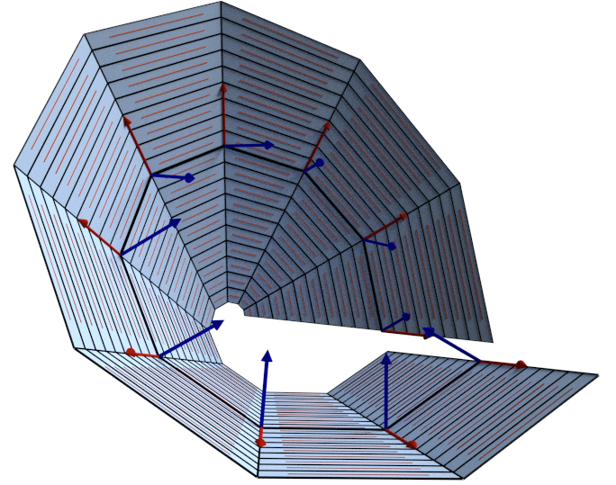
Surfaces of planar strips have been considered as discrete developable as they can obviously be unfolded into the plane [28]; such immersions correspond to developable curvature line edge-constraint nets, which are characterized by a discrete analogue of parallel framed curves [2] (for example see Figure 13 left):

A polygonal curve $\alpha$ with vertices $\alpha_{0},...,\alpha_{k}$ and two orthonormal vectors $(u_{0},n_{0})$ anchored at $\alpha_{0}$ extend to a unique discrete parallel frame along $\alpha$ ; simply reflect through the perpendicular bisector planes of each edge of $\alpha$ . ¹⁰¹⁰ 10 This discrete parallel frame can also be understood as being generated from rotations about the curve binormal since the composition of two reflections is a rotation. Then $u_{i+1}-u_{i}$ and $n_{i+1}-n_{i}$ are both parallel to $\alpha_{i+1}-\alpha_{i}$ for all $i=0,...,k-1$ . To extend the polygonal curve $\alpha$ to a developable edge-constraint net $(f,n)$ , fix a sampling $y_{j}$ of the real line and define $f:(i,j)\mapsto\alpha_{i}+y_{j}\,u_{i}$ with Gauß map $n_{i}$ . The resulting net $(f,n)$ is then in fact circular.

Conversely, for a surface $M$ built from a collection of planar strips with intersection lines $u$ one can find a discrete parallel framed curve $(\alpha,u,n)$ giving rise to a developable circular edge-constraint net whose immersion realizes $M$ : choose an initial point $\alpha_{0}$ on an initial line $u_{0}$ and a unit normal $n_{0}\perp u_{0}$ . The reflection property then gives rise to unique $\alpha$ and $n$ . It turns out that the curvature line is invariant to the initial choice of $n_{0}$ (it is always parallel to $\alpha$ ), while the mean curvature is not (which can be interpreted as extra information on how the developable surface locally bends).

Examples of developable edge-constraint nets that are not in curvature line parametrization arise from the associated family of the constant mean curvature discrete isothermic cylinder; this family contains the well known Schwarz Lantern [29] (see Figure 13 right) as an immersion with vertex normals that coincide with those of the smooth cylinder.

4 Towards a conformal perspective

In the smooth setting two conformal immersions for a manifold $M$ , $f,\tilde{f}:M\to{\mathbb{R}}^{3}\cong\textup{Im}\mathbb{H}$ , are said to be spin-equivalent if there exists a spin transformation $\lambda:M\to\mathbb{H}^{*}$ , such that $\textup{d}\tilde{f}=\bar{\lambda}\textup{d}f\lambda$ ; the surface normal $n$ transforms as $\tilde{n}=\lambda^{-1}n\lambda$ . Geometrically, spin transformations correspond to stretch rotations of the tangent plane at every point. Therefore, they are conformal mappings and for simply connected domains any two surfaces which are conformally equivalent are related via a spin transformation. Kamberov, Pedit, and Pinkall [26] showed using spin transformations that one can classify all Bonnet pairs on a simply connected domain. Bonnet pairs are immersed surfaces that have the same metric and mean curvature but are not rigid body motions of each other.

We can define a discrete spin transformation by ”stretch-rotating” the normal transport quaternions (Definition 37) of an edge-constraint net.

Definition 52 (Discrete Spin Transformation).

Let $(f,n)$ be an edge-constraint net with quad graph $\mathbb{G}$ . The spin transformation is a map $\lambda:\mathbb{G}\to\mathbb{H}^{*}$ which transforms $(f,n)$ to $(\tilde{f},\tilde{n})$ . The normal at each vertex and the normal transport quaternions transform by:

\tilde{n}=\lambda^{-1}n\lambda,\quad\tilde{\phi}=\bar{\lambda}\phi\lambda_{1},\quad\mathrm{and}\quad\tilde{\psi}=\bar{\lambda}\psi\lambda_{2}.

(61)

If the immersion of the spin transformed quadrilateral closes (i.e., $\tilde{\phi}+\tilde{\phi}_{2}+\tilde{\psi}+\tilde{\psi}_{1}$ is real) then one can construct a new edge-constraint net via

\tilde{f}_{1}-\tilde{f}=\Im\tilde{\phi}\quad\mathrm{and}\quad\tilde{f}_{2}-\tilde{f}=\Im\tilde{\psi}.

(62)

Proof.

The Gauß map $\tilde{n}$ is still unit length since conjugation by a quaternion corresponds to a global rotation, so lengths are preserved. The edge constraint is satisfied since for an arbitrary edge (here denoted as first lattice shifts) we have

\tilde{\phi}^{-1}\tilde{n}\tilde{\phi}=\lambda_{1}^{-1}\phi^{-1}\bar{\lambda}^{-1}\lambda^{-1}n\lambda\bar{\lambda}\phi\lambda_{1}=\lambda_{1}^{-1}\phi^{-1}n\phi\lambda_{1}=\lambda_{1}^{-1}(-n_{1})\lambda_{1}=-\tilde{n}_{1}.

(63)

∎

The spin transformation is invertible in the following sense, yielding a notion of discrete conformity.

Lemma 53.

If $(\tilde{f},\tilde{n})$ is a spin transform of $(f,n)$ with $\lambda$ then $(f,n)$ is a spin transformation of $(\tilde{f},\tilde{n})$ with $\lambda^{-1}$ .

Definition 54 (Discrete Conformal).

Two edge-constraint net quads are discretely conformally equivalent if they are spin-transformations of each other.

This spin transformation can give rise to edge-constraint net Bonnet pairs, an example is shown in Figure 14. The Darboux transformations of discrete isothermic nets [21] are also spin transformations, the proof is along the same lines as that of the following theorem.

Theorem 55.

The nets in the associated family of a discrete isothermic minimal net are conformal to each other.

Proof.

Perform the spin transformation with $\lambda=\cos(\frac{\alpha}{2})-\sin(\frac{\alpha}{2})n$ on the discrete isothermic minimal nets given by the Weierstrass representation (Definition 19) and see that one recovers the associated family edge (Definition 22). ∎

5 Lax pair edge-constraint nets

The language of moving frames combined with the theory of integrable systems offers a powerful tool with which to unify and systematically discretize parametrized surface theory for particular types of special parametrizations [9, 11]. We used this explicitly for showing that discrete isothermic constant mean curvature nets [33, 9, 23] and their associated families are constant mean curvature edge-constraint nets. Although not explicitly used here, K-nets and their associated families also possess algebraic formulations in this integrable framework [8, 7]. In general, this description is based on the existence of a Lax pair governing the structure equation of the surface—which can then be integrated via the Sym–Bobenko formula [5, 40]—or in the discrete case alternatively by the 3D consistency of the governing equation [11]. We now state a condition on Lax matrices (expressed as elements in the space of invertible quaternions $\mathbb{H}^{*}$ ) that guarantees the resulting nets will be edge-constraint. The condition is not very strong, and after an appropriate gauge transformation many discrete integrable systems related to surface theory exhibit such representations.

Theorem 56.

Let $\lambda(\alpha)$ be a spectral parameter depending on a real parameter $\alpha$ . Let $\Phi\in\mathbb{H}^{*}$ be a moving frame defined by shifts $\Phi_{1}:=U(\lambda)\Phi$ and $\Phi_{2}:=V(\lambda)\Phi$ (starting from a fixed $\Phi$ ), where $U(\lambda),V(\lambda)\in\mathbb{H}^{*}$ are the $\emph{Laxmatrices}$ satisfying the compatibility condition $V_{1}(\lambda)U(\lambda)=U_{2}(\lambda)V(\lambda)$ . Let $s\in{\mathbb{R}}$ be an arbitrary coefficient. Then the family of discrete contact element nets $(f^{\alpha},n^{\alpha})$ given by the Sym–Bobenko formula

$\displaystyle n^{\alpha}$	$\displaystyle:=$	$\displaystyle\Phi^{-1}\mathbbm{k}\Phi$
$\displaystyle\mathbbm{f}^{\alpha}$	$\displaystyle:=$	$\displaystyle s\,\Phi^{-1}\frac{d}{d\alpha}\Phi\|_{\lambda(\alpha)}+tn=s\Phi^{-1}\Phi_{\alpha}+tn,$	(64)
$\displaystyle f^{\alpha}$	$\displaystyle:=$	$\displaystyle\Im\mathbbm{f},$

for some $t\in{\mathbb{R}}$ are edge-constraint nets if and only if the Lax matrices $U(\lambda)$ and $V(\lambda)$ depend on $\lambda$ only in their off-diagonal entries. The edge-constraint is encoded in the relationships

n_{1}=-(\mathbbm{f}_{1}-\mathbbm{f})n(\mathbbm{f}_{1}-\mathbbm{f})^{-1}~\mathrm{and}~n_{2}=-(\mathbbm{f}_{2}-\mathbbm{f})n(\mathbbm{f}_{2}-\mathbbm{f})^{-1}.

(65)

Proof.

The proof is equivalent for both lattice directions, so we provide details for the first one, resulting in a condition on the $U(\lambda)$ Lax matrix: Up to a global rotation by $\Phi$ we find

$\displaystyle(\mathbbm{f}_{1}-\mathbbm{f})n$	$\displaystyle=$	$\displaystyle(s\,U^{-1}U_{\alpha}+t(U^{-1}\mathbbm{k}U-\mathbbm{k}))\mathbbm{k}$
	$\displaystyle=$	$\displaystyle U^{-1}(s\,U_{\alpha}+t(\mathbbm{k}U-U\mathbbm{k})\mathbbm{k}$
	$\displaystyle=$	$\displaystyle U^{-1}\left(s\,U_{\alpha}\mathbbm{k}+t(\mathbbm{k}U\mathbbm{k}+U)\right)$
	$\displaystyle=$	$\displaystyle U^{-1}\left(s\,U_{\alpha}\mathbbm{k}+t((-\mathbbm{k}U)(-\mathbbm{k})+(-\mathbbm{k}U)(-\mathbbm{k}U)^{-1}U)\right)$
	$\displaystyle\stackrel{{\scriptstyle!}}{{=}}$	$\displaystyle U^{-1}(-\mathbbm{k}U)(\mathbbm{f}_{1}-\mathbbm{f})$
	$\displaystyle=$	$\displaystyle-n_{1}(\mathbbm{f}_{1}-\mathbbm{f})$

precisely when:

U_{\alpha}\mathbbm{k}=-\mathbbm{k}U_{\alpha},

(66)

which is equivalent to $U$ having only off-diagonal entries dependent on $\lambda(\alpha)$ . ∎

6 Acknowledgements

We thank Julia Plehnert and Henrik Schumacher for helpful discussions, particularly with helping to resolve the definitions with a developable theory of edge-constraint nets.

Appendix A cK-net primer

Following [7] a Lax representation for K-nets is given by the $SU(2)$ matrices

\begin{array}[]{rcl}U&=&\left(\begin{array}[]{cc}\cot(\frac{\sigma_{u}}{2})\frac{H_{1}}{H}&i\lambda\\ i\lambda&\cot(\frac{\sigma_{u}}{2})\frac{H}{H_{1}}\end{array}\right)\\ V&=&\left(\begin{array}[]{cc}1&\frac{i}{\lambda}\tan(\frac{\sigma_{v}}{2})H_{2}H\\ \frac{i}{\lambda}\tan(\frac{\sigma_{v}}{2})\frac{1}{H_{2}H}&1\end{array}\right)\end{array}

(67)

depending on a (real) spectral parameter $\lambda$ with $H=e^{ih}$ for $h\in{\mathbb{R}}$ and the matrix problem

\Phi_{1}=U\Phi,\quad\Phi_{2}=V\Phi.

(68)

The integrability condition $V_{1}U=U_{2}V$ is then equivalent to $h$ solving the Hirota equation [22]

e^{i(h_{12}+h)}-e^{i(h_{1}+h_{2})}=\tan\frac{\sigma_{u}}{2}\tan\frac{\sigma_{v}}{2}\left(1-e^{i(h+h_{1}+h_{12}+h_{2})}\right).

(69)

Given the observation that the diagonals in K-nets satisfy the edge-constraint one can consider matrices

\mathcal{L}=V_{1}U=\left(\begin{array}[]{cc}\cot\frac{\delta}{2}\frac{H_{1}}{H}+\tan\frac{\delta}{2}H_{1}H_{12}&i(\lambda-\frac{HH_{12}}{\lambda})\\ i(\lambda-\frac{1}{\lambda HH_{12}})&\cot\frac{\delta}{2}\frac{H}{H_{1}}+\tan\frac{\delta}{2}\frac{1}{H_{1}H_{12}}\end{array}\right)

(70)

by choosing $\delta=\sigma_{u}=-\sigma_{v}$ . Setting aside the fact that $\mathcal{L}$ arises as the product of two matrices along edges of a K-net, we can investigate the compatability condition for $\mathcal{L}$ assigned to edges of a lattice. After relabeling the entries we have

\begin{array}[]{rcl}L&=&\left(\begin{array}[]{cc}\cot\frac{\delta_{1}}{2}\frac{l}{s}+\tan\frac{\delta_{1}}{2}ls_{1}&i(\lambda-\frac{ss_{1}}{\lambda})\\ i(\lambda-\frac{1}{\lambda ss_{1}})&\cot\frac{\delta_{1}}{2}\frac{s}{l}+\tan\frac{\delta_{1}}{2}\frac{1}{ls_{1}}\end{array}\right)\\ M&=&\left(\begin{array}[]{cc}\cot\frac{\delta_{2}}{2}\frac{m}{s}+\tan\frac{\delta_{2}}{2}ms_{2}&i(\lambda-\frac{ss_{2}}{\lambda})\\ i(\lambda-\frac{1}{\lambda ss_{2}})&\cot\frac{\delta_{2}}{2}\frac{s}{m}+\tan\frac{\delta_{2}}{2}\frac{1}{ms_{2}}\end{array}\right)\end{array}

(71)

with unitary variables $s$ at vertices of a square lattice and $l$ and $m$ on edges in first and second lattice directions. The compatibility condition

M_{1}L=L_{2}M

(72)

implies $\det M_{1}\det L=\det L_{2}\det M$ and in the spirit of the K-net case we thus assume $\delta_{1}$ is constant in the second lattice direction and $\delta_{2}$ is constant in the first one. Then Equation (72) can be solved, i.e., given $s,s_{1},s_{2},l,m,\delta_{1}$ , and $\delta_{2}$ then $m_{1},l_{2},$ and $s_{12}$ are uniquely determined. However, in order to be able to have arbitrary edge lengths for the resulting net, one needs to allow for $\sin\delta_{i}>1$ and thus complex $\delta_{i}$ . To keep $L$ and $M$ quaternionic $l$ and $m$ will no longer be unitary but have absolute value

\sqrt{\frac{\cos\left(\rho_{i}-\arg\tan\frac{\delta_{i}}{2}\right)+\cos\left(\rho-\arg\tan\frac{\delta_{i}}{2}\right)}{\cos\left(\rho_{i}+\arg\tan\frac{\delta_{i}}{2}\right)+\cos\left(\rho+\arg\tan\frac{\delta_{i}}{2}\right)}}

(73)

where $s=e^{i\rho}$ .

Theorem 57.

Let $\Phi:{\mathbb{Z}}^{2}\to{\mathbb{R}}^{3}$ be a solution to $\Phi_{1}=L\Phi$ , $\Phi_{2}=M\Phi$ with $L$ and $M$ as in Equation (71) solving the integrability condition Equation (72). Then $f:{\mathbb{Z}}^{2}\to{\mathbb{R}}^{3}$ and $n:{\mathbb{Z}}^{2}\to{\mathbb{S}^{2}}$ given by

f=2\Phi^{-1}\frac{\partial}{\partial t}\Phi~\mathrm{and}~n=\Phi^{-1}\mathbbm{k}\Phi

(74)

is an edge-constraint net of Gauß curvature $K=-1$ . If $\lambda=1$ , $f$ is circular. Moreover any circular edge-constraint quadrilateral with parallel normals and $K=-1$ can be generated this way.

Proof.

Circularity in the case of $\lambda=1$ and the Gauß curvature $K=-1$ for any real $\lambda$ can be computed directly. To see that every quadrilateral arises this way, one can show that the quad with its normals is uniquely defined by three vertices and a normal. However this is exactly the initial data one prescribes for the compatibility condition of the Lax pair. Since both problems have a unique solution they must coincide. ∎

References

[1] L. Bianchi. Lezioni di geometria differenziale, volume 1-2. Spoerri, Pisa, seconda edizione, riveduta e cosiderevolmente aumentata edition, 1902.
[2] R. L. Bishop. There is more than one way to frame a curve. American Mathematical Monthly, pages 246–251, 1975.
[3] A. Bobenko, U. Hertrich-Jeromin, and I. Lukyanenko. Discrete constant mean curvature nets in space forms: Steiner’s formula and Christoffel duality. Discrete and Computational Geometry, 52(4):612–629–629, 2014.
[4] A. I. Bobenko. All constant mean curvature tori in R 3, S 3, H 3 in terms of theta-functions. Mathematische Annalen, 290(1):209–245, 1991.
[5] A. I. Bobenko. Surfaces in terms of 2 by 2 matrices: Old and new integrable cases. In A. P. Fordy and J. C. Wood, editors, Harmonic maps and integrable systems, pages 83–129. Vieweg, Braunschweig/Wiesbaden, 1994.
[6] A. I. Bobenko. Surfaces from Circles. In A. I. Bobenko, J. M. Sullivan, P. Schröder, and G. M. Ziegler, editors, Oberwolfach Seminars, pages 3–35. Birkhäuser Basel, 2008.
[7] A. I. Bobenko and U. Pinkall. Discrete surfaces with constant negative Gaussian curvature and the Hirota equation. Journal of Differential Geometry, 43:527–611, 1996a.
[8] A. I. Bobenko and U. Pinkall. Discrete isothermic surfaces. Journal für die reine und angewandte Mathematik, pages 187–208, 1996b.
[9] A. I. Bobenko and U. Pinkall. Discretization of Surfaces and Integrable Systems. In A. I. Bobenko and R. Seiler, editors, Discrete integrable geometry and physics, pages 3–58. Oxford University Press, 1999.
[10] A. I. Bobenko and R. Seiler. Discrete integrable geometry and physics. Oxford Lecture Series in Mathematics and Its Applications. Oxford University Press, 1999.
[11] A. I. Bobenko and Y. B. Suris. Discrete Differential Geometry: Integrable Structure, volume 98 of Graduate Studies in Mathematics. American Mathematical Society, 2008.
[12] A. I. Bobenko and Y. B. Suris. Discrete Koenigs nets and discrete isothermic surfaces. International Mathematics Research Notices, 2009(11):1976–2012, 2009.
[13] A. I. Bobenko, T. Hoffmann, and B. A. Springborn. Minimal Surfaces from Circle Patterns: Geometry from Combinatorics. Annals of Mathematics, 164(1):pp. 231–264, 2006.
[14] A. I. Bobenko, J. M. Sullivan, P. Schröder, and G. M. Ziegler. Discrete Differential Geometry, volume 38 of Oberwolfach Seminars. Springer, 2008.
[15] A. I. Bobenko, H. Pottmann, and J. Wallner. A curvature theory for discrete surfaces based on mesh parallelity. Mathematische Annalen, 348(1):1–24, 2010.
[16] F. Burstall, U. Hertrich-Jeromin, and W. Rossman. Discrete linear Weingarten surfaces. arXiv preprint arXiv:1406.1293, 2014a.
[17] F. Burstall, U. Hertrich-Jeromin, W. Rossman, and S. Santos. Discrete special isothermic surfaces. Geometriae Dedicata, pages 1–11, 2014b.
[18] J. Cieśliński, A. Doliwa, and P. M. Santini. The integrable discrete analogues of orthogonal coordinate systems are multi-dimensional circular lattices. Physics Letters A, 235(5):480–488, 1997.
[19] G. Darboux. Leçons sur la théorie générale des surfaces et les applications géometriques du calcul infinitésimal. Paris Gauthier-Villars, 1887.
[20] J. Dorfmeister, F. Pedit, and H. Wu. Weierstrass type representation of harmonic maps into symmetric spaces. Communications and Analysis of Geometry, 6:633–668, 1998.
[21] U. Hertrich-Jeromin, T. Hoffmann, and U. Pinkall. A discrete version of the Darboux transform for isothermic surfaces. In A. I. Bobenko and R. Seiler, editors, Discrete integrable geometry and physics, pages 59–81. Oxford University Press, 1999.
[22] R. Hirota. Nonlinear partial difference equations III; Discrete sine-Gordon equation. Journal of the Physical Society of Japan, 43(6):2079–2086, 1977.
[23] T. Hoffmann. Discrete CMC surfaces and discrete holomorphic maps. In A. I. Bobenko and R. Seiler, editors, Discrete integrable geometry and physics, pages 97–112. Oxford University Press, 1999a.
[24] T. Hoffmann. Discrete Amsler surfaces and a discrete Painlevé III equation. In A. I. Bobenko and R. Seiler, editors, Discrete integrable geometry and physics, pages 83–96. Oxford University Press, 1999b.
[25] T. Hoffmann. Discrete Hashimoto surfaces and a doubly discrete smoke-ring flow. In A. I. Bobenko, J. M. Sullivan, P. Schröder, and G. M. Ziegler, editors, Discrete Differential Geometry, pages 95–115. Springer, 2008.
[26] G. Kamberov, F. Pedit, and U. Pinkall. Bonnet pairs and isothermic surfaces. Duke Mathematical Journal, 92(3):637–644, 1998.
[27] B. G. Konopelchenko and W. K. Schief. Trapezoidal discrete surfaces: geometry and integrability. Journal of Geometry and Physics, 31(2):75–95, 1999.
[28] Y. Liu, H. Pottmann, J. Wallner, Y.-L. Yang, and W. Wang. Geometric modeling with conical meshes and developable surfaces. ACM Transactions on Graphics, 25(3):681–689, 2006.
[29] J.-M. Morvan. Generalized Curvatures, volume 2 of Geometry and Computing. Springer Berlin Heidelberg, 2008.
[30] J. J. C. Nimmo and W. K. Schief. Superposition principles associated with the Moutard transformation: an integrable discretization of a (2+1)-dimensional sine-Gordon system. Proceedings of the Royal Society A: Mathematical, Physical and Engineering Sciences, 453(1957):255–279, 1997.
[31] A. W. Nutbourne and R. R. Martin. Differential geometry applied to curve and surface design, volume 1. Horwood Chichester, 1988.
[32] J. Oprea. The mathematics of soap films: Explorations with Maple, volume 10 of Student Mathematical Library. American Mathematical Society, 2000.
[33] F. Pedit and H. Wu. Discretizing constant curvature surfaces via loop group factorizations: the discrete sine-and sinh-Gordon equations. Journal of Geometry and Physics, 17(3):245–260, 1995.
[34] U. Pinkall. Designing cylinders with constant negative curvature. In A. I. Bobenko, P. Schröder, J. M. Sullivan, and G. M. Ziegler, editors, Discrete Differential Geometry, pages 57–66. Springer, 2008.
[35] U. Pinkall and I. Sterling. On the classification of constant mean curvature tori. Annals of Mathematics, pages 407–451, 1989.
[36] U. Pinkall, B. Springborn, and S. Weißmann. A new doubly discrete analogue of smoke ring flow and the real time simulation of fluid flow. Journal of Physics A: Mathematical and Theoretical, 40(42):12563, 2007.
[37] R. Sauer. Parallelogrammgitter als Modelle pseudosphärischer Flächen. Mathematische Zeitschrift, 52(1):611–622, 1950.
[38] R. Sauer. Differenzengeometrie. Springer Verlag, 1970.
[39] W. K. Schief. On a maximum principle for minimal surfaces and their integrable discrete counterparts. Journal of Geometry and Physics, 56(9):1484–1495, 2006.
[40] A. Sym. Soliton surfaces and their applications (soliton geometry from spectral problems). In R. Martini, editor, Lecture Notes in Physics, pages 154–231. Springer Berlin Heidelberg, 1985.
[41] S. Tabachnikov and E. Tsukerman. On the discrete bicycle transformation. Publicaciones matematicas del Uruguary (proceedings of the Montevideo Dynamical Systems Congress 2012), 14:201–220, 2013.
[42] W. Wunderlich. Zur Differenzengeometrie der Flächen konstanter negativer Krümmung. Springer Verlag, 1951.

A discrete parametrized surface theory in ℝ3{\mathbb{R}}^{3}

Abstract

1 Introduction

2 Edge-constraint nets

2.1 Setup

Definition 1 (Quadrilateral net).

Remark (Shift notation).

Definition 2 (Edge-constraint net).

Remark.

Lemma 3.

Proof.

Lemma 4.

Lemma 5 (Offset nets).

2.2 Curvatures from Offsets

Definition 6 (Mixed area form).

Remark.

Theorem 7 (Steiner formula).

Definition 8.

Remark (Degenerate Gauß maps).

Definition 9 (Edge-constraint curvatures).

Remark (Degenerate immersions).

Remark (Sign of projection direction).

Remark (Choice of partial derivatives).

Definition 10 (Fundamental forms).

Lemma 11.

Proof.

Lemma 12 (Curvature and fundamental form relationships).

Example (Spherical edge-constraint nets).

Example (Curvature line fields).

3 Constant Curvature Nets

3.1 Discrete minimal surfaces

Definition 13 (Minimal edge-constraint net).

Definition 14 (Circular net).

Lemma 15.

Proof.

Definition 16 (Isothermic net).

Lemma 17.

Definition 18.

Definition 19 (Weierstrass representation of discrete isothermic minimal nets).

Lemma 20.

Proof.

Lemma 21.

Proof.

Definition 22 (Associated family of discrete isothermic minimal net).

Lemma 23.

Proof.

Lemma 24.

Proof.

Lemma 25 (Quad geometry of the associated family).

Proof.

Theorem 26 (Minimality of the associated family).

Proof.

Theorem 27 (Gauß curvature of the associated family).

Proof.

Definition 28 (Discrete asymptotic net).

Lemma 29.

Proof.

Lemma 30.

Proof.

3.2 Discrete constant mean curvature surfaces

Definition 31 (Constant mean curvature edge-constraint net).

Lemma 32 (Linear Weingarten relationship).

Proof.

Corollary 33.

Remark.

Lemma 34.

Definition 35 (Associated family).

Lemma 36.

Proof.

Definition 37 (Normal transport quaternions).

Lemma 38 (Edge-constraint as a skew parallelogram).

Definition 39.

Lemma 40.

Proof.

Theorem 41 (Darboux transform for parallelograms).

Proof.

Theorem 42.

Proof.

Remark.

Theorem 43.

A discrete parametrized surface theory in ${\mathbb{R}}^{3}$