A trajectory-free framework for analysing multiscale systemsThanks: This project was funded by the Australian Research Council Grant DP120104514.

Effective numerical simulation of multiscale systems constitutes a formidable challenge. Consider a system which has slow dynamics on a time-scale of order one and fast dynamics on the scale of order $1/\epsilon$ for some parameter $\epsilon\ll 1$. In molecular dynamics, for example, the time-scale separation can be of the order of $\epsilon\approx 10^{-14}$ [6]. To accurately simulate orbits numerically and to assure numerical stability, the time step of the integrator must be of the order of $\epsilon$. To capture the relevant slow dynamics a total number of integration steps of the order of $1/\epsilon$ is required, making direct numerical simulations of orbits computationally impractical.

Numerical integrators are subject to two main sources of error. The first is truncation error, which is the inability of the numerical method (Runge–Kutta, Euler–Maruyama, etc.) to fully capture the actual dynamics of the system. The second is round-off error, due to implementing the numerical method on a computer with finite precision arithmetic. While truncation error decreases with a smaller time step, round-off error increases [16, 13]. In a multiscale system, if the time-scale separation is large, it may be impossible to find a time step which is simultaneously small enough to avoid significant truncation error for the fast dynamics and sufficiently large to avoid detrimental accumulation of round-off error for the slow dynamics.

Even if orbits could be computed exactly, analysing a multiscale system using a time series extracted from a true orbit can still yield incorrect data about the diffusion process of the slow variables [18]. To avoid this problem, the time series must be sampled at a rate intermediate between the slow and fast variables and these rates might not be known in advance.

There exists a variety of numerical methods dealing with one or more aspects of these numerical difficulties (see [6] and references therein). These methods rely on producing trajectories of the dynamical system via some form of time-integration with some of the issues mentioned above remaining. In this paper, we develop algorithms which avoid trajectory integration altogether. Besides the advantages relating to the issues of time-integration mentioned above, the algorithm allows for a huge reduction in computational time. Our main objective is to develop numerical algorithms which, given a dynamical system,

1. 1.

   test whether the system exhibits multiscale behaviour, and if so

2. 2.

   determine the order of the time-scale separation, and then

3. 3.

   construct effective reduced equations for the slow dynamics allowing for the application of large time steps.

The framework we adopt for this integration-free approach is based on the infinitesimal generator associated to the underlying continuous-time dynamical system. In Section 2 we briefly review the notion of generators of transfer and Koopman operators. Section 3 introduces a trajectory-free test for multiscale behaviour. The degree of time-scale separation is estimated in algorithms described in Sections 4 and 5. A method to determine the reduced slow dynamics from a multiscale system without relying on statistics obtained from long time-integrations is given in Section 6. The algorithms are tested in numerical simulations in Section 7. We conclude with a discussion in Section 8.

We describe our methodology for Itō drift-diffusion processes, as these are a large and flexible class of dynamical systems, and the spectral properties of the corresponding transfer operators are relatively straightforward. Consider a drift-diffusion process

defined on a subset $\mathcal{Z}$ of $\mathbb{R}^{d}$ where $l\leq d$ and each $W_{k}$ for $k=1,\ldots,\ell$ represents an independent Wiener process. Given a probability density function at time $t=0$, the density at future times is determined by the Fokker–Planck equation

where

The second order differential operator $\mathcal{L}$ is called the Fokker–Planck operator. At each point $z$ in the phase space $\mathcal{Z}$, the vector $\mu(z)\in\mathbb{R}^{d}$ represents the drift of the process and the positive semi-definite matrix $D(z)=\sigma(z)\sigma(z)^{\top}\in\mathbb{R}^{d\times d}$ the diffusion. The operator $\mathcal{L}$ generates a family of operators $e^{t\mathcal{L}}$ for $t\geq 0$ such that $e^{s\mathcal{L}}e^{t\mathcal{L}}=e^{(s+t)\mathcal{L}}$ and $\lim_{t\to 0}\tfrac{1}{t}[e^{t\mathcal{L}}-Id]=\mathcal{L}$. If $\rho\in L^{1}(\mathcal{Z})$ is an initial probability density, then $e^{t\mathcal{L}}(\rho)$ is the density after time $t$. Thus, $e^{t\mathcal{L}}$ may be thought of as a transfer operator defined on $L^{1}(\mathcal{Z})$. Since the underlying system is a random dynamical system and $e^{t\mathcal{L}}$ represents an average over all possible random paths, it is an annealed transfer operator [1].

In many cases, the Fokker–Planck operator has compact resolvent [15]. In particular, its spectrum consists of a countable set of eigenvalues $\{\lambda_{k}\}_{k=0}^{\infty}$ which, when ordered by the convention

satisfy $\lim_{k\to\infty}\operatorname{Re}\lambda_{k}\to-\infty$. As a consequence, for each $t>0$ the operator $e^{t\mathcal{L}}$ is compact with eigenvalues $e^{t\lambda_{k}}$ tending to zero as $k\to\infty$. The invariant density $\rho_{0}$ of the system is an eigenfunction of $\mathcal{L}$ associated to the eigenvalue $\lambda_{0}=0$.

The Kolmogorov backward equation is given by $\tfrac{\partial f}{\partial t}=\mathcal{L}^{*}f$ where the adjoint of the Fokker–Planck operator is given by

This adjoint operator generates a family of operators $K_{t}:=e^{t\mathcal{L}^{*}}=(e^{t\mathcal{L}})^{*}$ for $t\geq 0$. If $f\in L^{\infty}(\mathcal{Z})$, then $K_{t}(f)\in L^{\infty}(\mathcal{Z})$ is given by $K_{t}(f)(z)=\mathbb{E}f(\zeta(t))$ where the expectation is over all paths $\zeta(t)$ in the drift-diffusion process which satisfy $\zeta(0)=z$. The operator $K_{t}$ may therefore be regarded as an annealed Koopman or composition operator.

The operators $\mathcal{L}^{*}$ and $\mathcal{L}$ share the same eigenvalues $\lambda_{k}$. Consider the eigenfunction $\psi_{k}\in L^{\infty}(\mathcal{Z})$ of $\mathcal{L}^{*}$ associated to $\lambda_{k}$. This function $\psi_{k}$ is an observable which evolves according to

and therefore decays to zero at the rate given by $|e^{t\lambda_{k}}|$ for $t>0$. In general, the eigenfunctions of $\mathcal{L}^{*}$ associated to eigenvalues with real part closest to zero are the observables of the system which decay at the slowest speeds possible. The eigenvalues $\lambda_{k}$ for small $k$ therefore correspond to speed of the slowest dynamics present in the system. These ideas have been exploited to identify almost-invariant sets [5, 9, 7] for deterministic and annealed random dynamics, and coherent sets [10] for quenched random or time-dependent dynamics.

Suppose that the system under study is a multiscale system. That is, assume there is a value $0<\epsilon\ll 1$ representing the time-scale separation and transverse directions of fast and slow dynamics such that the components of the drift and diffusion are on the order of $O(\epsilon^{-1})$ in the fast direction and $O(1)$ in the slow direction. Further suppose that $\lambda_{k}$ is an eigenvalue of $\mathcal{L}^{*}$ such that $|\operatorname{Re}\lambda_{k}|\ll\epsilon^{-1}$. Then, one may choose an intermediate time $t\gg\epsilon$ such that

Since $t\gg\epsilon$, the system after time $t$ has evolved towards equilibrium in the fast dynamics implying that $K_{t}\psi_{k}$ is nearly constant along the direction of the fast dynamics. Therefore, $\psi_{k}$ should be approximately constant in this direction as well. This observation is developed in more detail in [3, 8].

Given the ordering in (3), we refer to the eigenvalues $\lambda_{k}$ for small $k$ (and therefore small $|\operatorname{Re}\lambda_{k}|$) as the leading eigenvalues with the associated leading eigenfunctions $\psi_{k}$ . By the above observations, in a multiscale system, the level sets of a leading eigenfunction $\psi_{k}$ closely approximate fast fibres, submanifolds of the system along which the fast dynamics occurs. This property is used in the following sections to develop algorithms which test for multiscale behaviour.

We now use these properties of the Fokker–Planck operator and its adjoint to develop an algorithm to test for multiscale behaviour. We focus on the case of stochastic differential equations (SDEs) where the slow dynamics is one-dimensional. The only information used by the algorithm are functions $\mu$ and $D$ defining the drift and diffusion of the process. In particular, we do not assume any a priori knowledge of the slow or fast directions (if they exist) or that these directions align with the coordinates in which the system is defined. We first outline the idea behind the algorithm before providing the actual algorithm.

As established in the previous section, the level sets of the leading eigenfunctions $\psi_{k}$ of the adjoint Fokker-Planck operator $\mathcal{L}^{*}$ contain information about the multi-scale behaviour of the dynamics. If the system has multiscale behaviour, these level sets will approximate a fast fibre of the system. We use the eigenfunction $\psi_{1}$ and numerically compute a fibre $F$ as a connected component of a level set $\psi_{1}^{-1}(\{s\})$ (cf. step 3 in Algorithm 1). If the leading eigenfunctions are complex valued, we may choose without loss of generality the real (or imaginary) part of the eigenfunctions to define the fibres (in Section 7 we will give such an example). There is a significant history of computing eigenfunctions of the Fokker–Planck operator or its adjoint numerically [2, 9] which we will employ to determine eigenfunctions $\psi_{k}$ of $\mathcal{L}^{*}$ associated to the eigenvalues $\lambda_{k}$ for small $k$ (cf. step 2 in Algorithm 1).

If the system actually exhibits multiscale dynamics and the fibre $F$ approximates a fast fibre, then the speed of the dynamics will be much faster along the fibre than transverse to it. Therefore, one expects in this case that the drift and the diffusion along one or both of the averages tangent to the fibre $F$ will be significantly larger than those corresponding to the direction normal to $F$. We therefore calculate the drift and diffusion coefficients for a set of points on the fibre $F$ and then subsequently use their averages along the fibre to probe for fast dynamics along the fibre and slow dynamics transverse to the fibre (this is achieved in steps 4 and 5 of Algorithm 1, respectively).

Computing the drift and diffusion coefficients $\mu^{\text{nor}}(z)$, $\mu^{\text{tan}}(z)$, $D^{\text{nor}}(z)$, and $D^{\text{tan}}(z)$ normal and tangent to the fibre at a finite set of points $Q$ uniformly distributed over $F$ constitutes the most complicated step of the algorithm and is explained in further detail below in Subsection 3.1.

The most natural way to compute the averages of the drift and diffusion coefficients $\mu^{\text{nor}}(z)$, $\mu^{\text{tan}}(z)$, $D^{\text{nor}}(z)$, and $D^{\text{tan}}(z)$ along the fibre is using the invariant density along the fibre. As an approximation for the invariant density of the fast dynamics on the fibre, we use the invariant density function $\rho_{0}$ of the full multi-scale system and simply restrict $\rho_{0}$ to $F$. The property that $\rho_{0}$ is invariant is equivalent to $\mathcal{L}\rho_{0}=0$. Therefore, we estimate $\rho_{0}$ by solving numerically for the eigenfunction of $\mathcal{L}$ whose associated eigenvalue is closest to zero (cf. step 1 of Algorithm 1). The measure on $F$ can be approximated by a measure supported on a finite set. We choose a finite set of points $Q$ uniformly distributed over $F$ and define weights $w_{z}\in\mathbb{R}$ such that $\sum_{z\in Q}w_{z}\delta_{z}$ approximates the density $\rho_{0}$ on $F$. Here, $\delta_{z}$ is the Dirac measure at $z$ and $w_{z}:=c\rho_{0}(z)$ where the scaling constant $c$ is defined such that $\sum_{z\in Q}w_{z}=1$ (cf. step 4 of Algorithm 1).

As a criterion for the presence or absence of multi-scale behaviour we then compare the averages along the fibre of the absolute values of the normal and tangential drift and diffusion coefficients; if the tangential components are much larger than the perspective normal ones, this is indicative of $F$ being a fast fibre and the system exhibiting multi-scale behaviour (cf. step 7).

We now propose a further test for multiscale behaviour which also estimates the magnitude of the time-scale separation between the slow and fast dynamics. This estimation is achieved by comparing the spectrum of the operator $\mathcal{L}$ on the full system to the spectrum of an operator defined by dynamics along the fibre $F$.

Recall from Section 2 that the leading eigenvalues of $\mathcal{L}$ (which are the same as those of its adjoint $\mathcal{L}^{*}$) correspond to the slowest rates of decay for observables under the dynamics of the system. Therefore, they give an estimate of the speed of the slow dynamics which can be computed from the full system.

We now define a Fokker–Planck operator ${\widehat{\mathcal{L}}}_{\text{tan}}$ for the dynamics tangent to the fast fibre $F$. For a multiscale system, the dynamics associated to ${\widehat{\mathcal{L}}}_{\text{tan}}$ is entirely fast and does not capture any of the slow dynamics. Therefore, its leading eigenvalues $\widehat{\lambda}_{k}$ correspond to the speed of the fast dynamics alone.

We are assuming that the slow dynamics evolves on a time-scale of $O(1)$ and the fast dynamics on a time-scale of $O(1/\epsilon)$ for some unknown value $\epsilon$. The leading eigenfunctions $\psi_{k}$ of $\mathcal{L}^{*}$ are observables which decay to zero at the rate of the slow dynamics of the systems. Because of this, the real part of the associated eigenvalues $\lambda_{k}$ are $O(1)$. The leading eigenfunctions of ${\widehat{\mathcal{L}}}_{\text{tan}}^{*}$ are observables along the fibre $F$ which decay at a speed associated to the fast dynamics and so the associated eigenvalues $\widehat{\lambda}_{k}$ are $O(1/\epsilon)$. The ratio of the real parts of the leading $\lambda_{k}$ and the leading $\widehat{\lambda}_{k}$ then gives a quantitative estimate of the time-scale separation between the slow and fast variables. See also the discussion in [3, 8].

We now give an algorithm for determining these values $\widehat{\lambda}_{k}$ numerically. Let $F$ be a fibre as computed in Algorithm 1. Further suppose that $F$ is such that it can be represented globally as the graph of a function. That is, after a linear change of coordinates $A:\mathbb{R}^{d}\to\mathbb{R}^{d}$, the image $A(F)$ is equal to the set $\{(v,g(v)):v\in V\}$ for some function $g:V\to\mathbb{R}$ defined on a subset $V$ of $\mathbb{R}^{d-1}$. One may then define a drift-diffusion process on $V$ where the drift and diffusion components are given by $\hat{\mu}_{i}$ and $\hat{D}_{ij}$ for $1\leq i,j\leq d-1$ as defined in the previous section. Using this data, the leading eigenvalues $\widehat{\lambda}_{k}$ for the operator ${\widehat{\mathcal{L}}}_{\text{tan}}$ may be computed numerically.

We summarise the algorithm for the estimation of the time-scale separation as

Ideally, Algorithms 1 and 2A should both be performed on a given system to test for multiscale behaviour. Algorithm 1 tests that on a fibre $F$ the tangent components of the drift and diffusion dominate the normal components. Therefore, it justifies approximating the fast dynamics by a drift-diffusion process restricted to the fibre and defined purely by these tangent components. Algorithm 2A then uses the eigenvalues of the resulting operator ${\widehat{\mathcal{L}}}_{\text{tan}}$ associated to this process in order to estimate the speed of the dynamics restricted to the fibre.

Algorithm 2A assumes that the fibre $F$ can be expressed globally as the graph of a function. If the shape of $F$ is such that finding a graph is not possible, then one could instead estimate these eigenvalues by using methods of trajectory integration and projection to the fibre as described in [8]. This alternative method does not follow the general trajectory-free framework proposed in this work. It may therefore be slower in general and subject to the concerns listed in the introduction. In the next section, we give a variant of Algorithm 2A which is always applicable in the specific case where the slow and fast directions are one-dimensional.

In the case that the fast fibre is one-dimensional (and the full system is therefore two-dimensional), an alternative to expressing the fibre as a graph is to parameterize the fibre by arc length. This is always possible, as topologically a one-dimensional fibre $F$ will either be a line or a circle.

Given a representation of the curve $F$, compute a sequence of points $\{q_{n}\}$ such that each point is at a uniform distance from the previous. To analyse the drift and diffusion at $q_{n}$, first approximate the tangent to the curve at $q_{n}$ by the vector $q_{n+1}-q_{n-1}$. Apply a rotation $A:\mathbb{R}^{2}\to\mathbb{R}^{2}$ such that $A(q_{n+1}-q_{n-1})$ is roughly horizontal. Writing $(v_{n},y_{n})=A(q_{n})$, apply a regression method to find a polynomial $p_{g}$ such that $y_{m}\approx p_{g}(v_{m})$ for points $(v_{m},y_{m})$ near $(v_{n},y_{n})$. By adjusting the angle of the rotation $A$, one may further assume that the first derivative $p_{g}^{\prime}$ satisfies $p_{g}^{\prime}(v_{n})=0$. Using the rotation $A$ composed with the change of coordinates mapping $(v,y)$ to $(v,y-p_{g}(v))$ compute the drift and diffusion data tangent and normal to the curve. Applying (5)–(9) in this specific case and using that $p_{g}^{\prime}(v_{n})=0$, the resulting coefficients are

For $v>v_{n}$ the arc length of the graph $\{(u,p_{g}(u)):u\in[v_{n},v]\}$ is given by

Using $p_{g}^{\prime}(v_{n})=0$, the first and second derivatives satisfy

If we take the derivative of $v$ with respect to itself, then

as well. This implies that two different parameterizations of the curve—one by arc length and the other by $v$—agree up to second order at $v_{n}$. Therefore, the Fokker–Planck operators coincide for the two parameterizations with the same drift and diffusion coefficients at the point $(v_{n},y_{n})$. Using this data, one can find for any point on $F$ the components tangent to the curve. One can therefore define a drift-diffusion process on the curve $F$ as parametrized by arc length and numerically compute the leading eigenvalues of the corresponding Fokker–Planck operator as before.

We present this as a variant of Algorithm 2A to estimate the time-scale separation:

Once the existence of multiscale dynamics has been established, one further step is to compute the reduced slow dynamics. We give here a simple technique to perform the reduction to a lower dimensional SDE. As with the other methods developed in this paper, the algorithm does not rely on trajectory integration.

First, consider a multiscale system where model reduction is applicable. That is, following the formalism given in [11, 8], there is a projection $\mathcal{P}:\mathcal{Z}\to\mathcal{X}$ from the domain of the full system $\mathcal{Z}$ to a smaller dimensional space $\mathcal{X}$ and an SDE on $\mathcal{X}$ such that orbits of the reduced system on $\mathcal{X}$ resemble projected orbits of the full system. Our goal is to reconstruct this reduced dynamics.

As before, let $\mathcal{L}$ denote the Fokker–Planck operator for the full SDE on $\mathcal{Z}$ and let $(\lambda_{k},\psi_{k})$ be the eigenpairs for the adjoint $\mathcal{L}^{*}$. For ease of notation, we assume here that all eigenvalues are simple. Similar reasoning holds in the more general case. Let $\tilde{\mathcal{L}}$ denote the Fokker–Planck operator for the reduced SDE on $\mathcal{X}$ and let $(\tilde{\lambda}_{k},\tilde{\psi}_{k})$ be the eigenpairs of $\tilde{\mathcal{L}}^{*}$. Assume both sequences are indexed by decreasing real part as in (3).

Recall that the leading eigenvalues $\lambda_{k}$ of $\mathcal{L}^{*}$ are associated to the speed of the slow dynamics and the eigenfunctions $\psi_{k}$ are approximately constant along fast fibres. In fact, using operator approximation theory, one may show that for $\epsilon$ sufficiently small, the approximations $\lambda_{k}\approx\tilde{\lambda}_{k}$ and $\psi_{k}\approx\tilde{\psi}_{k}\circ\mathcal{P}$ hold [3].

Suppose $C\subset\mathcal{Z}$ is a smooth curve transverse to the fast fibre which intersects each fibre exactly once. Define a projection $P_{c}:\mathcal{Z}\to C$ by letting $P_{c}(z)$ be the unique point on $C$ which is on the same fast fibre as $x$. Then $C$ may be identified with $\mathcal{X}$ and $P_{c}$ with $\mathcal{P}$. The above approximations then imply that $(\lambda_{k},\psi_{k}|_{C})$ is an approximation of the eigenpair $(\tilde{\lambda}_{k},\tilde{\psi}_{k})$. Moreover, the objects $\lambda_{k}$, $\psi_{k}$, and $C$ can all be computed numerically from the operator $\mathcal{L}^{*}$ for the full system. This means that even though we have no direct way of representing the operator $\tilde{\mathcal{L}}^{*}$ associated to the reduced dynamics on $\mathcal{X}$, we still have an indirect method of computing its leading eigenpairs.

There are a number of techniques for reconstructing the drift and diffusion of a system from its spectral data. For instance, see the survey [14] and more recent work in [4, 3]. We use a method attributed in [14] to S. G. Demoura. Let $\tilde{\mu}$ and $\tilde{D}$ be the (as yet unknown) coefficients of the drift and diffusion for the reduced SDE on $C$. Consider the formula (4) for the adjoint of the Fokker–Planck operator in the one-dimensional setting along the curve $C$. One sees that each eigenpair $(\tilde{\lambda}_{k},\tilde{\psi}_{k})$ of $\tilde{\mathcal{L}}^{*}$ satisfies the equation

where the prime denotes derivatives along the curve $C$. Using $\psi_{k}|_{C}$ as an approximation for $\tilde{\psi}_{k}$, one may estimate the derivatives $\tilde{\psi}_{k}^{\prime}$ and $\tilde{\psi}_{k}^{\prime\prime}$ numerically. By considering (10) for two distinct eigenpairs, say $(\tilde{\lambda}_{1},\tilde{\psi}_{1})$ and $(\tilde{\lambda}_{2},\tilde{\psi}_{2})$, one may solve the linear system of equations

pointwise along $C$ in order to solve for the drift $\tilde{\mu}$ and diffusion $\tilde{D}$ of the reduced system.

This technique requires an accurate estimate of the first and second derivatives of the eigenfunctions. In some settings, accurate derivative estimation is not possible and more sophisticated techniques must be applied, such as solving a quadratic programming problem based on the eigenfunction equations [12, 4, 3].

We now apply these techniques to an example studied in [4] and given by

where $W_{x}$ and $W_{y}$ are independent Wiener processes. This SDE is defined on $[0,2\pi]\times\mathbb{R}$ with periodic boundary conditions on $x$. In order to have an example with nonlinear fast fibres, we consider the system after a change of coordinates taking $(x,y)$ to $(x+\sin(y),y)$. After this change, the system is given by the (admittedly much uglier) equations

Note that terms involving $\epsilon$ now occur in the formulas for both $\dot{x}$ and $\dot{y}$ and so these equations have no obvious slow-fast splitting. As in [4] we fix $\epsilon=10^{-3}$. We now apply the steps of Algorithm 1 to test for multiscale behaviour.

For step 1 of the algorithm, we compute the invariant density $\rho_{0}$ by solving numerically for the leading eigenfunction of the Fokker–Planck operator $\mathcal{L}$ using a collocation method [2]. As $x$ is periodic and $y$ is not, we restrict the domain to $[0,2\pi]\times[-L,L]$ with $L=5$ and use as basis the tensor product of a Fourier basis in $x$ and a Chebyshev basis in $y$. A $50\times 50$ grid of points is used for the collocation. Since one expects the density to decay to zero as $|y|\to\infty$, we impose a Dirichlet boundary condition that $\rho_{0}$ is zero on $[0,2\pi]\times\{-L\}$ and $[0,2\pi]\times\{L\}$.

For step 2, we solve for the leading eigenpairs $(\lambda_{k},\psi_{k})$ of the adjoint operator $\mathcal{L}^{*}$ using the same domain and basis. However, since the eigenfunctions of $\mathcal{L}^{*}$ corresponding to the eigenvalue $\lambda_{0}=0$ are given by the constant functions, we impose the boundary condition $\frac{\partial\psi}{\partial y}=0$ on $[0,2\pi]\times\{-L\}$ and $[0,2\pi]\times\{L\}$.

The leading eigenvalues are given in the first column of Table 1. After the eigenvalue $\lambda_{0}=0$ (numerically computed as $2.0971\times 10^{-11}$), the eigenvalues with greatest real part are $\lambda_{1}=-0.6467+0.1097i$ and its conjugate $\lambda_{2}=\bar{\lambda}_{1}$. The eigenfunction $\psi_{1}$ associated to $\lambda_{1}$ is complex valued and the real part of this function is plotted in Figure 3.

This real part is used to compute level sets which closely approximate fast fibres of the system when multiscale behaviour is present (cf. step 3). For concreteness, we use a fibre $F$ defined by the level set of $\operatorname{Re}\psi_{1}$ which passes through the point $(x,y)=(5,0)$. Other choices of level sets yield similar results.

Once this fibre $F$ is computed, we define a finite subset $Q$ by sampling points along $F$ where each point is at a distance $0.1$ from the previous. Taking weights $w_{z}$ proportional to $\rho_{0}(z)$, this defines a measure on the fibre (cf. step 4).

For each point in $Q$, we construct a change of coordinates (cf. step 5). This change of coordinates yields at each point a new drift vector $\hat{\mu}$ and diffusion matrix $\hat{D}$. The components of the computed $\hat{\mu}$ and $\hat{D}$ are plotted in Figures 4 and 5. Note that the components $\hat{\mu}_{1}$ and $\hat{D}_{11}$ are the largest in magnitude, and these correspond to the dynamics tangent to the fibre $F$.

From the original equations (12) and (13), one sees that the dynamics on a fast vertical fibre in these original coordinates are given by a process with drift $(-y+\sin x)/\epsilon$ and diffusion ${1}/{\sqrt{\epsilon}}.$ These drift and diffusion formulas can be transformed under the change of coordinates $(x,y)\mapsto(x+\sin(y),y)$ to give exact analytical formulas for the drift $\hat{\mu}_{1}$ and diffusion $\hat{D}_{11}$ along the fibre when it is parameterized by arc length. These exact functions for $\hat{\mu}_{1}$ and $\hat{D}_{11}$ are also plotted in Figures 4 and 5 and agree closely with the computed values. Since these analytical formulas are long and not elucidating, we do not include them here.

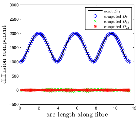
To compare the tangent and normal components quantitatively, we apply step 6 of Algorithm 1, computing the weighted averages over the fibre. The resulting averages for the drift are $\mu^{\text{tan}}_{\operatorname{avg}}=704.27$ and $\mu^{\text{nor}}_{\operatorname{avg}}=25.165$ and for the diffusion are $D^{\text{tan}}_{\operatorname{avg}}=1.4809\times 10^{3}$ and $D^{\text{nor}}=1.4216$. Note that $\mu^{\text{tan}}_{\operatorname{avg}}$ and $D^{\text{tan}}_{\operatorname{avg}}$ are both significant larger than $\mu^{\text{nor}}_{\operatorname{avg}}$ and $D^{\text{nor}}_{\operatorname{avg}}$. By step 7, we conclude that the system has multiscale behaviour.

We now apply Algorithms 2A and 2B to the system. Before discussing the numerics, first note that from the original equations (12) and (13), one sees that the dynamics on a fast vertical fibre in these original coordinates is given by an Ornstein–Uhlenbeck process with drift $(-y+\sin x)/\epsilon$ and diffusion ${1}/{\sqrt{\epsilon}}.$ For such processes, the eigenvalues of the Fokker–Planck operator can been determined analytically [19]. For (13), the eigenvalues are given exactly by $\lambda_{k}=-k/\epsilon$ for integers $k\geq 0$. Since the spectrum of the operator is not affected by a change of coordinates, these are also the exact values for the eigenvalues of the operator ${\widehat{\mathcal{L}}}_{\text{tan}}$ associated to the fast dynamics of the system given by (14)–(15).

In the application of Algorithm 1 above, we computed the values $\hat{\mu}_{1}$ and $\hat{D}_{11}$ at points uniformly distributed along the fast fibre $F$. These define a drift diffusion process along $F$ with associated Fokker–Planck operator ${\widehat{\mathcal{L}}}_{\text{tan}}$. Applying Algorithm 2B, we calculate leading eigenvalues $\widehat{\lambda}_{k}$ of this operator ${\widehat{\mathcal{L}}}_{\text{tan}}$ numerically. A fourth-order central finite difference method was used. The computed eigenvalues are given in the second column of Table 1. Note that the eigenvalues $\widehat{\lambda}_{k}$ are all of order $10^{3}$ and the eigenvalues $\lambda_{k}$ are of order $1$. Applying the final step of Algorithm 2B, the ratios $\operatorname{Re}(\lambda_{k})/\operatorname{Re}(\widehat{\lambda}_{k})$ are all between $10^{-4}$ and $10^{-3}$ and give an estimate of the time-scale separation. This agrees with the value $\epsilon=10^{-3}$ used in defining the system.

For each computed eigenvalue $\widehat{\lambda}_{k}$, the relative error

is also given in the table.

We now consider Algorithm 2A and perform eigenvalue calculations by expressing the fibre globally as a graph. A fast fibre $F$ is of the form $\{(x,y):x=\sin(y)+c\}$ for some constant $c$. Therefore, if $A$ is a rotation matrix

with $\theta$ between $45$ degrees and $135$ degrees, then $A(F)$ is the graph of a function $g:\mathbb{R}\to\mathbb{R}$. For values of $\theta$ at every $5$ degrees between $55$ and $125$, we applied Algorithm 2A with the corresponding $A$ and computed seven leading eigenvalues $\widehat{\lambda}^{(\theta)}_{0}>\widehat{\lambda}^{(\theta)}_{1}>\cdots>\widehat{\lambda}^{(\theta)}_{6}$ for the associated Fokker–Planck operator. This computation was achieved by first determining the values $\hat{\mu}_{1}(z_{n})$ and $\hat{D}_{11}(z_{n})$ for points $z_{n}:=(v_{n},g(v_{n}))\in A(F)$ where the $v_{n}$ are given by $200$ evenly spaced numbers across an interval in $\mathbb{R}$. Then, these sampled values of $\hat{\mu}_{1}$ and $\hat{D}_{11}$ are used to approximate the Fokker–Planck operator ${\widehat{\mathcal{L}}}_{\text{tan}}$ and the eigenvalues are solved using a fourth order central finite difference method. As noted above, the leading eigenvalues for the actual system are given by ${-k}/{\epsilon}$ and the computed values $\widehat{\lambda}^{(\theta)}_{k}$ agreed with these theoretical values with a relative error less than one percent for all computed $\theta$ and $1\leq k\leq 6$. This shows that Algorithm 2A produces estimates of the eigenvalues $\widehat{\lambda}_{k}^{(\theta)}$ for the fibre dynamics that are robust with respect to the parameterization the fibre.

Algorithms 1 and 2 have established the presence of multiscale behaviour for the system and determined the time-scale separation. As a final step, we compute the drift and diffusion data for the reduced slow system using the technique described in Section 6. We restrict the leading eigenfunctions $\psi_{1}$ and $\psi_{2}$ of the full system to the line $C=[0,2\pi]\times\{0\}$ which is transverse to the fast fibres. Each eigenfunction $\psi_{k}$ on the full space was solved numerically by collocation and the result is represented by the values that $\psi_{k}$ takes on a $50\times 50$ grid on $[0,2\pi]\times[-L,L]$. Restriction of this eigenfunction to $C$ may therefore be performed simply by taking the appropriate row from the matrix representing the computed function. The restriction $\psi_{k}|_{C}$ is then given by the values that the function takes on a set $X\times\{0\}$ consisting of $50$ points uniformly spaced along $C$. At each point $x\in X$, we look at a window of points consisting of $x$ and the ten other points in $X$ closest to $x$. Using these eleven data points, we fit a cubic polynomial to $\psi_{k}|_{C}$. This polynomial is used to estimate the first and second derivatives of $\tilde{\psi}_{k}\approx\psi_{k}|_{C}$ at the point $x$ which are then used to solve pointwise the linear equations given by (11).

References

- [1] Viviane Baladi. Correlation spectrum of quenched and annealed equilibrium states for random expanding maps. Comm. Math. Phys., 186(3):671–700, 1997.
- [2] John P. Boyd. Chebyshev and Fourier spectral methods. Dover Publications Inc., Mineola, NY, second edition, 2001.
- [3] D. Crommelin and E. Vanden-Eijnden. Diffusion estimation from multiscale data by operator eigenpairs. Multiscale Modeling & Simulation, 9(4):1588–1623, 2011.
- [4] D. T. Crommelin and E. Vanden-Eijnden. Reconstruction of diffusions using spectral data from timeseries. Communications in Mathematical Sciences, 4:651 – 668, 2006.
- [5] Michael Dellnitz and Oliver Junge. On the approximation of complicated dynamical behavior. SIAM J. Numer. Anal., 36(2):491–515, 1999.
- [6] Weinan E. Principles of Multiscale Modeling. Cambridge University Press, 2011.
- [7] Gary Froyland, Cecilia González-Tokman, and Anthony Quas. Detecting isolated spectrum of transfer and Koopman operators with Fourier analytic tools. Journal of Computational Dynamics, 1(2):249–278, 2014.
- [8] Gary Froyland, Georg A Gottwald, and Andy Hammerlindl. A computational method to extract macroscopic variables and their dynamics in multiscale systems. SIAM J. Appl. Dyn. Syst., 13(4):1816–1846, 2014.
- [9] Gary Froyland, Oliver Junge, and Péter Koltai. Estimating long-term behavior of flows without trajectory integration: the infinitesimal generator approach. SIAM J. Numer. Anal., 51(1):223–247, 2013.
- [10] Gary Froyland, Simon Lloyd, and Naratip Santitissadeekorn. Coherent sets for nonautonomous dynamical systems. Phys. D, 239(16):1527–1541, 2010.
- [11] Dror Givon, Raz Kupferman, and Andrew Stuart. Extracting macroscopic dynamics: model problems and algorithms. Nonlinearity, 17(6):R55–R127, 2004.
- [12] Emmanuel Gobet, Marc Hoffmann, and Markus Reiß. Nonparametric estimation of scalar diffusions based on low frequency data. Ann. Statist., 32(5):2223–2253, 2004.
- [13] E. Hairer, S. P. Nørsett, and G. Wanner. Solving ordinary differential equations. I, volume 8 of Springer Series in Computational Mathematics. Springer-Verlag, Berlin, second edition, 1993. Nonstiff problems.
- [14] Lars Peter Hansen, José Alexandre Scheinkman, and Nizar Touzi. Spectral methods for identifying scalar diffusions. J. Econometrics, 86(1):1–32, 1998.
- [15] Bernard Helffer and Francis Nier. Hypoelliptic estimates and spectral theory for Fokker-Planck operators and Witten Laplacians, volume 1862 of Lecture Notes in Mathematics. Springer-Verlag, Berlin, 2005.
- [16] Peter Henrici. Discrete variable methods in ordinary differential equations. John Wiley & Sons, Inc., New York-London, 1962.
- [17] Bernt Øksendal. Stochastic differential equations. Universitext. Springer-Verlag, Berlin, 1985. An introduction with applications.
- [18] G. A. Pavliotis and A. M. Stuart. Parameter estimation for multiscale diffusions. J. Stat. Phys., 127(4):741–781, 2007.
- [19] Peter Sjögren. Operators associated with the Hermite semigroup—a survey. In Proceedings of the conference dedicated to Professor Miguel de Guzmán (El Escorial, 1996), volume 3, pages 813–823, 1997.