Multi-scale metastable dynamics and the asymptotic stationary distribution of perturbed Markov chains
Abstract.
We consider a simple but important class of metastable discrete time Markov chains, which we call perturbed Markov chains. Basically, we assume that the transition matrices depend on a parameter , and converge as . We further assume that the chain is irreducible for but may have several essential communicating classes when . This leads to metastable behavior, possibly on multiple time scales. For each of the relevant time scales, we derive two effective chains. The first one describes the (possibly irreversible) metastable dynamics, while the second one is reversible and describes metastable escape probabilities. Closed probabilistic expressions are given for the asymptotic transition probabilities of these chains, but we also show how to compute them in a fast and numerically stable way. As a consequence, we obtain efficient algorithms for computing the committor function and the limiting stationary distribution.
Keywords: escape times, non-reversible Markov chains, asymptotics
2000 Math. Subj. Class.: 60J10, 60J22
1. Introduction
In this paper we give a detailed analysis of the asymptotic dynamics and stationary distribution for a special class of metastable Markov chains. Loosely speaking, a metastable Markov chain is one that, on short time scales, looks like a stationary Markov chain exploring only a small subset of its state space; on longer time scales, however, it performs fast and rare transitions between different such subsets.
The topic of metastability is an old one. Its origins can be traced back at least to the works of Eyring [10] and Kramers [13], who studied it in the context of chemical reaction rates. In the context of perturbed dynamical systems, Freidlin and Wentzell [11] developed a systematic approach based on large deviation theory. This approach was extended by Berglund and Gentz [3] to cover stochastic bifurcation and stochastic resonance, and by Olivieri and Scoppola [20, 21] to study dynamics of Markov chains with exponentially small transition probabilities. Bovier, Eckhoff, Gayrard and Klein [5, 6, 7] developed a systematic approach based on capacities, and gave a precise mathematical definition for metastability. The transition path theory [25, 26] investigates the most probable paths that the Markov chain uses when travelling between different metastable states. Recent books on various aspects of metastability include the monograph [19], and the lecture notes [4].
As we will discuss in Section 4, the chains treated in the present paper are metastable in the sense of Bovier et al. Our situation is considerably simpler than the general one: the state space is of fixed finite (but possibly large) size, and the metastability enters via an explicit parameter in the transition matrix. In contrast, the theory described in [5, 6, 7] is built to accommodate the difficult situation where metastability is not necessarily a consequence of some transition probabilities becoming small, but may also arise from a limit where the number of states diverges. In the case of reversible Markov chains, many of our main results can be deduced from the theory of [5, 6, 7], although our proofs are different and do not rely on the variational methods used there. The benefit of this is that our methods also cover the non-reversible situation where Dirichlet-form techniques are less useful.
Let us describe our setup and results in some more detail. Consider a family of discrete time Markov chains with finite state space and transition matrices . We assume that the map is continuous at for all , and that the Markov chain is irreducible when . For however, the chain may have several essential communicating classes. Such a family of Markov chains is called an irreducible perturbation of , or simply an irreducibly perturbed Markov chain.
The first main result of the paper is a description of the multi-scale metastable behavior of the chain. Let be the essential classes of the chain at parameter . We pick for all and define an effective chain with state space . We prove that this chain captures the effective dynamics of the original chain on the shortest metastable time scale, in the sense that its escape probabilities and stationary distribution are asymptotically independent of the choice of the representatives , and asymptotically equal to those of the original chain. For the stationary distribution, this means that , where and are the stationary distributions of the respective chains. A central tool is a natural, reversible chain that has the same stationary distribution as and is interesting in its own right.
In order to explore longer metastable time scales, we renormalize the effective chain: for , all transitions between different states will vanish in the limit . By rescaling time under suitable conditions, we obtain a new perturbed Markov chain, where at least one transition probability between distinct states is of order one as . We can now iterate the procedure described above, yielding effective chains on smaller and smaller state spaces and encoding the dynamics of the original chain on longer and longer metastable time scales.
A similar program has been carried out before by Olivieri and Scoppola [20, 21]. The difference to our approach is that [20, 21] relies on (and extends) the theory of Freidlin and Wentzell, while our approach is closer to the potential theoretic methods of Bovier et. al. [4]. This allows us to avoid many of the technical complications found in [20, 21]. Also, Olivieri and Scoppola only consider Markov chains with exponentially small transition probabilities, and study asymptotics on a logarithmic scale. In contrast, our methods allow for much more general families of transition matrices, and our results are asymptotically sharp in the sense that we identify the correct prefactors for all our asymptotic identities. The last fact is particularly useful in practice, since it allows us to devise numerically stable algorithms for computing the asymptotic stationary distribution for all states . Alternatively, we can compute the ratio of the stationary distributions for two given states without computing the full stationary distribution, thus potentially decreasing the computational cost considerably. These algorithms are the second main result of our work.
To see why numerically computing the asymptotic stationary distribution might be a problem, consider the following simple example. Let , and with elements , , for some . For , and are the essential classes of the chain, so both and are metastable. The stationary distribution of the chain is , . Thus depends very sensitively on the behavior of the elements of the transition matrix at small .
The reason for this is that the space of solutions to the defining equation is one-dimensional in the case , but multidimensional in the case . This also means that this linear equation is ill-conditioned for small . Thus computing numerically by solving an eigenvalue problem is infeasible if the state space is large and the transition matrix is somewhat complicated. Metastability also means that a Monte Carlo simulation of , i.e. running the chain and recording the relative occupation times of the states , will fail for small . In the reversible case, the detailed balance equation can be used to compare the relative importance of and for neighboring , and by iterating for all , but there is no detailed balance equation for irreversible Markov chains. Therefore, it is not immediately clear how to compute the asymptotic stationary distribution of an irreversible perturbed Markov chain in any numerically efficient way.
Efficiently computing the stationary distribution of a large Markov chain is an extremely important problem in many areas of applied science. Maybe the most prominent example where it is needed is the computation of the page rank in search engines [14], where metastability also plays a role. It is therefore not surprising that a large body of literature is devoted to the topic, mainly in the computer science community. The seminal paper here seems to be by Simon and Ando [22], where they introduce a method for treating what is now known as almost decomposable Markov chains, and derive the metastable behavior and some information on the asymptotic stationary measure for such chains. Subsequently, the method was clarified and extended, and Meyer [17] realized that many of the extensions have a common foundation that he called the theory of the stochastic complement. Many further extensions and refinements of the method have been given since. We cannot give a full review of the literature here, but rather point the reader, by way of example, to the recent papers [24, 18, 23] and the references therein.
An apparently independent effort to treat metastable Markov chains took place in the context of game theory and mathematical economy. Here the start was made by HP Young [29]. He basically advocated using the Markov chain tree theorem, as given in [1] or [11]. Up to normalization, it gives the stationary measure as the sum of terms indexed by the directed spanning trees of rooted in , where the weight of a tree is the product of all transition probabilities along its edges; for details see [1]. As has been pointed out in [9], the problem with this formula is that while it is in principle not numerically unstable, it involves computing all spanning trees, which is exponentially expensive and thus becomes non tractable for large state spaces. Moreover, all of the are usually tiny, and so we are trying to add an astronomical number of tiny terms, which is not a good idea.
A different approach was taken by Wicks and Greenwald [27, 28] who offer a solution that is closer to the one described in [17], but differs in some important details. At the center of their method is what they call the quotient construction on stochastic matrices, which allows them to recursively simplify the state space and, by keeping track of the various simplifications, to compute in the end.
As can already be guessed from the above discussion, the citation graph on metastable Markov chains and their stationary distributions is somewhat disconnected. While some mathematicians, e.g. [15] or [8], are aware of the theory of Ando and Simon [22], it does not seem to be well known in the probability theory community. On the other hand, the mathematical theory of metastability following [5] is virtually unknown in the applied community, and the approaches by Young [29] and Wicks and Greenwald [28] appear to be completely disjoint from the others. We hope that, among its other purposes, this paper helps connect these communities. For this reason we review the results related to Simon/Ando and those of Wicks/Greenwald at the end of our paper, translate their statements from the language of matrices to probabilistic terminology, and comment on how their results relate to the present paper.
The paper is organized as follows: in Section 2, we collect some results on escape times for irreducible Markov chains that seem hard to find in the literature. In Section 3, we introduce perturbed Markov chains and show how the results from Section 2 can be used to obtain asymptotic expressions of various important quantities. These will be used in Section 4 to describe the multi-scale effective dynamics of the chain. Finally, in Section 5, we present our numerical algorithms and compare them to those present in the computer science and economics literature.
2. Stationary measures, escape probabilities and hitting distributions
Here we collect the main tools that we will use. In this section, is a general discrete time Markov chain. In contrast to the remainder of the paper, we do not assume the state space to be finite, but we will assume that is irreducible and recurrent unless stated otherwise.
All of the results below are relatively transparent, explicit identities involving hitting times. Given the sheer amount of material on the subject, it is reasonable to assume that some or all of them have been derived elsewhere. We were unable to find an explicit reference for any of them, but will comment on related results where appropriate.
For a Markov chain on a state space , the hitting time of a set is denoted by , and the return time by . As usual, we will write instead of for , and similarly for .
Proposition 2.1.
Assume that is irreducible and positive recurrent, and write for the unique stationary distribution. Then for all ,
| (2.1) |
Proposition 2.1 looks like it should be part of every textbook on discrete time Markov chains, but somewhat surprisingly it is not. Before we comment on the status of Proposition 2.1 in the literature, note that (2.1) is reminiscent of the detailed balance equation. Let us write and for the moment assume that for all . Then the quantities can be completed to become the transition matrix of a reversible Markov chain that has the same stationary distribution as . In general, will not hold for all , but below we will encounter a situation in the context of perturbed Markov chains where it does.
When the Markov chain itself is reversible, Proposition 2.1 is a direct consequence of the well established theory of electrical networks: for example, from Proposition 9.5 in [16] it follows that , where is the effective conductance between and , and a global constant. Since is symmetric in and , (2.1) follows in the reversible case.
For the non-reversible case, Proposition 2.1 appears much less well known, although it can also be quickly deduced from a known result: Corollary 8 of Chapter 2 in the unfinished, but brilliant, monograph by Aldous and Fill [1] directly implies it. As we have not found that statement anywhere else, we give a short proof here for the convenience of the reader. Our proof differs somewhat from the one given in [1] and uses the following more general lemma:
Lemma 2.2.
Let be irreducible and positive recurrent. For all states ,
Proof.
Since the chain is irreducible and positive recurrent, for all and in the state space , so in particular almost surely. Thus
The first two terms of the last line above sum up to . The last term is equal to , where denotes the time shift by steps. Indeed, the random variables and , when nonzero, both count the number of steps from the first occurrence of until the first occurrence of . By the strong Markov property,
and the claim follows. ∎
Proof of Proposition 2.1.
If , the claim boils down to , so let us assume that . By using Lemma 2.2 in two different ways we obtain
| (2.2) |
We rearrange the second equation above to obtain
the last equality being due to . Plugging this back into the first line of (2.2), using the fact that , and rearranging, gives
| (2.3) |
which is essentially Corollary 8 of Chapter 2 of [1]. For our purposes, we note that the right-hand side of (2.3) is invariant under swapping and , which proves the claim. ∎
Remark: In the continuous time setting, the whole proof of Lemma 2.2 and almost all of the proof of Proposition 2.1 goes through unchanged if we define The only difference is that the formula for the stationary measure in that case is given by , where is the exponential rate with which the process jumps away from . This gives the formula
which is a special case of the symmetry result on capacities for non-reversible continuous time Markov chains derived by Gaudilliére and Landim [12], and applied to investigate metastability by Beltrán and Landim [2]. Their proof is quite different from the one presented here.
A direct consequence of Proposition 2.1 is
Corollary 2.3.
The stationary distribution of fulfills the set of equations
| (2.4) |
Proof.
Since if , (2.1) is equivalent to
for all . We have by irreducibility for all , and so we can divide both sides by it. Summing over and rearranging now shows the claim. ∎
To get the most out of Corollary 2.3, we need find a way to compute the escape probabilities appearing in (2.4). We will now collect some tools that will help us to do this, asymptotically, in the context of perturbed Markov chains. Unlike the statement of Proposition 2.1, we have not been able to find them in the literature, but we still suspect that they are not completely new.
Proposition 2.4.
Let be an irreducible, recurrent Markov chain. For , and , we have
| (2.5) |
When , (2.5) simplifies to
| (2.6) |
Proof.
For , let us write for the set of paths that visit precisely times before entering , and in addition move directly from to . More formally, we put , and
for , where denotes the cardinality of a set in this case. Then,
We have , and the sets are disjoint. As the chain is irreducible and recurrent, holds, and thus
| (2.7) |
Now for we compute
In the second line, we used the strong Markov property, and in the third line, finite induction. We now sum up the geometric series in , use , and obtain
In the last equality we used that implies . Plugging this into (2.7) proves (2.5).
A variant of Proposition 2.4 is well known and is the basis of many algorithms for computing stationary distributions of large Markov chains. It is called the quotient construction by Wicks and Greenwald [27, 28], and the stochastic complement by Meyer [17]. While in all those references, it is written in matrix language, we give here the probabilistic formulation, which also has the benefit that we can give a short and transparent proof. Below and in what follows denotes the complement of a set .
Proposition 2.5.
Proof.
Clearly, . Now, standard results [16] state that is the unique harmonic extension of the function from to . In other words, is the unique function so that for all , and on . This can be rewritten as for all . Since is irreducible, there exists with , where is the operator norm of a matrix. Thus is invertible. The claim follows. ∎
Remark: In (2.8), the probability of the set of all paths moving from to in and then entering from there is expressed as . In (2.5) the probability of the set of all paths that leave at but enter anywhere is expressed as the quotient of two escape probabilities. Comparing the two and varying over leads to the amusing identity
for all , and .
For the following result, we do not assume irreducibility of the chain.
Lemma 2.6.
Let be an arbitrary Markov chain, . Assume and . Then
Proof.
We have
where in the last step we have used the strong Markov property. By our assumption , we have . Since we assumed , we must have ; otherwise the strong Markov property would give . Thus we can rearrange and obtain the result. ∎
For our next statement, fix a proper subset , and define for all
| (2.9) |
Proposition 2.7.
Let be an irreducible, recurrent Markov chain. Then is the transition matrix of a Markov chain . Denoting its path measure by , we have
| (2.10) |
for all with , and all .
Proof.
Since is irreducible and recurrent and , for all . Thus it is obvious that is a stochastic matrix. The statement (2.10) is also intuitively obvious, since all we do is replace the motion inside with the effective motion from to its exterior. We nevertheless give the short formal proof.
We write for the -th time that the chain travels between two states that are not both in , i.e.
On , we define . Then for all by recurrence and irreducibility of , and is a Markov chain by the strong Markov property of . Since , the transition probabilities of are given by (2.9). Since is disjoint from and , we have
and (2.10) follows by taking expectations. ∎
For our final general statement, we introduce the notion of a direct path which will be useful in several places below. Let , and be subsets of . A tuple is called a direct -path of length from to if , , and for all , if then and . Note that we allow . The set of all direct -paths from to will be denoted by , and the components of will be written , . will denote the length of . For or we will use the notations instead of etc, and speak of direct -paths from to , from to or from to . The probability of a direct -path is defined by .
Proposition 2.8.
Let be a finite subset of . Then for all and ,
| (2.11) |
Proof.
The idea of the proof is to start at state and run the Markov chain until it either hits or returns to . In the first case we have reduced the problem to computing and we iterate the argument for the smaller set ; in the second case we use the strong Markov property to restart the process. Formally, let us proceed by induction on . The claim trivially holds for ; so now let . The third equality below is obtained by the strong Markov property.
As the Markov chain is recurrent and irreducible, we have . Thus the last equation can be rearranged to
where the numerator may be decomposed as .
Finally, we use the induction hypothesis for the set to rewrite for all , and obtain
Re-indexing yields the claim. ∎
3. Perturbed Markov chains: escape probabilities
Let be a Markov chain on a finite state space . A family of Markov chains on indexed by is called a perturbation of if for all , where denotes the elements of the transition matrix of the chain , . We will speak of an irreducible perturbation of (or, alternatively, call the family an irreducibly perturbed Markov chain) if the chain is irreducible for all .
Note that in the definition of irreducibly perturbed Markov chains, we do not require that be irreducible, and indeed the case where has several ergodic components is the interesting one. Recall that is called accessible from under if for some . We write if is accessible from , and say that two states and communicate if and . The property to communicate forms an equivalence relation, and the respective equivalence classes are called communicating classes. A state is called essential if for all such that , otherwise transient. It is easy to see that either all members of a communicating class are essential, or all are transient. In the first case, is called an essential (communicating) class, or ergodic component.
can thus be decomposed into finitely many disjoint essential classes and the set of transient states. To emphasize that a nontrivial ergodic decomposition only exists for , we will always speak of -essential classes and -transient states. will denote the set of all -essential classes.
The sets and can be conveniently described in terms direct paths. The following statement could be taken as a definition of -essential classes and -transient states; the proof of equivalence to the traditional definition of essential classes (see e.g. [16]) is very easy, and omitted here. Here and below, we will say that a direct path is -relevant if , otherwise -irrelevant.
Lemma 3.1.
Let be an irreducibly perturbed Markov chain.
a) are in the same -essential class if and only if there exists
a -relevant direct -path from to , and a -relevant
direct -path from to .
b) is in the transient set if and only if all
direct -paths from to are -irrelevant.
In much of what follows, we will use the following concept of asymptotic equivalence. Two functions and from to are asymptotically equivalent, if either and are identically zero, or for all with some and . Note that in the latter case, we do not assume convergence of or . We write if is asymptotically equivalent to . It is easy to see that is indeed an equivalence relation, and in particular this implies whenever and is not identically zero. We will also need to know that is stable under addition and multiplication in the following sense: if and , then , and . Stability under multiplication is trivial, and stability under addition follows from
and transitivity of . Note that we did not assume that in either case.
Let be a -essential class. The restriction of to is the Markov chain with state space and transition matrix . It is irreducible, and thus has a unique strictly positive stationary distribution . The trivial extension of to (by putting for ) will be denoted by the same symbol, and is an extremal point of the convex set of stationary distributions for . The following lemma shows that when we focus our attention on a single -essential class, the unperturbed chain gives a faithful asymptotic description of both the dynamics and the stationary distribution. Here and below we will write for the unique stationary distribution of , when .
Lemma 3.2.
Let be a -essential class. Then for all and all ,
| (3.1) |
and
| (3.2) |
In particular, .
Proof.
We only prove the first equality from (3.1), the proof for the second one is identical. We decompose
| (3.3) |
The second term is equal to , and Proposition 2.4 gives
Now for each , there is a -relevant direct -path from to , and so
Thus , and thus the second term on the right-hand side of (3.3) vanishes as .
For the first term of (3.3), fix and decompose
We have
The first equality is because the probability on the left-hand side is a finite sum of at most -fold products of transition probabilities. The elementary Markov property at time gives
For each , there is a -relevant direct -path from to , and thus there exists with for all sufficiently small. We conclude that for all sufficiently small and thus
As was arbitrary, (3.1) follows. For (3.2), we apply (2.1) and obtain
Since the right-hand side above is strictly positive, this implies . ∎
As an immediate corollary, we obtain some information on the structure of the stationary distribution in the limit . Recall that is the collection of -essential classes, and is the set of transient states.
Corollary 3.3.
Let .
a) If , then .
b) If for some , then
.
c) In particular if exists for all , then
exists for all , and
Proof.
The practical usefulness of Corollary 3.3 depends on our ability to compute asymptotic expressions for the . We now give two statements that will play a key role in all that follows. The first says that hitting probabilities are asymptotically equivalent when the transition matrices are. The second describes how a perturbed Markov chain leaves a -essential class, with or without the additional condition that it cannot return to its starting point.
Theorem 3.4.
Let and be perturbed Markov chains with finite state space , but not necessarily irreducible. Let us assume that for the elements of the respective transition matrices. Then for all and all , we have
Proof.
We will first show that the statement holds in the case where and only differ in one row, i.e. where
| (3.4) |
Once this is done, we can exploit the assumption that is finite, iteratively change row after row, and prove the full claim. For the case where (3.4) holds, first note that for all ,
This can be seen by considering a coupling of the chains and by observing that by (3.4), for all . So, the first time when the chains and can differ is after they hit . Thus,
Since , we can now use the strong Markov property to find
Again , and it remains to show that . If , this is trivial. For , , and . We are aiming to use Lemma 2.6, and thus need to deal with the possibility that .
We assumed for all , and so we also have for each direct path from to . By the definition of , a direct path from to fulfills for all in a neighborhood of if and only if in a neighborhood of . Let us first assume that no such direct path exists. Then for all , and thus . Now let us assume that such direct paths do exist. Since , we can use Lemma 2.6 to get
Now,
and the same argument shows . The claim follows. ∎
The statement of Theorem 3.4 is rather surprising. The reason is that even though in each step that the chain takes from on its way to , the probabilities for the chains and differ only by a factor that becomes negligibly close to one as , in the same limit the number of steps needed to reach can diverge. Indeed, imagine two -essential classes and that are linked by direct paths with , but are linked to and only by paths with . Then, starting from a point in , both and will be visited many times before either or is hit. So one could fear that the errors committed by changing each transition probability to an asymptotically equivalent one will pile up; but as Theorem 3.4 shows, this is not the case.
Theorem 3.5.
Let be a -essential class, and . Then
| (3.5) |
and
| (3.6) |
with normalizing constant
Remark: (3.6) is intuitively clear: for small , the Markov chain spends such a long time in before exiting that it essentially exits from its -stationary distribution. Formula (3.5) on the other hand is rather remarkable, since a return to happens in a time of order one, so there is no time for the chain to become stationary.
Proof of Theorem 3.5.
To prove (3.5), choose in Proposition 2.4. Then
We decompose
| (3.7) |
The first term is equal to . The second term in this decomposition as well as the second term in (3.7) are bounded by and thus vanish , due to Lemma 3.2 and the finiteness of . The same Lemma then yields
Similarly, for we have
By Proposition 2.1, we conclude
Here, we have used that for all . Since the right-hand side above is strictly positive, we conclude that , and (3.5) is shown.
4. Perturbed Markov chains: metastable dynamics
Here we describe the metastable dynamics of a perturbed Markov chain. As in the previous section, we will restrict our attention to a finite state space throughout.
First of all, we have to define what we mean by metastable dynamics. We follow the theory of Bovier et al [5, 6, 7]. In the case of perturbed Markov chains on a finite state space, Definition 2.1 from [5] (see also [4]) goes as follows: a set is called a set of metastable points if for all and ,
| (4.1) |
In words, this means that reaching from the outside of is much easier than traveling between different points of , in both cases with the restriction not to return to one’s starting point first.
Using Lemma 3.1 and Lemma 3.2, it is easy to see that if we choose precisely one point from each of the -essential classes , then the set is a set of metastable points. Also, is maximal in the sense that adding a further point to will result in a set no longer fulfilling (4.1). On the other hand, removing points from or replacing them with points from may in certain cases still result in a metastable set, depending on the structure of the Markov chain and the points in question. We will not pursue this further since is the most natural choice. Of course, when some of the contain more than one point, the choice of is not unique. One of our main results is that when defining the effective chain by the transition matrix
| (4.2) |
then the relevant dynamical quantities will be asymptotically independent of the choice of the representatives .
The occurrence of the expression in (4.2) is intuitively obvious, since it means that we just monitor the chain when it hits one of our reference points . The factor may be less obvious. To motivate it, note that by (3.5),
| (4.3) |
This shows that the factor in (4.2) cancels one of the dependencies of on the choice of our set . While the terms still do depend on the choice of , we will see below that including the factor in the definition is enough to obtain the asymptotically correct stationary distribution and escape probabilities. This justifies the following definition:
Definition 1.
Let be an irreducibly perturbed Markov chain on a finite state space. The Markov chain with state space and transition matrix (4.2) is called the effective metastable representation of corresponding to .
In order to show the properties of the chain announced above, we define a second effective Markov chain, this time without reference to a set of representatives. For with we put
| (4.4) |
and . The are the elements of a transition matrix when is sufficiently small. As the following Proposition shows, this chain is reversible and the reversible measure of is :
Proposition 4.1.
The quantities satisfy the asymptotic detailed balance equation
The proof of Proposition 4.1 rests on the following simple lemma:
Lemma 4.2.
Let be -essential classes, , , , and . Then
| (4.5) |
Proof.
Proof of Proposition 4.1.
When , the claim holds trivially. For , pick and . We use Corollary 3.3 b), Proposition 2.1, and Corollary 3.3 b) again to find
Thus by (4.5),
| (4.6) |
for all . Since the right-hand side is independent of , and the left-hand side is independent of , we find
| (4.7) |
for all , and similarly for . Thus when we multiply (4.6) with and sum over and , we obtain the claim. ∎
The next result shows that the effective metastable representation indeed describes the metastable dynamics of correctly, in the sense that asymptotically it has the right escape probabilities and thus the right stationary distribution. Let us write for the stationary distribution and for the path measure of .
Theorem 4.3.
For , we have . In particular .
Proof.
From (4.7) and Lemma 4.2, we see that
The Markov property and the definition of then gives
We will show below that for ,
| (4.8) |
Once this is done, the Markov property for shows the first claim, and from Proposition 4.1 we get
Since by Proposition 2.1, we get
Since by Corollary 3.3 a), we can sum over and obtain , and thus .
To show (4.8), we introduce the shorthand
From (4.2), we get . Now a standard application of the Markov property with the stopping time shows that for , is the unique solution of the harmonic equation for all with boundary conditions , . Likewise, is the unique solution of the harmonic equation for all with boundary conditions , . But since
we must have , and the claim follows. ∎
The advantage of the chain is that its transition matrix is almost diagonal in the sense that . In particular, is an irreducible perturbation of the trivial (identity) Markov chain. It is now natural to rescale time so that the most likely transition between two different states becomes of order one. More precisely, we set
| (4.9) |
Since , for each at least one of the terms in the finite sum must be large. The problem is that at this point we cannot guarantee that the quantities converge. To see what could happen, consider the example , , . Then , but does not converge. Of course, this also implies that does not exist.
So far, we did not have to pay attention to that type of problem - all of our results above are valid as asymptotic equivalences, whether or not the quantities in question converge. Now however, we need proper convergence to carry on, and will give a sufficient criterion. Let , be two functions of . We say that and are asymptotically comparable, and write , if either both of them are strictly positive and exists in , or if one or both of them are identically zero. Note that we allow and as possible limits. We caution the reader that unlike asymptotic equivalence, asymptotic comparability is not transitive, and is not stable under multiplications. On the other hand, it is obviously symmetric, and we have the following summability property: If , and are mutually asymptotically comparable, and if and have strictly positive, finite limits as , then
| (4.10) |
We say that an irreducibly perturbed Markov chain is regular if for all and all sequences of pairs , with , we have
| (4.11) |
We will call a transition matrix regular if the generated Markov chain is regular.
Examples of regular perturbed Markov chains include those treated in [28], where the transition elements are of the form with either converging to a strictly positive limit or identically zero, and independent of . They also include those with property introduced in [21].
Theorem 4.4.
Proof.
By (4.3), for
| (4.12) |
and Proposition 2.8 gives
| (4.13) |
In Lemma 4.5 below we will show that if contains one representative of each -essential class then exists and is strictly smaller than one for all . Thus each exists. In other words, is given as a sum of terms of the form with , where exists for all . When plugging this into (4.12), we can apply the extension of (4.10) to finite sums to show that is the transition matrix of a regular Markov chain. By (4.9), this immediately implies convergence of the transition probabilities . Rewriting the second equation in (4.9) in the form
we see in addition that the chain is a regular perturbed Markov chain. ∎
It remains to prove the claim used in the proof above.
Lemma 4.5.
Let be a perturbed Markov chain. Assume that a set contains one element of each -essential class. Let with . Then for all , exists and is strictly smaller than .
Proof.
As contains a representative of each -essential class, there must be a -relevant direct path from to some . So, .
For the existence of the limit, let first . For , we have as . Let us now assume that the claim holds for all such that with some . Let be such that . Then,
By the induction hypothesis, exists and is strictly smaller than . Thus also exists and is strictly smaller than . The claim follows by induction. ∎
We have thus found a way to successively describe the multi-scale metastable dynamics of regular perturbed Markov chains: starting with the original chain , we derive and then . By Theorem 4.4, and are again regular perturbed Markov chains. Moreover, all of the -essential classes consist of exactly one element, and whenever . So, describes the effective metastable dynamics, but still in the original time scale.
The transformation from to means that we go to a time scale where the most likely transitions between different states become of order one. In other words, there exist with . By Lemma 3.1, this implies that will no longer be a -essential class on its own: it will either form a larger -essential class together with some , , or it will have become -transient. In any case, the number of -essential classes will be smaller than the number of -essential classes. Thus by applying the transformations to the matrix , and iterating the procedure, we can recursively explore longer and longer time scales of the dynamics.
On a purely theoretical level, our theory of multi-scale metastable dynamics for regular perturbed Markov chains is thus complete. However, if one attempts to (numerically) compute the transition probabilities at the different time scales, the problem arises that all relevant expressions in our theory still contain terms of the form . In the next section, we will show why naive attempts to compute this quantity numerically are likely to fail, and present a numerically stable algorithm for computing them. A byproduct of our algorithm is a numerically stable method to compute the matrix elements of the transition matrix , and thus the stationary weights for all -essential classes .
5. Computing hitting probabilities and the asymptotic stationary distribution
This section deals with aspects of the numerical computation of the transition probabilities and given in (4.2) and (4.4), respectively. Before we proceed we would like to make clear that subtle issues coming from the field of computable analysis fall beyond the scope of this article. Intuitively though, we mean the following by ”numerical computation”: if someone enumerates, step by step, all members of an infinite sequence of transition matrices that converge towards , we are able to process each using only a computer and produce, step by step, an infinite sequence that converges towards the matrices (or ). This corresponds roughly to the property of being computably approximable. Note that in this case we do not know how fast the sequence is converging to the limit. Said otherwise, if we want a precise approximation of, say, , we have no idea until which we should process the . This is a usual issue in numerical analysis. If in addition we would know that the -th approximation is, e.g., at most away from the limit, we would know when to stop to obtain the desired precision. This corresponds roughly to the property of being computable.
The starting point of our considerations are the formulae
| (5.1) |
and
| (5.2) |
both of which are obtained from the definition of the respective quantities using the strong Markov property. In both cases, the task is to compute a hitting probability of the form
| (5.3) |
where and . In the case of , and . Such hitting probabilities are well understood in the theory of Markov processes: is called the committor function in [25, 26] and the equilibrium potential of the capacitator in [4], and is the unique harmonic continuation from to of the indicator function of . This means that is the unique solution of the linear system
| (5.4) |
where . Let us write for the restriction of to . If and is irreducible, we have seen in the proof of Proposition 2.5 that is invertible. We thus find the committor function by matrix inversion:
| (5.5) |
The problem with this formula is that as , the matrix may converge to a non-invertible matrix. In that case, some matrix elements of will diverge, and even though the quantities themselves are bounded by for all , computing them numerically becomes unreliable as . Our first result will identify situations where this cannot happen.
We call a state an asymptotic dynamical trap (or simply a trap) with respect to if
A necessary condition for to be a trap is that there exists no direct -relevant path from into . On the other hand, for all there is at least one -relevant path from to some -essential class. Thus if intersects all -essential classes, no traps will exist.
Recall that for a matrix , the condition number is given by , where is the operator norm with respect to any norm on the underlying vector space. In our case, it is convenient to use the supremum norm on the vector space.
Proposition 5.1.
Assume that is such that there are no asymptotic dynamical traps with respect to . Then .
Proof.
Since is substochastic, clearly . On the other hand, the absence of traps with respect to allows us to find and , both of them independent of , and so that for all . The strong Markov property then implies for all and all . Thus for and bounded , we find
Consequently, the left-hand side above is absolutely summable, and
for all . Taking the supremum over , the claim follows. ∎
By construction, contains precisely one point of each -essential class, and thus there are no asymptotic dynamical traps with respect to . By Proposition 5.1 and (5.1) we can thus compute in a numerically stable way. In fact, the perturbative nature of the problem makes the following Newton scheme particularly useful.
Let denote the restriction of to , and set . By (5.5), we need to find . We use as a seed for the Newton iteration, and employ the usual recursion . By putting , we find and . So, is a polynomial in , and we can use the resulting commutativity to obtain
| (5.6) |
for all . In the special case , this can be transformed to
| (5.7) |
Thus
and
Proposition 5.1 guarantees that we can choose sufficiently small so that converges to very quickly. To illustrate this, we restrict ourselves to the special case where with the matrix bounded uniformly in . Then, for some , and
This means that when we are interested only in transitions of size or bigger, we only have to calculate logarithmically (in ) many . Therefore, it might seem that all is well, but this is not entirely so.
The reason is that a subtle problem arises from the multi-scale structure of the dynamics: at a given metastable time scale, it is in general not obvious what computational accuracy we need to achieve in order to obtain the asymptotically correct dynamics on longer metastable time scales. This phenomenon can best be explained by an example.
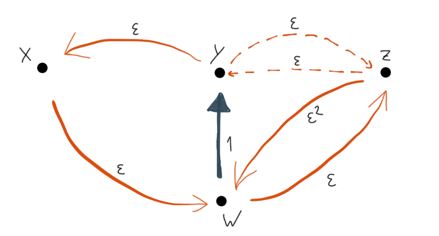
Figure 1 shows a graphical representation of a couple of metastable Markov chains. For both of them, , and both of them have transition probabilities corresponding to the solid arrows: , , and . Only one of them has the dashed arrows, i.e. . All other transition probabilities are zero except those mapping a point to itself, which are adjusted to give a stochastic matrix. With or without the dashed arrows, , and are the -essential classes, while is -transient. Also in both cases, , while . So on the first metastable time scale, transitions from to play no role. But whether or not we can stop our computation of after reaching order depends on the presence of the dashed arrows.
If the dashed arrows are present, we can stop the computation of after reaching order : on the next (and final) metastable time scale, we will have and . will be connected to via , by transition probabilities of order one.
However, if the dashed arrows are absent, stopping the calculation at order leads to an effective Markov chain where cannot be reached from , and thus to wrong results on the next metastable time scale. In the correct dynamics on that time scale and form a new effective metastable state, and transitions between it and are (after rescaling) of order . For this to be resolved correctly, the transition from to of order needs to be present already in the effective dynamics on the first metastable time scale.
In the simple example at hand it is easy to directly figure out what is going on, but to decide when a given approximation of is good enough to give correct dynamical results on all further metastable time scales for general chains on large state spaces is a subtle problem. Here we only give a necessary condition, about which we conjecture that it is also sufficient, and which is accessible to numerical validation. Let us write for path measure of a given approximation to the chain . By Theorem 4.3, when is the representative from and the representative from , and thus for all . So in order to obtain the correct asymptotic stationary distribution for our approximate chain, we have to increase the accuracy at least until
| (5.8) |
It would not be surprising if this were already sufficient for some sort of agreement of the metastable dynamics on all further metastable time scales. Since in general the escape probabilities do not characterize the transition probabilities of a Markov chain, a proof of this conjecture is not immediate, and we do not pursue this any further here. Instead, we discuss how to check (5.8) numerically.
By (5.2), the numerically tricky part in computing is . Since will not intersect all -essential classes unless there are only two of them, we cannot use Proposition 5.1 this time, and indeed in most situations a direct calculation of (5.5) will be numerically unreliable. However, for the very same reason, namely since intersects only two -essential classes, we can successively lift these traps and arrive at a simplified chain without traps for which the probability of hitting before is asymptotically equivalent to the original one.
The basic step in this procedure is the following. Assume that is a -essential class of a perturbed Markov chain , and that . We define a new Markov chain on the state space by its transition probabilities , where whenever , and
| (5.9) |
for all . Here, is the normalization that ensures that is a stochastic matrix. We say that the traps in (with respect to ) have been lifted in . This terminology is justified by
Theorem 5.2.
Let be a perturbed Markov chain, a -essential class
of , and the Markov chain where has been lifted.
a) Let .
Then for all , , while for ,
.
b) If is regular, then
is a regular perturbed Markov chain.
c) If is regular, then
either is a -transient state, or is an element of a
-essential class that
contains at least one further element . In the latter case, the number
of -transient states is strictly smaller than the number of
-transient states.
Proof.
Consider the chain with state space and transition matrix , where when and when . Denoting its path measure by , Proposition 2.7 gives for all . We now define by replacing with for , and keeping them the same if . Then (3.6) implies that for all , and thus Theorem 3.4 gives . Finally, noting that does not depend on whenever , we can replace all by a single state , and claim a) follows.
For b), note that by regularity of the chain, for all . So the quotient in (5.9) either converges or diverges to infinity as . Since it is bounded by by construction, the latter is not an option, and the converge. So the Markov chain defined by them is a perturbed Markov chain. Finally, this Markov chain is again regular, since products of its elements can be written as weighted sums of products of the with nonnegative weights. We have shown b).
For c), note that by b) exists, and since , there must be at least one state with . Lemma 3.1 implies that if is a -essential class with , then all direct paths from to are -irrelevant. So if one of the elements with is connected to a different -essential class via a -relevant direct path, then is -transient. On the other hand, if no is connected to any by such a direct path, then each such must be an element of , and must be connected to by a -relevant direct path. It follows that is in the same -essential class as , and thus not a -transient state. The claim follows. ∎
Using Theorem 5.2, we can now give a general recursive algorithm for numerically computing expressions of the form given in (5.3) simultaneously for all , up to asymptotic equivalence:
- (1)
Determine the set of all -essential classes not intersecting .
- (2)
If , compute by solving the well-conditioned linear system (5.4). Finish the algorithm.
- (3)
Compute the -stationary measures for each .
- (4)
Lift all the traps in by (5.9). This results in a new state space, where all elements of are replaced by a single state . Keep track of the elements of the original state space that become lumped into .
- (5)
Return to (1) with the new state space.
We note that steps (3) and (4) are trivial to parallelize. By Theorem 5.2 c), each step either decreases the number of -essential classes in the chain, or leaves it unchanged and decreases the number of transient states. We thus see that the algorithm terminates. Once it does (in step 2), we know for all in the final state space . Theorem 5.2 a) now guarantees that for all states of the chain from the previous step that were collapsed into . Thus we can recursively go backwards until we reach the original state space, where we now know all up to asymptotic equivalence. In particular, this gives a stable algorithm for the asymptotic numerical approximation of the coefficients . Since the expressions are also escape probabilities (for a different Markov chain), we can compute them by the same algorithm. If they agree with to leading order in , our necessary criterion is met and the approximate chain has the same asymptotic stationary measure as the true one.
Another useful aspect of our algorithm is that the determine the limiting stationary distribution of the chain through the formula
which is derived in analogy to (2.4), using Proposition 4.1. Computing the stationary distribution of a large Markov chain with many metastable sets is a very important problem in practice. For example, it is how internet search engines compute page importance ranks. As a consequence, there has been tremendous activity in the computer science community on the topic. Most of the developments seem to be based on a seminal paper by Simon and Ando [22]. Seemingly independently, the problem has been treated by a much smaller group of people in mathematical economy, starting with [29] and with significant recent progress by Wicks and Greenwald [27, 28].
Both approaches are based on formula (2.8), which itself is closely related to (5.4). In the literature following [22] and [17], this leads to what is known as the method of the stochastic complement. For a finite Markov chain on a state space , the first step of the method is to decompose into disjoint sets . Equation (2.8) with then allows to compute
| (5.10) |
for by using matrix multiplications and by computing the inverse of the matrix . The are the transition probabilities of an effective Markov chain only running inside . Writing for the stationary distribution of the effective chain, and for the full stationary distribution, it can be shown that
| (5.11) |
for all , where is the stationary distribution of the Markov chain with state space and transition probabilities
| (5.12) |
Equation (5.11) is similar to the statements of our Corollary 3.3, with the taking the role of , and the the role of . Equation (5.12) is in analogy to the expression
| (5.13) |
that we get for when combining (4.2) and (4.3). The drawback of the method is that a priori, we have no control over the numerical difficulty of computing . For example, let consist of two elements . Then , and thus the computation of is no easier than the problem we have treated in the present paper; in particular, if is a perturbed Markov chain and and are in different -essential classes, the matrix will become singular as . Therefore without any further assumptions, the theory of Simon and Ando as it stands gives no numerically feasible way of computing .
A suitable such further assumption is to choose the decomposition in a way that makes all transitions between different small. The situation where this is possible has been treated already in [22], and is nowadays known as a the theory of nearly reducible (or nearly decomposable) Markov chains. In the framework of the present paper, a perturbed Markov chain is nearly reducible if for each there exists a unique -essential class so that all -relevant paths from to end in . In the terminology of [5], this means that the local valleys corresponding to the maximal metastable set from Section 4 do not intersect. When a Markov chain is nearly reducible, it is known (and follows from (3.2) in our case) that we can ignore transitions between different for the approximate computation of the ; in the case of perturbed Markov chains and when each contains exactly one -essential class , this means . The reduced chain (5.12) is then similar to our , and by a recursive algorithm similar to the one given in the present section, the stationary measure can be computed.
So in the context of nearly reducible Markov chains, the contribution of our work is on the one hand a systematic, rigorous asymptotic theory, and on the other hand an extension to the case where the Markov chain no longer needs to be nearly reducible: in the latter case, the take the role of the , and the presence of the transient set is accounted for by replacing (5.12) by (5.13), together with a recipe to compute the escape probabilities contained in the latter equation.
The second approach that we are aware of which uses (2.8) is the recent work by Wicks and Greenwald [27, 28], who call their approach the method of the stochastic quotient. They work in the situation where with bounded corrector matrix , and they do not need to assume almost decomposability. As we do, they pick a representative from each -essential class . Then they apply (2.8) with , i.e. they compute the probabilities to either leave at a given , or to return to . The leading order of this quantity can be computed efficiently by a matrix calculation, since the matrices remain bounded as thanks to the absence of from . Indeed, as Wicks and Greenwald note, it suffices to invert . This construction leads to an effective chain where the class is replaced by a -essential class containing just the one element . They do this construction for all -essential classes, and indeed also for transient communicating classes. After that, they rescale transition probabilities out of each of the (now trivial) -essential classes much like we do in (5.9), keeping track of the factors by which they speed up each individual trap. This results in a Markov chain with fewer -essential states, or fewer transient states. Recursively iterating the procedure while always keeping track of the rescaling factors, they arrive at a stable algorithm for computing the stationary distribution.
It is obvious that the algorithm of Wicks and Greenwald and ours share quite similar ideas. The difference is that while our algorithm lifts metastable traps completely, the Wicks-Greenwald algorithm keeps one point in each trap. The advantage of the Wicks-Greenwald algorithm is that the whole stationary distribution can be computed at once, while in our algorithm one has to compute separately for each pair . The advantage of our approach is that it is local: if we are only interested in the relative importance of two given states and , we need only compute the ratio . Depending on the structure of the chain, this can be done by lifting only a tiny fraction of the traps present in the state space. An additional advantage of our approach is of course that we also obtain information about the metastable dynamics, information which is not contained in the stationary distribution alone.
References
- [1] D. Aldous, J.A. Fill. Reversible Markov Chains and Random Walks on Graphs. Unfinished monograph, recompiled 2014, available at http://www.stat.berkeley.edu/aldous/RWG/book.html
- [2] J. Beltran, C. Landim. Tunneling and Metastability of Continuous Time Markov Chains II, the Nonreversible Case. Journal of Statistical Physics 149, 598-618, 2012.
- [3] N. Berglund, B. Gentz. Noise-induced Phenomena in Slow-Fast Dynamical Systems: A Sample-Paths Approach, Springer (2006)
- [4] A. Bovier: Metastability. In: R. Kotecky (ed.), Methods of Contemporary Mathematical Statistical Physics, Lecture Notes in Mathematics 2009, Springer, 2006.
- [5] A. Bovier, M. Eckhoff, V. Gayrard, and M. Klein. Metastability and low-lying spectra in reversible Markov chains. Commun. Math. Phys., 228:219–255, 2002
- [6] A. Bovier, M. Eckhoff, V. Gayrard, and M. Klein. Metastability in reversible diffusion processes 1. sharp asymptotics for capacities and exit times. J. Europ. Math. Soc. (JEMS), 6:399–424, 2004.
- [7] A. Bovier, V. Gayrard, and M. Klein. Metastability in reversible diffusion processes 2. precise asymptotics for small eigenvalues. J. Europ. Math. Soc. (JEMS), 7:69–99, 2005
- [8] P. Deuflhard, W. Huisinga, A. Fischer, Ch. Schütte. Identification of almost invariant aggregates in reversible nearly uncoupled Markov chains. Linear Algebra and its Applications 315, 39-59, 2000.
- [9] G. Ellison: Basins of attraction, long-run stochastic stability, and the speed of step-by-step evolution. The Review of Economic Studies 67, 17-45, 2000,
- [10] H. Eyring. The activated complex in chemical reactions. J. Chem. Phys., 3:107–115, 1935.
- [11] M. I. Freidlin and A. D. Wentzell. Random perturbations of dynamical systems, second edition. Springer-Verlag, New York, 1998.
- [12] A. Gaudilliere, C. Landim. A Dirichlet principle for non reversible Markov chains and some recurrence theorems, Probability Theory and Related Fields 158, 55-89, 2014.
- [13] H.A. Kramers. Brownian motion in a field of force and the diffusion model of chemical reactions. Physica, 7:284–304, 1940.
- [14] A.N. Langville, C.D. Meyer. Google’s PageRank and Beyond: The Science of Search Engine Rankings, Princeton University Press 2006.
- [15] G. Louchard, G. Latouche. Geometric bounds on iterative approximations for nearly completely decomposable Markov chains. J Appl Probability 27, 521-529 (1990).
- [16] D.A. Levin, Y. Peres, E.L. Wilmer: Markov Chains and Mixing Times. AMS Publishing 2008.
- [17] C.D. Meyer. Stochastic complementation, uncoupling Markov chains, and the theory of nearly reducible systems. SIAM Review, 31(2), 240–272, 1989.
- [18] A. Milias-Argeitis, J. Lygeros. Efficient stochastic simulation of metastable Markov chains, 50th IEEE Conference on Decision and Control and European Control Conference (CDC-ECC) Orlando, FL, USA, December 12-15, 2011
- [19] E. Olivieri, M.E. Vares: Large Deviations and Metastability, Cambridge University, 2005.
- [20] E. Olivieri, E. Scoppola. Markov chains with exponentially small transition probabilities: First exit problem from a general domain I. The reversible case. J. Stat. Phys 79, 613–647, 1995.
- [21] E. Olivieri, E. Scoppola. Markov chains with exponentially small transition probabilities: First exit problem from a general domain II. The general case. J. Stat. Phys. 84, 987–1041, 1996.
- [22] H.A. Simon, A. Ando. Aggregation of variables in dynamic systems. Econometrica: Journal of the Econometric Society, 111–138, 1961.
- [23] H. De Sterck, K. Miller, E. Treister, I. Yavneh. Fast multilevel methods for Markov chains. Numerical Linear Algebra with Applications 18, 961–980, 2011.
- [24] R.M. Tifenbach. A combinatorial approach to nearly uncoupled Markov chains 1: reversible Markov chains. Electronic Transactions on Numerical Analysis 40, 120-147, 2013.
- [25] E. Vanden-Eijnden: Transition path theory. In: Ferrario, M., Ciccotti, G., Binder, K. (eds.) Computer Simulations in Condensed Matter: From Materials to Chemical Biology, pp. 439–478. Springer, 2006
- [26] M. Cameron, E. Vanden-Eijnden: Flows in Complex Networks: Theory, Algorithms, and Application to Lennard–Jones Cluster Rearrangement. J. Stat. Phys. 156, 427-454, 2014.
- [27] J.R. Wicks, A. Greenwald: An Algorithm for Computing Stochastically Stable Distributions with Applications to Multiagent Learning in Repeated Games. Proceedings of the 21st Conference in Uncertainty in Artificial Intelligence, 2005. AUAI Press 2005
- [28] J.R. Wicks, A. Greenwald: A Quotient Construction on Markov Chains with Applications to the Theory of Generalized Simulated Annealing. International Symposium on Artificial Intelligence and Mathematics (ISAIM 2006), Fort Lauderdale, Florida, USA.
- [29] H.P. Young. The evolution of conventions. Econometrica 61, 57-84, 1993.