Secrecy Performance Analysis of Location-Based Beamforming in Rician Wiretap Channels
Abstract
We propose a new optimal Location-Based Beamforming (LBB) scheme for the wiretap channel, where both the main channel and the eavesdropper’s channel are subject to Rician fading. In our LBB scheme the two key inputs are the location of the legitimate receiver and the location of the potential eavesdropper. Notably, our scheme does not require as direct inputs any channel state information of the main channel or the eavesdropper’s channel, making it easy to deploy in a host of application settings in which the location inputs are known. Our beamforming solution assumes a multiple-antenna transmitter, a multiple-antenna eavesdropper, and a single-antenna receiver, and its aim is to maximize the physical layer security of the channel. To obtain our solution we first derive the secrecy outage probability of the LBB scheme in a closed-form expression that is valid for arbitrary values of the Rician -factors of the main channel and the eavesdropper’s channel. Using this expression we then determine the location-based beamformer solution that minimizes the secrecy outage probability. To assess the usefulness of our new scheme, and to quantify the value of the location information to the beamformer, we compare our scheme to other schemes, some of which do not utilize any location information. Our new beamformer solution provides optimal physical layer security for a wide range of location-based applications.
Index Terms:
Physical layer security, Rician fading, location-based beamforming, secrecy outage probability.I Introduction
Physical layer security guarantees secrecy regardless of an eavesdropper’s computational capability and does not require complex key distribution and management [1]. In early studies [2, 3], a wiretap channel model was proposed as the fundamental system model to examine such physical layer security in single-input single-output systems. In the wiretap channel, an eavesdropper (Eve) overhears the wireless communication between a transmitter (Alice) and an intended receiver (Bob). More recently, motivated by multiple-input multiple-output (MIMO) techniques, physical layer security in MIMO wiretap channels has garnered much interest (e.g., [5, 7, 4, 6, 8, 9]). However, many of the works in MIMO-based physical layer security assume the (instantaneous) CSI of the main channel (the channel between Alice and Bob) is perfectly known by Alice or Bob (e.g., [5, 4, 6]). This assumption is usually very difficult to justify in practice (e.g., in massive MIMO techniques the CSI of a channel cannot be perfectly known even to a receiver due to pilot contamination issues [10, 11, 12, 13]). Another assumption adopted in the literature is that the CSI of the eavesdropper’s channel (the channel between Alice and Eve) is known to Alice, which is even harder to justify in practice.
However, there are many circumstances where location information of Bob and Eve could be available. For example, in some specific military application scenarios, Alice may obtain Bob’s location through direct communications, and Eve’s location through some (possibly a priori) surveillance. Other circumstances could be where Bob and Eve are known users of the system (but still requiring secret communications on an individual basis), and their location information is routinely broadcasted as per the requirements of the network protocol. Examples of such circumstances would be in IEEE 1609.2 for vehicular networks, or in some location-based social-media applications.
Regardless of the application scenario, the main point we focus on here is that if there is a line-of-sight (LOS) component in the main channel or the eavesdropper’s channel, it is possible to utilize location information directly in order to enhance the physical layer security. More specifically, we propose and analyze a new Location-Based Beamforming (LBB) scheme in the wiretap channel, where both the main channel and the eavesdropper’s channel are subject to Rician fading. Our scheme does not require the CSI of either the main channel or the eavesdropper’s channel - thus making it quite general, as well as pragmatic. The basic modus operandi of the scheme we propose is that given the input locations of Bob and Eve, we output the optimal beamformer solution and the security level (the secrecy outage probability) associated with this solution.11 1 Although our scheme works for any input locations. It is possible that the secrecy outage probability approaches one (e.g., as Bob moves further from Alice whilst Eve moves closer). We leave it to the system operator to decide whether the secrecy outage predicted justifies the sending of data. Detailing how these outputs are determined forms the core of our work.
Surprisingly, there has been little previous work in this area, with the closest works perhaps those of [14] and [15]. In [14], the ergodic secrecy rate was examined for multiple-antenna wiretap channels with Rician fading. However, in [14] it was assumed that the CSI of the main channel was perfectly known by Alice. The work of [15] analyzed the secrecy performance of orthogonal space-time block codes when the main channel is assumed to be subject to Rician fading. But the eavesdropper’s channel was assumed to be subject to Rayleigh fading in [15] and therefore Eve’s location information was not that useful.
The direction of this paper and our contributions are summarized as follows. (i) We first derive the secrecy outage probability of the LBB scheme in a closed-form expression, which is valid for arbitrary values of the Rician -factors of the main channel and the eavesdropper’s channel. (ii) We then determine the optimal location-based beamformer and the minimum secrecy outage probability for the scheme. (iii) In order to fully appreciate the gains of the LBB scheme, we also analyze, for comparison, the secrecy performance of a Non-Beamforming (NB) scheme. (iv) As a final comparison, we also consider the effect on the LBB scheme of the full CSI of Bob being made available to Alice, and the effect of Eve’s location information becoming untrustworthy.
The rest of this paper is organized as follows. Section II details our system model; Section III provides our analytical solutions; Section IV provides numerical simulations; and Section V draws concluding remarks. Secrecy performances of the comparison schemes are provided in Appendices. We adopt the following notations in this work. Scalar variables are denoted by italic symbols. Vectors and matrices are denoted by lower-case and upper-case boldface symbols, respectively. Given a complex number , denotes the modulus of . Given a complex vector , denotes the Euclidean norm, denotes the transpose of , denotes the conjugate transpose of , and denotes the real part of . The identity matrix is referred to as and denotes expectation.
II System Model
Our LBB scheme was examined for the simpler case of a pure LOS channel in one of our previous works [16]. Here, we expand on that simple scenario by considering more generic and realistic channel conditions. That is, we will assume and , where and are the Rician -factors of the main channel and the eavesdropper’s channel, respectively. The wiretap channel of interest is illustrated in Fig. 1, where Alice and Eve are equipped with uniform linear arrays (ULAs) with and antenna elements,22 2 We will assume is also known to Alice. This is reasonable in circumstances where Alice can determine physical constraints on the size of an eavesdropper’s antenna, knowledge of which, coupled to the known frequency of transmission, can allow for a reliable upper bound on to be set. If an upper bound on is set, then our solutions become bounds (worst case scenarios). In other circumstances, where Eve is at times a legitimate user, we can assume is known. respectively; and Bob is equipped with a single antenna. As we will show later, our analysis provided in this work is also valid for other antenna arrays beyond ULAs at Eve. We assume that Alice, Bob, and Eve are static.

As shown in Fig. 1, we adopt the polar coordinate system, where Alice’s location is selected as the origin, Bob’s location is denoted as , and Alice’s location is denoted as . For presentation convenience, without other statements we assume that the coordinate system is set up such that and . The orientation of the ULA at Alice is also shown in this figure. We also assume that the main channel and the eavesdropper’s channel are subject to quasi-static Rician fading with equal block length but different Rician -factors, and that a -factor map ( as a function of locations) is known in the vicinity of Alice via some a priori measurement campaigns. We further assume that the CSI of the main channel is unknown to Alice, but that Bob’s location is known to Alice.33 3 We note that using Bob’s location saves feedback overhead relative to use of the CSI of the main channel. This is due to the following two facts: (i) the CSI varies during different fading blocks and has to be fed back for each fading block, meanwhile the location information only has to be fed back once for a static Bob; and (ii) the CSI is an -dimension complex vector ( variables embedded), meanwhile Bob’s location is determined by only two real numbers. Additional assumptions are that Eve knows the CSI of the eavesdropper’s channel and the beamformer adopted by Alice; that Eve applies Maximum Ratio Combining (MRC) in order to maximize the probability of successful eavesdropping [8, 9]; and that Eve’s location is known to Alice. As we discuss later, our analysis also covers the case where Eve’s location is unavailable at Alice.
As per the aforementioned assumptions, the main channel vector is given by
| (1) |
where is the LOS component, and is the scattered component. The entries of are independent and identically distributed (i.i.d) circularly-symmetric complex Gaussian random variables with zero mean and unit variance, i.e., . Denoting as the space between two antenna elements of the ULA at Alice, is given by [17]
| (2) |
where , is the carrier frequency, and is the speed of propagation of the plane wave. The eavesdropper’s channel matrix is given by
| (3) |
where is the LOS component, and is the scattered component represented by a matrix with i.i.d circularly-symmetric complex Gaussian random variables with zero mean and unit variance. Given the locations of Alice and Eve, can be written as [18]
| (4) |
where and are the array responses at Eve and Alice, respectively, which are given by
| (5) | ||||
| (6) |
In (5), we have , where is the space between two antenna elements of the ULA at Eve, and is the direction of arrival from Eve to Alice which is dependent on the orientation of the ULA at Eve. As we show later, the signal-to-noise ratio (SNR) of the eavesdropper’s channel is independent of when Eve utilizes MRC to combine the received signals. As such, the secrecy performance of the LBB scheme does not depend on and thus Alice does not have to know .
The received signal at Bob is given by
| (7) |
where is the path loss component of the main channel given by ( is a reference distance and is the path loss exponent44 4 The path loss exponent is dependent on the Rician -factor . For example, as . For simplicity, we assume is known to Alice since is known. This declaration also applies to the path loss exponent of the eavesdropper’s channel and the Rician -factor . of the main channel), is a normalized beamformer (i.e., ), is the Gaussian distributed information bearing signal satisfying ( is the total transmit power of Alice55 5 It is straightforward to prove that the secrecy outage probability is a monotonically decreasing function of Alice’s transmit power for given locations of Bob and Eve. As such, we assume that Alice always sets her transmit power at the maximum value .), and is the additive white Gaussian noise of the main channel with zero mean and variance . Likewise, the received signal at Eve is given by
| (8) |
where is the path loss component of the eavesdropper’s channel given by ( is the path loss exponent of the eavesdropper’s channel), and is the additive white Gaussian noise vector of the eavesdropper’s channel with zero mean and variance matrix , i.e.,
Then, the SNR of the main channel is given by
| (9) |
where is defined as . Assuming Eve applies MRC to combine the received signals at different antennas, the SNR of the eavesdropper’s channel is given by
| (10) |
where is defined as .
III Location-based Beamforming Scheme
In this section, we first examine the secrecy performance of our proposed LBB scheme in terms of the secrecy outage probability and the probability of non-zero secrecy capacity. We then determine the optimal location-based beamformer of the LBB scheme that minimizes the secrecy outage probability.
III-A Preliminaries
In order to derive the secrecy performance metrics of our scheme (e.g., the secrecy outage probability), we first derive the probability density functions (pdfs) of and . Without loss of generality, we derive such pdfs for a general , which is independent of and . To this end, we first determine the distribution type of . As per (1), we have
| (11) |
Since is independent of , is still a circularly-symmetric complex Gaussian random variable. Noting that is deterministic, we conclude that follows a Rician distribution. We next determine the parameters of this Rician distribution. Following (11), we have
| (12) |
and
| (13) |
We note that is the power of the LOS (deterministic) component and is the average power of the non-LOS (random) component. As such, we conclude that follows a Rician distribution with and as the Rician -factor and total power, respectively, where and are given by
| (14) | ||||
| (15) |
The pdf of Rician random variables involves the zero-order modified Bessel function of the first kind, which is not suitable for further analysis (e.g., deriving the secrecy outage probability). To make progress, it is convenient to interpret the Rician fading as a special case of Nakagami fading. As such, the pdf of is approximated as [20]
| (16) |
where is the Nakagami fading parameter given by and , , is the Gamma function.
Following (10), the SNR of the eavesdropper’s channel can be rewritten as
| (17) |
where , is the channel vector between Eve’s -th antenna and Alice, i.e., is the -th row of . As per (3), we have
| (18) |
where and is the -th row of . For any value of (), we have
| (19) |
As such, following a procedure similar to that used in obtaining , the pdf of can be approximated as
| (20) |
where is given by , is given by , and is given by
| (21) |
Since the are independent, following (21) the pdf of can be approximated as
| (22) |
Following (19), we note that is independent of . This indicates that the SNR at Eve is independent of when Eve adopts MRC to combine received signals (we do not need to know the orientation of the ULA at Eve for our analysis). This also reveals that the SNR at Eve is independent of the type of antenna array at Eve (e.g., other antenna arrays beyond ULAs) since different antenna arrays only impact . As such, our following analysis is also valid for other antenna arrays at Eve (e.g., non-uniform linear arrays, circular arrays, rectangle arrays).
III-B Secrecy Performance of the LBB Scheme
In the wiretap channel, the secrecy capacity is defined as
| (23) |
where is the capacity of the main channel and is the capacity of the eavesdropper’s channel. Since and are unavailable at Alice, the perfect secrecy cannot be guaranteed in the wiretap channel of interest. For this reason we adopt the secrecy outage probability and the probability of non-zero secrecy capacity as our secrecy performance metrics. The secrecy outage probability is defined as the probability of the secrecy capacity being less than the target secrecy rate (bits/channel-use), which can be formulated as [8, 9]66 6 The secrecy outage probability is the most common metric used in physical layer security when CSI on the channels is unavailable at Alice. However, it is important to note this metric does not distinguish between reliability and security [19].
| (24) |
With regard to the secrecy performance of the LBB scheme, we first provide the following theorem.
Theorem 1
The secrecy outage probability of the LBB scheme for a given is
| (25) |
where is the generalized gamma function (also valid for negative integers), which is given by [21]
Proof:
Substituting (16) into (24), is derived as
| (28) |
where , , is the lower incomplete gamma function. In order to obtain the result in (28), we have utilized the following identity [22, Eq. (3.381.1)]
| (29) |
To make progress, we adopt the following identity to expand [22, Eq. (8.354.1)]
| (30) |
As per (30), we have
| (31) |
in which the identity [22, Eq. (1.110)]
| (32) |
is employed. Substituting (22) and (31) into (28), we have
| (33) |
We then obtain the desirable result in (25) by solving the integral in (33) as per the following identity [22, Eq. (3.381.4)]
| (34) |
∎
We first note the secrecy outage probability derived in (25) is a function of Bob and Eve’s locations and the beamformer , all of which are embedded in the parameters , , , and . We also note that (25) is valid for arbitrary and ( and can be equal), and thus (25) is valid for arbitrary and . As such, our derived expression for the secrecy outage probability is of more generality than that presented in [8], which is only valid for integral and . Although the expression presented in (25) involves two infinite series, they both can be approximated by finite series accurately. We approximate the infinite series and by truncating them at finite numbers. As we will show in Section IV, the accuracy of such approximations is acceptable as long as the truncating numbers are larger than approximately 100.
An important performance parameter associated with the secrecy outage probability is the secrecy diversity order, which determines the slope of the curve for the secrecy outage probability (in dB) versus (in dB) as for finite . Mathematically, the secrecy diversity order is defined as
| (35) |
The secrecy diversity order of the LBB scheme is presented in the following corollary.
Corollary 1
The secrecy diversity order of the LBB scheme is .
Following a procedure similar to that used in deriving the secrecy diversity order of the antenna selection schemes presented in [8, 9], we can obtain in a straightforward manner the secrecy diversity order of the LBB scheme as . As such, we omit the proof of the above corollary here. We note that maximum value of is due to .
The probability of non-zero secrecy capacity is defined as the probability that a positive secrecy capacity is achieved. As per (23), it can be formulated as
| (36) |
Then, the probability of non-zero secrecy capacity of the LBB scheme is presented in the following corollary.
Corollary 2
The probability of non-zero secrecy capacity of the LBB scheme is given by
| (37) |
Proof:
As per (36), the probability of non-zero secrecy capacity can also be formulated as
| (38) |
Substituting into (25), we obtain the desirable result in (37). ∎
We note that the expression for the probability of non-zero secrecy capacity is simpler than that for the secrecy outage probability and it only involves one infinite series. This infinite series can also be approximated by truncating it at a finite number. This approximation is very accurate even when the truncating number is small (e.g., ).
III-C Optimal Location-based Beamformer
A location-based beamformer can be written as
| (39) |
where () is the beamforming direction. In this work we define the optimal location-based beamformer, , as the one that minimizes the secrecy outage probability for a given . Therefore, defining
| (40) |
and setting in (39) completely define the optimal beamformer . We note that the value range of is selected based on the symmetric property of the ULA (e.g., and lead to the same beamformer ). We note that (40) is a one-dimensional optimization problem, which can be solved through numerical search. Substituting into (25), we achieve the minimum secrecy outage probability of the LBB scheme, which is denoted as . We would like to highlight that can be analytically determined in some special cases as detailed in the following corollaries.
Corollary 3
For , the solution to (40) is in the following cases: (i) when for finite , (ii) when , or (iii) when is unavailable at Alice.
Proof:
In Case (i), as the secrecy diversity order determines the secrecy outage probability. As such, as the optimal location-based beamformer is to maximize the secrecy diversity order given in Corollary 1 (i.e., ) in order to minimize the secrecy outage probability. To this end, is to maximize . Following (14), finally is to maximize . In Case (ii), there is no LOS component in the eavesdropper’s channel due to and does not impact . As such, is to maximize in order to minimize the secrecy outage probability. Following (9), finally is to maximize in this case. In Case (iii), Alice is not sure how impacts since is unknown. Then, is to maximize and thus to maximize based on (9).
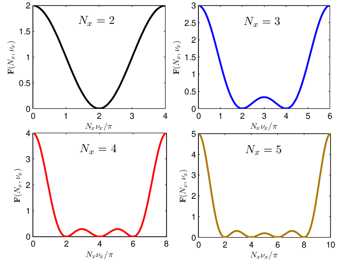
As we can see from the above discussion, in all three cases of the corollary the value of is the one that maximizes . So, to complete the proof we now prove that this value is indeed . Denoting , as per (2) and (39), for we have
| (41) |
For , we have . Then, following (41) we have
| (42) |
where is defined as
It is straightforward to prove that the maximum value of is , which is achieved for . This is also confirmed by Fig. 2, where we plot versus for different value of . As such, is maximized when and thus we have (we ignore the negative solutions due to ) in order to maximize . ∎
We note that for we have and . As such, we have and . We denote the secrecy outage probability of the LBB scheme with unknown Eve’s location (i.e., ) as .
Corollary 4
For , the (multiple) solution to (40) is , , in the following cases: (i) when for finite , (ii) when , or (iii) when is unavailable at Alice.
Proof:
Following similar arguments to those used in the proof of Corollary 3, we know that is to minimize for all three cases in Corollary 4. The value of is given by
| (45) |
where . We note that the minimum value of is achieved when for , which is also confirmed by Fig. 2. As such, is minimized when for , and thus we obtain Corollary 4. ∎
IV Numerical Results
In this section we present numerical simulations to verify our secrecy performance analysis of the LBB scheme, and examine the impact of different system parameters (e.g., , , , and ) on the LBB scheme. To better illustrate the gains obtained by our scheme, we will also present simulations of the secrecy performance of the NB (non-beamforming) scheme. This latter scheme represents the case when an isotropic beamforming pattern is produced by Alice (see Appendix A for an analytical analysis of this scheme). To conduct simulations, we deploy Bob and Eve at specific locations and then map such locations into and , respectively. Such a mapping is based on Alice’s transmit power (i.e., ) and path loss exponents of the main channel and the eavesdropper’s channel (i.e., and ). For presentation convenience, we only specify the values of and adopted in our following simulations. We note that in the following figures we use “Theo” and “Simu” as the abbreviations of “Theoretic” and “Simulated”, respectively.

In Fig. 3 we first verify our derived secrecy outage probabilities for Nakagami fading channels. To this end, we generate channel realizations as per the Nakagami fading channel, where we have set , , , and , where and . The theoretic secrecy outage probability of the LBB scheme, , and the secrecy outage probability of the NB scheme, denoted as , are obtained through (25) and (51), respectively, where relevant infinite series are truncated at 100. In this figure, we observe that the theoretic and precisely match the simulated and , respectively. This confirms the correctness of our derived secrecy outage probabilities.

Recall that for mathematical convenience, our analysis approximates a Rician channel with a Nakagami channel. To see the effect of this, in Fig. 4 we again plot the secrecy outage probabilities of the LBB scheme and the NB scheme, but this time for specific Rician fading channels. In this figure, we observe that the simulated minimum secrecy outage probability of the LBB scheme, , and the secrecy outage probability of the NB scheme, , match extremely well the theoretic and , respectively, thus confirming the validity of our channel approximation. We note that we have set very close to in Fig. 4 (i.e., and ). The gap between and can even be larger when is not so close to .

In Fig. 5, we plot the minimum secrecy outage probability of the LBB scheme, , versus different values of . Again we observe that the theoretic matches extremely well the simulated , which again confirms the validity of our analysis. Fig. 5 is also useful in that it more visually represents how the minimum secrecy outage probability of the LBB scheme depends on the locations of Bob and Eve. For example, is maximized when . In the simulations to obtain Fig. 5, we also observe that the optimal beamforming direction shifts away from as approaches to .
In Fig. 6, we examine the secrecy outage probability of the LBB scheme without knowing Eve’s location, . As per Corollary 3, we know that when Eve’s location is unavailable at Alice. In Fig. 6 we also compare the the solution with no information on Eve’s location to the NB scheme. To conduct a fair comparison with the NB scheme, we assume Eve’s location is uniformly distributed on a circle centered at Alice, i.e., uniformly distributes between and , . We then average over to obtain the average secrecy outage probability, denoted as . As expected, we observe that is lower than , which demonstrates that the LBB scheme still outperforms the NB scheme on average, even when Eve’s location is unavailable at Alice. This is due to the fact that the LBB scheme improves the quality of the main channel based on Bob’s location, which on average reduces the secrecy outage probability. However, the most important result obtained from the simulations of Fig. 6 is that the secrecy outage probability of the LBB scheme without Eve’s location increases (e.g., by approximately a factor of 5 for dB) relative to that of the LBB scheme with Eve’s location. This quantifies the value of the location information of Eve to the beamformer solution.

It is worth mentioning how relaxations of some key assumptions we have made impact the results presented here. Of course, in reality it will never be the case that all reported locations, all map information, and all path loss exponents are known with zero error. Errors in these quantities are intermingled in the sense that an error in one leads to an error in another. We have attempted to encompass such correlated errors in a range of additional simulations. Our general result is that a percentage error of in any of these inputs leads to an approximately percentage error in our reported outage probabilities. For anticipated error inputs, we can therefore say that our analysis remains reasonably accurate.
Finally, although outside the spirit of our low-complexity LBB scheme, it is perhaps worth discussing the gains to be made when the full CSI information of the main channel is made available to Alice (where the transmission scheme is named as the full-CSI scheme). If Eve’s location is also available at Alice in the full-CSI scheme, the full-CSI scheme will of course outperform the LBB scheme for any values of system parameters. For example, under the simulation settings of Fig. 4, the secrecy outage probability of this full-CSI scheme with Eve’s location is lower than that of the LBB scheme for dB and dB (determined from simulations). If Eve’e location is unavailable at Alice (in both schemes) then the full-CSI scheme outperforms the LBB scheme by for dB and dB under the same simulation setting of Fig. 6 (determined from simulations and analysis). For completeness, the secrecy performance analysis of the full-CSI scheme is given in Appendix B.
V Conclusions
We proposed and analyzed a novel beamforming scheme in the wiretap channel where both the main channel and the eavesdropper’s channel are subject to Rician fading. Our new LBB scheme solely requires as inputs the location information of Bob and Eve, and does not require the CSI of the main channel or the eavesdropper’s channel. We derived the secrecy outage probability of the LBB scheme in a closed-form expression valid for arbitrary values of and . We then determined the optimal location-based beamformer that minimizes the secrecy outage probability. Comparisons with a range of other schemes were then carried out so as to better understand the performance gains offered by our location-based solution. The work we presented will be important for a range of application scenarios in which Rician channels are expected to be dominant and where location information of potential users and adversaries are known.
Appendix A Secrecy Performance of the NB Scheme
In the NB scheme, Alice distributes her total transmit power uniformly among the orthogonal independent transmit directions (i.e., the covariance matrix of is ) [23, 24]. Then, the SNR at Bob is given by [23, 24]
| (46) |
Interpreting Rician fading as a special case of Nakagami fading, the pdf of can be approximated by
| (47) |
We assume that Eve applies MRC to combine the received signals at different antenna elements. As such, the SNR at Eve is given by
| (48) |
where is the eigenvector for the largest eigenvalue of . The theoretical expression for the distribution of has been derived in [25]. However, this expression is too complicated to be used for further analysis. To make progress, we adopt the simple approximation for the pdf of proposed in [26]. As such, the pdf of can be approximated by
| (49) |
where is the mean of the per-branch largest eigenvalue (i.e., ). The value of can be approximated by[26]
| (50) |
We note that we have for arbitrary when .
Following a similar procedure to that used in deriving in Theorem 1, the secrecy outage probability of the NB scheme is derived as
| (51) |
As per (51), we can see that the secrecy outage probability of the NB scheme is independent of and . However, (51) is a function of and , which are dependent on and , respectively. We note that the secrecy diversity order of the NB scheme is , which is the full secrecy diversity order. Also, following a similar procedure to that used in deriving in Corollary 2, the probability of non-zero secrecy capacity of the NB scheme is derived as
| (52) | ||||
Appendix B Secrecy Performance of the Full-CSI Scheme
In the full-CSI scheme, Alice knows the CSI of the main channel (Bob feeds back the CSI to Alice), but Alice does not know the CSI of the eavesdropper’s channel or Eve’s location. Then, Alice adopts as the beamformer to maximize the SNR of the main channel [27, 24] in order to minimize the secrecy outage probability. The SNR at Bob of the full-CSI scheme is given by [27, 24]
| (53) |
Again using the Nakagami fading to approximate the Rician fading, the pdf of can be approximated by
| (54) |
We assume that Eve knows by eavesdropping on the feedback from Bob to Alice. We also assume that Eve knows that Alice adopts as the beamformer. Assuming that Eve applies MRC to combine the received signals at different antenna elements, the SNR at Eve is given by
| (55) |
where . In order to derive the pdf of , we next first derive the pdf of . As per (1) and (3), we have
| (56) |
where
To make progress, we make the following approximation
| (57) |
We note that in (57) is deterministic and is a circularly-symmetric complex Gaussian random variable. As such, follows a Rician distribution. Following (57), we have
and
Then, the Rician -factor of is given by
| (58) |
Following (57), we also have
| (59) |
Then, the pdf of can be approximated by
| (60) |
where . Since are independent from each other, the pdf of can be approximated by
| (61) |
Following a similar procedure to that used in deriving in Theorem 1, the secrecy outage probability of the full-CSI scheme is then derived as
| (62) | ||||
As per (62), we know that the secrecy outage probability of the full-CSI scheme is dependent on the locations of both Bob and Eve. This means that we require Bob and Eve’s locations for the secrecy performance analysis of the full-CSI scheme. The locations of both Bob and Eve are not only required by the LBB scheme. We note that the secrecy diversity order the full-CSI scheme is also (full diversity order). Again following a similar procedure of deriving in Corollary 2, the probability of non-zero secrecy capacity of the full-CSI scheme is derived as
| (63) | ||||
References
- [1] Y.-S. Shiu, S. Y. Chang, H.-C. Wu, S. C.-H. Huang, and H.-H. Chen, “Physical layer security in wireless networks: A tutorial,” IEEE Commun. Mag., vol. 18, no. 5, pp. 66–74, Apr. 2011.
- [2] C. E. Shannon, “Communication theory of secrecy systems,” Bell Syst. Techn. J., vol. 28, no. 4, pp. 656–715, Oct. 1949.
- [3] A. Wyner, “The wire-tap channel,” Bell Syst. Techn. J., vol. 54, no. 8, pp. 1355–1387, Oct. 1975.
- [4] S. Goel and R. Negi, “Guaranteeing secrecy using artificial noise,” IEEE Trans. Wireless Commun., vol. 7, no. 6, pp. 2180–2189, Jun. 2008.
- [5] A. Khisti and G. W. Wornell, “Secure transmission with multiple antennas–Part II: The MIMOME wiretap channel,” IEEE Trans. Inf. Theory, vol. 56, no. 11, pp. 5515–5532, Nov. 2010.
- [6] X. Zhou and M. R. McKay, “Secure transmission with artificial noise over fading channels: Achievable rate and optimal power allocation,” IEEE Trans. Veh. Technol., vol. 59, no. 8, pp. 3831–3842, Oct. 2010.
- [7] A. Mukherjee and A. L. Swindlehurst, “Robust beamforming for secrecy in MIMO wiretap channels with imperfect CSI,” IEEE Trans. Signal Process., vol. 59, no. 1, pp. 351–361, Jan. 2011.
- [8] N. Yang, P. L. Yeoh, M. Elkashlan, R. Schober, and I. B. Collings, “Transmit antenna selection for security enhancement in MIMO wiretap channels,” IEEE Trans. Commun., vol. 61, no. 1, pp. 144–154, Jan. 2013.
- [9] S. Yan, N. Yang, R. Malaney, and J. Yuan, “Transmit antenna selection with Alamouti coding and power allocation in MIMO wiretap channels,” IEEE Trans. Wireless Commun., vol. 13, no. 3, pp. 1656–1667, Mar. 2014.
- [10] F. Rusek, D. Persson, B. K. Lau, E. G. Larsson, T. L. Marzetta, O. Edfors, and F. Tufvesson, “Scaling up MIMO: opportunities and challenges with very large arrays,” IEEE Signal Proces. Mag., vol. 30, no. 1, pp. 40–46, Jan. 2013.
- [11] E. G. Larsson, F. Tufvesson, O. Edfors, and T. L. Marzetta, “Massive MIMO for next generation wireless systems,” IEEE Commun. Mag., vol. 52, no. 2, pp. 186–195, Feb. 2014.
- [12] T. L. Marzetta, “Noncooperative cellular wireless with unlimited numbers of base station antennas,” IEEE Trans. Wireless Commun., vol. 9, no. 11, pp. 3590–3600, Nov. 2010.
- [13] H. Yin, D. Gesbert, M. Filippou, and Y. Liu, “A coordinated approach to channel estimation in large-scale multipleantenna systems,” IEEE J. Sel. Areas Commun., vol. 31, no. 2, pp. 264–273, Feb. 2013.
- [14] J. Li and A. P. Petropulu, “Ergodic secrecy rate for multiple-antenna wiretap channels with Rician fading,” IEEE Trans. Inf. Forensics Security, vol. 6, no. 3, pp. 861–867, Sep. 2011.
- [15] N. S. Ferdinand, D. Benevides da Costa, and M. Latva-aho, “Physical layer security in MIMO OSTBC line-of-sight wiretap channels with arbitrary transmit/receive antenna correlation,” IEEE Wireless Comm. Lett., vol. 2, no. 5, pp. 467–470, Oct. 2013.
- [16] S. Yan and R. Malaney, “Line-of-sight based beamforming for security enhancements in wiretap channels,” in Proc. ICITCS2014 IEEE, Oct. 2014, pp. 218–221.
- [17] J.-A. Tsai, R. Buehrer, and B. D. Woerner, “BER performance of a uniform circular array versus a uniform linear array in a mobile radio environment,” IEEE Trans.Wireless Comm., vol. 3, no. 3, pp. 695–700, May 2004.
- [18] G. Taricco and E. Riegler, “On the ergodic capacity of correlated Rician fading MIMO channels with interference,” IEEE Trans. Inf. Theory, vol. 57, no. 7, pp. 4123–4137, Jul. 2011.
- [19] X. Zhou, M. R. McKay, B. Maham, and A. Hjørungnes, “Rethinking the secrecy outage formulation: A secure transmission design perspective,” IEEE Commun. Lett., vol. 15, no. 3, pp. 302–304, Mar. 2011.
- [20] A. Goldsmith, Wireless Communications. Cambridge, U.K.: Cambridge Univ. Press, 2005.
- [21] B. Fisher and A. Kman, “Some results on the Gamma function for negative integers”, Appl. Math. Inf. Sci., vol. 6, No. 2, pp. 173-176, May 2012.
- [22] I. S. Gradshteyn and I. M. Ryzhik, Table of Integrals, Series and Products, 7th ed., Academic, San Diego, CA, 2007.
- [23] E. Telatar, “Capacity of multi-antenna gaussian channels,” Eur. Trans. Telecommun., vol. 10, no. 6, pp. 585–596, Nov. 1999.
- [24] V. Annapureddy, D. Marathe, T. Ramya, and S. Bhashyam, “Outage probability of multiple-input single-output (MISO) systems with delayed feedback,” IEEE Trans. Commun., vol. 57, no. 2, pp. 319–326, Feb. 2009.
- [25] M. Kang, and M.-S. Alouini, “Largest eigenvalue of complex Wishart matrices and performance analysis of MIMO MRC systems,¡± IEEE J. Selec. Areas Commun., vol. 21, no. 3, pp.418–426, Apr. 2003.
- [26] T. Taniguchi, S. Sha, Y. Karasawa, and M. Tsuruta, ¡°Approximation of Largest Eigenvalue Distribution in Rician MIMO Channels,¡± in Proc. IEEE PIMRC, Sep. 2007, pp. 1–5.
- [27] E. Biglieri, G. Caire, and G. Taricco, “Limiting performance of blockfading channels with multiple antennas,” IEEE Trans. Inf. Theory, vol. 47, no. 4, pp. 1273–1289, May 2001.