An aerogel Cherenkov detector for multi-GeV photon detection with low sensitivity to neutrons
Abstract
We describe a novel photon detector which operates under an intense flux of neutrons. It is composed of lead-aerogel sandwich counter modules. Its salient features are high photon detection efficiency and blindness to neutrons. As a result of Monte Carlo (MC) simulations, the efficiency for photons with the energy larger than 1 GeV is expected to be higher than 99.5% and that for 2 GeV/ neutrons less than 1%. The performance on the photon detection under such a large flux of neutrons was measured for a part of the detector. It was confirmed that the efficiency to photons with the energy >1 GeV was consistent with the MC expectation within an 8.2% uncertainty.
PTEP-subject
xxxx, xxx1 Introduction
An electromagnetic sampling calorimeter is one of the most popular detectors for detecting photons in high energy physics. It is usually composed of alternate layers of high-Z converters and active materials sensitive to electrons and positrons. Incident photons produce electromagnetic showers in the converter and their energies are determined in the active layers.
In this paper, we describe a novel photon detector with lead-aerogel sandwich used under an intense flux of neutrons. We choose aerogel Cherenkov radiation as an sensing process so that it is insensitive to heavier particles. The detector is being used in a rare decay experiment[1, 2] at the J-PARC Main Ring (MR)[3]. The experiment, named KOTO, aims to observe the CP-violating decay mode of with a sensitivity exceeding the standard model prediction ([4]). An intense neutral kaon beam is needed to achieve the sensitivity. The beam contains large amounts of photons and neutrons as well as s with typical energies of 10 MeV, 1.4 GeV and 2 GeV, respectively. Rates of the photons and neutrons are expected to be around 600 MHz each with the designed beam condition. Figure 1 shows a cross-sectional view of the KOTO detector assembly. The signature of the decay is a pair of photons from and no other visible particles. The two photons from the are detected with an electromagnetic calorimeter (CsI in Fig. 1) placed downstream of an evacuated decay volume. A number of veto counters surrounding the decay volume hermitically ensure the existence of no other visible particles at the same time. The major background is expected to come from the decay , in which two out of the four photons escape detection. In order to suppress this type of background, photon detection with high efficiency is essential. This requirement is also true for photons escaping into the beam direction, and the energy of these photons ranges 100 MeV-5 GeV. Thus, an efficient photon detector which works inside the beam with a large flux of neutrons is needed. The crucial feature for the photon detector used in such an intense beam is blindness to neutrons, which is to reduce single counting rates and overveto probabilities of the signal events. Various requirements on the detector, including the next two, were evaluated by Monte Carlo (MC) simulations:
- •
The efficiency is >99.5% for photons with the energy of 1 GeV or greater.
- •
The efficiency is <1% for neutrons with the momentum of 2 GeV/.
In Sec. 2, we report various design studies to satisfy these requirements, including results of test experiments with positron and proton beams for verification of the detector response and tuning of the simulation. In Sec. 3, the performance on photon detection in the neutral beam was evaluated for the partially-installed detector in the KOTO experimental area. We add an appendix to describe a measurement of the transmittance of aerogel radiators, which provided important parameters concerning the light yield.

2 Design and expected performance
In this section, we first explain the basic concepts of the detector and describe its components. Next, results of two test experiments with positrons and protons are reported. Finally, we present results of simulation studies on the performance of the designed detector.
2.1 Basic design
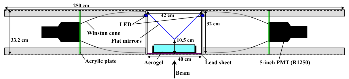
The detector, named BHPV (Beam Hole Photon Veto), is placed at the most downstream part of the KOTO detector assembly as shown in Fig. 1. It is composed of 25 layers of modules along the beam. The structure of a single module is shown in Fig. 2. The main part of the module consists of a lead converter and an aerogel radiator as well as light collecting mirrors and photomultiplier tubes (PMTs).
Design concepts
We chose a lead-aerogel sandwich counter as the module. Photons are detected through Cherenkov radiation of the converted electrons and positrons in the aerogel, which is known to have a small index of refraction ranging between 1.007-1.13. This enables us to reduce sensitivity to neutrons since they tend to produce slow particles which yield no or less Cherenkov light than .
In order to achieve high photon efficiency, optimization of the converter and radiator thicknesses and the refractive index of the aerogel is important. In general, a large number of sampling is required because each converter should be thin enough to reduce shower particles stopping inside the converter and the total thickness should be large enough to ensure conversion of photons into showers. In our case, the total converter thickness of 10 X0 and 25 samplings are adopted. The refractive index of aerogel is chosen as by optimizing the photon efficiency and neutron blindness.
The arrayed configuration along the beam has an additional merit of reducing neutron sensitivity. We note that electromagnetic showers by high energy photons tend to develop into the forward direction while secondary particles such as protons and pions produced by neutron interactions have more isotropic angular distributions. Thus, by defining photons as the events with hits in three or more consecutive modules, we can remove neutron events substantially. Contribution from photons with the energy smaller than 50 MeV in the beam can also be reduced by this requirement. Quantitative results of studies, performed with MC simulations, can be found in Sec. 2.4. In the following, we describe the structure of a single module in more detail.
Structure of a single module
Each single module consists of a lead sheet and aerogel tiles followed by a light collection system and PMTs. The thickness of the lead sheet is 1.5-3.0 mm. Two types of aerogel tiles with different sizes and optical qualities are used. They are named type-M and type-A as listed in Table 1. Several layers of type-M (type-A) tiles are stacked into () grid in order to cover the transverse size of 300-mm-square, oversizing the actual neutral beam of 200-mm-square to detect diverging photons from decays. These tiles are wrapped with a thin polyvinylidene chloride sheet, whose transmittance is 90% for visible light, to maintain their rigidity. The optical system has two identical arms, each of which consists of a flat mirror, a Winston cone[5] for collecting light, and a 5-inch PMT. The advantages of the dual readout system include efficient and uniform light collection. In addition, single counting rates are cut in half, alleviating possible performance deterioration under high rate operation. The flat mirror is made of a 0.75-mm thick aluminum sheet coated by an anodizing method. The reflectivity is 85% over the visible light region. The Winston cone (480-mm-long) is designed to funnel the Cherenkov light from the input aperture of 300 mm in diameter into the output aperture of 120 mm. It is made of an aluminum sheet by deep-draw processing; its inner surface is coated with aluminum by vapor deposition. The average reflectivity is 85% for visible light. The 5-inch PMT, Hamamastu R1250[6], has a bialkali photocathode with borosilicate glass. Its quantum efficiency peaks around the wavelength of 400 nm with value of 20%, according to its catalog information. Light emitting diodes (LEDs) are installed for calibration of the PMTs.
| Type | Refractive | Dimensions | Configuration | Transmission length [cm] |
|---|---|---|---|---|
| index () | [mm3] | of stacking | (at the wavelength of 400 nm) | |
| M | 1.03 | 5.07 | ||
| A | 1.03 | 3.35 |
Note: The transmission length, defined as the path length at which the original intensity is reduced to , is calculated with Eq. (11) using the measured parameters. See Appendix for detail.
Arrayed configuration of modules
Twenty-five modules are arranged along the beam axis. Thickness of the lead and aerogel radiator for each module are shown in Fig. 3. This configuration, used in the simulation studies in Sec. 2.4, is referred as the reference configuration. They are optimized according to experimental conditions such as beam intensity in order to keep the photon detection efficiency high and the single counting rates as low as possible. For example, thinner lead sheets and aerogel in the upstream modules, as in the reference configuration, help to reduce the counting rates in these modules where high rates are expected.
2.2 Photoelectron yield measurement with a positron beam
The average number of observable photoelectrons (p.e.) produced by a single relativistic electron traveling through the aerogel radiator is the most important quantity. The value was obtained by the “calibration experiment” with a positron beam. The experiment was performed using a 600 MeV/ positron beam at the Laboratory of Nuclear Science11 1 Presently the Research Center for Electron Photon Science of Tohoku University, Japan in 2009. Five layers of type-M aerogel tiles in Table 1 were used in this measurement. Figure 4 shows a schematic view of the experimental layout. Plastic scintillation counters were placed in both the upstream and downstream of the detector module. The trigger signal was formed essentially by the coincidence signals of T1 and T4 counters, both of which had dimensions of 1 cm 1 cm in cross section and 0.5 cm in thickness.


Figure 5 shows the photoelectron yields as a function of the horizontal beam position. In the measurement, an output of each PMT was converted to the number of photoelectrons using an LED calibration data. Results of corresponding MC simulations are shown in the same figure with lines, where ray tracing was performed for individual Cherenkov light produced in the aerogel. Here, we took into account various loss factors such as geometrical acceptance and reflectivity of the optical system, quantum efficiency of the PMT, and measured transmittance of the aerogel tiles22 2 Detail of the measurement is in Appendix.. The dips around cm are due to boundaries between the aerogel tiles. The simulation successfully reproduces the uniform photoelectron yield over the entire region in the data. The absolute scale of the simulation was corrected so that the average photoelectron yield agreed with that of the data. This scale factor is referred to as the “calibration factor” and is found to be 0.55 in this measurement. The origin of this correction is considered to be due to uncertainty in the quantum efficiency of the PMT and deterioration of the aerogel surface during transportation and handling. In fact, fine fragments produced by frictions of tiles were observed on the surface during the measurement. It was likely that they caused an additional loss of the photoelectron yield.
2.3 Measurement of hadronic response
In this section, we describe test results with a proton beam. The purposes are to validate the MC simulation for hadronic interactions and to examine experimentally the detector response to hadrons.

The experiment was performed at the 12 GeV Proton Synchrotron of High Energy Accelerator Research Organization (KEK), Japan in 2002. Figure 7 shows its schematic layout. Figure 7 shows the test module with one 5-inch PMT and a parabola mirror as an optical system. A 20-mm-thick lead converter and five aerogel tiles with the same dimensions as type-M33 3 Aerogel used in this measurement had different optical characteristics from both of type-M and type-A. Transmittance and calibration factor were separately measured for this aerogel. were placed in the module. A much thicker converter than that in the reference configuration in Sec. 2.1 was used to enhance hadronic interactions. The trigger signal was formed by a coincidence signal from the time-of-flight counters (TOF1 and TOF2) and two 1-cm-wide mutually orthogonal counters (F1x and F1y). Particle identification was made by time-of-flight information measured by TOF1 and TOF2.
Figure 8 shows the results of the measurement with MC expectation; the efficiency with the threshold of 1.75 p.e. is plotted as a function of the proton momentum. Note that the efficiency obtained in this measurement is for a single test module. In spite that a proton itself dose not generate Cherenkov light in this momentum range, it can make a signal in the module through the generation of knock-on electrons and secondary particles such as s. In addition, the scintillation light from nitrogen in the air also makes contribution[7]. The agreement between the data and MC in Fig. 8 shows that the response of this detector to protons is well-understood. These results validate our MC simulations on the neutron blindness of the detector.
2.4 Expected performance
In this section, we present the expected performance studied by MC simulations. We have adopted the GEANT4 simulation codes[8]. We focus on the photon efficiency and neutron blindness.
Condition of the simulation
The reference configuration described in Sec. 2.1 was employed in the simulation study. The type-A aerogel, which are used in the KOTO physics run, was assumed. Transmittance and calibration factors, separately measured for this aerogel, were implemented. The simulation procedure is as follows. Photons with various energies were injected uniformly over the detector upstream surface of 250-mm-square. When tracks in the electromagnetic showers traversed the aerogel radiator, Cherenkov light was emitted and the rays were traced from the radiator to the PMT cathode. The amount of the Cherenkov light at the PMT was converted to the number of photoelectrons by using the calibration factor. The same procedures were applied until all the shower particles exited from the entire detector or lost their energy completely.


Photon efficiency
The following algorithm was adopted to identify photons. In a single module, a hit was recognized when the output from either or both of the two PMTs exceeded a 1.5 p.e. threshold. If three or more consecutive hits were recorded, then the event was identified as a photon. Black solid circles in Fig. 10 show the inefficiency as a function of the incident photon energy. The simulation shows that the detector satisfies the photon efficiency requirement, 99.5% for >1 GeV.
Neutron blindness
Estimation of the neutron efficiency proceeded in the same way as the photon efficiency. In this case, neutrons were injected, and hadronic showers were produced in the lead converter. We used the hadron package of QGSP to simulate the neutron interactions. All the charged particles were tracked and Cherenkov light was created when the momentum was above the Cherenkov threshold. The event identification algorithm was the same as in the photon case. Figure 10 shows the neutron efficiency as a function of incident neutron momentum. The efficiency increases monotonically with the momentum, and remains below 1% for 2 GeV/ neutrons, satisfying the requirement specified in Sec. 1.
Different algorithms may lead to different photon inefficiencies and neutron efficiencies. Examples of such studies are shown in Fig. 10 and Fig. 10. If the number of required consecutive hits is lowered, the efficiency for low energy photons increases, but the efficiency for neutrons also increases. These conditions can be optimized according to specific experimental situations.
3 Photon identification in the neutral kaon beam
As mentioned in Sec. 1, a part of the entire BHPV detector was installed in the experimental area together with other KOTO detectors. This partial detector consists of 12 modules, and was loaded with 58-mm-thick type-A tiles and lead converters with different thickness: five 1.5-mm (No.1--5), five 3-mm (No.6--10) and two with no plates (No.11--12)44 4 Since the identification of a photon signal requires hits in three or more consecutive modules, lead in the last two modules dose not contribute to the total thickness effectively. This is why the modules No. 11 and No. 12 do not have lead converters.. Outputs from this detector were recorded by waveform digitizers of 500 MHz sampling, which were custom-built for the KOTO experiment[9]. Multiple hits in a single counter were distinguished correctly even under the high-rate environment. We present analysis results of the 100-hour data obtained in the first physics data taking in May, 2013. The beam power of the J-PARC MR was 24 kW, which corresponds to the average neutron and photon rates of 100 MHz and 170 MHz55 5 The rates are with the kinetic energy larger than 1 MeV., respectively, from the MC simulation. We focus on the detector response to high energy photons from decays with the accompanied neutron and photon fluxes.
3.1 Photon tagging with decay samples
There were six photons in the decay. In the analysis, we required five out of the six photons to hit the CsI calorimeter. Kinematics of the decay allowed the reconstruction of the “missing” photon with a two-fold ambiguity. This “tagged photon” technique was used to evaluate the performance of the BHPV with the collected data in the KOTO experiment. We compared data with MC to validate the performance. From the MC simulation, the “missing photon,” denoted as below, has an geometric acceptance of 3% in the direction of the BHPV. Details of the CsI calorimeter can be found elsewhere[2, 10]. We started with the selection of the five reconstructed photons. For any two photons, when we assumed they were from decay, the longitudinal vertex position was calculated:
| (1) |
where is the mass, is the opening angle, and , were the photon energies. We further assumed the transverse position of the to be at the beam-line. Out of the five photons, there were 15 possible combinations to reconstruct two decays. For each of these 15 combinations, there were two vertices. We chose the correct combination by requiring the two vertices to be the same (best fit) so that it is the common vertex of the decay66 6 We calculated for each combination, and chose the smallest one. Here denotes each candidate, () is its vertex position (resolution), and is the weighted-mean of the two vertex positions.. With the decay vertex known, momentum of the third was calculated. We denoted and as the two photons from the third :
| (2) | |||||
where , , and were energies of the third , and , respectively. , , and () are the -th components of the momenta. For the three unknowns of momenta, the two transverse components (, ) were determined assuming that the parent has no transverse momentum. Equation (2) is thereby quadratic for . For the two solutions of , we obtained two invariant masses. The solution with the larger (smaller) was called the “forward”(“backward”) solution and the corresponding mass was denoted as ().
We required , because a simulation study showed that the forward solution was correct for most of the cases in which the hit the BHPV detector. Events with were rejected to reduce unnecessary backward solution events. Comparison of the distribution between the data and MC is shown in Fig. 11. The MC result was normalized with the number of events after the cuts on the reconstructed mass. The MC well reproduced the data, though the distribution had no clear peak around the nominal mass due to events with incorrect photon combinations. When we selected the events with proper photon combinations and going into the BHPV in the simulation, the distribution had a peak around the nominal mass as the blue histogram in Fig. 11. The background contamination, mainly from the and decays with the subsequent Dalitz decay (), was estimated to be 9.8%.
As a reference, events where all the six photons from the decay hit the calorimeter were reconstructed. These events were called the “6” events, and the procedure was almost the same with that in 5 events except the assumption that all 3 came from the common decay vertex. With the same normalization factor as in Fig. 11, the number of the 6 events was found to be consistent between the data and MC within the statistical uncertainty of 0.5%.


3.2 BHPV photon response
Now we examine the response of the BHPV detector using the and 6 events. A photon hit in the detector was identified as three or more consecutive modules with the outputs exceeding the 2.5 p.e. threshold in either or both of the left and right PMTs. Figure 12 shows the timing distribution of the photon hits in the BHPV detector with respect to the timing determined by the CsI calorimeter77 7 The BHPV hit timing was defined as the hit times averaged over the modules with hits after correcting time of propagation of the shower particles module by module. The CsI hit timing was the weighted average of the photon hit times where the weight is given by the photon energy. Correction due to the time-of-flight between a decay vertex to hit positions was applied.. For the events, shown with the blue bars in Fig. 12 (left), there should be only accidental hits in the BHPV detector. The periodic distribution seen in these hits reflects the beam bunch structure in the slowly-extracted beam from the J-PARC MR. On the other hand, for the events shown by the red open squares, a sharp peak is observed on top of the accidental hits. Figure 12 (right bottom) shows the timing distribution of the events after subtracting the distribution of the accidental hits in Fig. 12 (right top). The value from the gaussian fit was found to be ns. This is a clear evidence that the missing photons tagged by the events were successfully detected by the BHPV detector.
We compared the number of events within 7.5 ns of the peak in the timing distribution of the 5 events between the data and MC. Figure 13 (left) shows the distribution of the total photoelectron yields observed by the hit modules in these events. The total photoelectron yield was obtained by summing the outputs over the modules which recorded hits88 8 The output from a module was defined as the sum of the outputs exceeding 2.5 p.e. in the left and right PMTs. in three or more consecutive modules. For the the data and MC, distributions of the accidental hits were subtracted. The data and MC distributions agree. As expected, the photoelectron yields increase with the energies of the (the missing photon). The energy distribution of the going into the BHPV direction in the simulation is shown in Fig. 13 (right). We now focus on the events with the total photoelectron yield greater than 200. The and were defined as the numbers of such events in the real data and the MC simulation, respectively. In addition, we define . Since the MC simulation shows that these events are mainly from the with MeV hitting the detector (90.3%), is a good measure of the detector response to high energy photon. If the detector works as expected in the MC simulation, gets close to 1. Based on Fig. 13, , where the first and second errors represent the statistical and the systematic uncertainties, respectively. A summary of the systematic errors is presented in Table 2. The MC reproducibility of the BHPV was evaluated by comparing the efficiency of each selection cut related to the BHPV between the data and MC. For the other error sources, each condition was shifted within its uncertainty in the MC simulations and changes of the event ratio with the going to the BHPV were considered as the error.
| Error source | Relative error [%] |
|---|---|
| MC reproducibility on BHPV | 3.80 |
| momentum spectrum | |
| Beam position | 0.15 |
| Calorimeter energy resolution | 0.49 |
| Calorimeter position resolution | 4.98 |
| Detector alignment | 1.50 |
| Total |
Finally, the detection efficiency for high energy photons was estimated from the value obtained above. The efficiency was defined as
| (3) |
where and were the numbers of events with the detected and incident in the BHPV detector, respectively, when its energies was larger than 1 GeV. We assumed
| (4) |
and evaluated with the simulation (). This assumption allows Eq. (3) to be deformed as follows:
| (5) | |||||
The efficiency in the MC simulation, written as , was calculated to be . Here, the inefficiency of 6% mainly came from lack of the total radiation length and would be reduced by adding modules to have enough thickness of the lead converter. From Eq. (5), the efficiency for high energy photons was obtained as .
The value, which indicates the reproducibility of MC, is consistent with 1 within the error. We concluded that high energy photons are successfully detected by this detector as expected even when it was placed in the intense neutral beam. The distribution of the shower-starting module between the data and MC in Fig. 14 confirms further the detector performance. The obtained efficiency, which is close to 1, indicates the excellent performance of the system as a photon veto detector.
4 Summary
In this paper, we have described a novel photon detector used in an intense neutral kaon beam line. The aerogel Cherenkov radiation is adopted for the detection of electromagnetic showers, and blindness to neutrons is expected. According to MC simulations, which have been validated by tests experiments with positrons and protons, efficiencies to photons with the energy larger than 1 GeV and to neutrons with the momentum of 2 GeV/ are >99.5% and <1%, respectively. The detector was partially installed in the first physics run of the KOTO experiment, and performance to high energy photons was evaluated by tagging decay events. It was confirmed the photon detection efficiency expected by the MC simulations was successfully achieved within the 8.2% uncertainty.
Acknowledgment
We would like to express our gratitude to staffs of the KEK Proton Synchrotron and the Laboratory of Nuclear Science for their cooperation in the test beam experiments. We also thank the staff members of the J-PARC accelerator, Hadron Beam groups and the KEK Computing Research Center for their supports in taking and analyzing the physics data. Part of this work was supported by MEXT KAKENHI Grant Numbers 23224007, 18071006, 14046220 and the Japan/US Cooperation Program. Some of the authors were supported by Grant-in-Aid for JSPS Fellows.
Appendix: Aerogel transmittance measurement
The transmittance of aerogel is known to be influenced mainly by two effects; absorption and Rayleigh scattering. According to [11], it can be represented as
| (11) |
where and denote the thickness of aerogel and the wavelength of light, respectively. and are constants. The first (second) exponential represents the absorption (Rayleigh scattering) effect, and and characterize aerogel’s transmittance property.
These constants were measured using the setup shown in Fig. 30. There were five LEDs with different colors, which were irradiated onto the aerogel sample under test through 2-mm-diameter holes. The LEDs and aerogel sample were placed on movable tables controlled by a computer. The transmittance was obtained by comparing light outputs from the main PMT behind the aerogel sample and those without the sample. The stability of the LEDs was monitored by a separate PMT placed near the LEDs. An example of the measurement results is shown in Fig. 30 together with a fit result with Eq. (11). In Table 5, we list the parameters obtained for the type-A and type-M aerogels averaged over many measurements and samples. Combining with the information from the photoelectron calibration experiment, these parameter measurements provide inputs to the simulation studies.
| Type | ||
|---|---|---|
| [cm/m4] | ||
| M | 0.96 | 0.0040 |
| A | 0.972 | 0.00692 |
Note: The parameter is defined as , where is taken to be 1 cm.
References
- [1] J-PARC E14 (KOTO) experimental proposal, http://koto.kek.jp/
- [2] T. Yamanaka, Prog. Theor. Exp. Phys. (2012) 02B006.
- [3] T. Koseki et. al., Prog. Theor. Exp. Phys. (2012) 02B004.
- [4] J. Brod, M. Gorbahn and E. Stamou, Phys. Rev. D83, 034030 (2011).
- [5] Winston R., J. Opt. Soc. Amer., 60, 245 (2004).
- [6] Hamamatsu Photonics K.K., http://www.hamamatsu.com/jp/en/R1250.html.
- [7] H. Morii, et al., Nuclear Instruments and Methods in Physics Research A 26 (2004) 399-408.
- [8] S. Agostinelli, et al., Nucl. Instr. and Meth. A 506 (2003) 250.
- [9] M. Bogdan, J-F. Genat, Y. W. Wah, Real Time Conference (RT), 2010 17th IEEE-NPSS , vol., no., pp.1,2, 24-28 May 2010.
- [10] T. Masuda, Ph.D. thesis, Kyoto University (2014).
- [11] E. Aschenauer et al., Nuclear Instruments and Methods in Physics Research A 440 (2000). 338-347.