\PHyear2014 \PHnumber281 \PHdate17 November \ShortTitleParticle production and centrality in p–Pb \CollaborationALICE Collaboration \ShortAuthorALICE Collaboration
We report measurements of the primary charged particle pseudorapidity density and transverse momentum distributions in p–Pb collisions at TeV, and investigate their correlation with experimental observables sensitive to the centrality of the collision. Centrality classes are defined using different event activity estimators, i.e. charged particle multiplicities measured in three different pseudorapidity regions as well as the energy measured at beam rapidity (zero-degree). The procedures to determine the centrality, quantified by the number of participants (), or the number of nucleon-nucleon binary collisions (), are described. We show that, in contrast to Pb–Pb collisions, in p–Pb collisions large multiplicity fluctuations together with the small range of participants available, generate a dynamical bias in centrality classes based on particle multiplicity. We propose to use the zero-degree energy, which we expect not to introduce a dynamical bias, as an alternative event-centrality estimator. Based on zero-degree energy centrality classes, the dependence of particle production is studied. Under the assumption that the multiplicity measured in the Pb-going rapidity region scales with the number of Pb-participants, an approximate independence of the multiplicity per participating nucleon measured at mid-rapitity of the number of participating nucleons is observed. Furthermore, at high- the p–Pb spectra are found to be consistent with the pp spectra scaled by for all centrality classes. Our results represent valuable input for the study of the event activity dependence of hard probes in p–Pb collision and, hence, help to establish baselines for the interpretation of the Pb–Pb data.
1 Introduction
Proton–lead collisions are an essential component of the heavy ion programme at the Large Hadron Collider (LHC) [1]. Measurements of benchmark processes in p–Pb collisions serve as an important baseline for the understanding and the interpretation of the nucleus–nucleus data. These measurements allow one to disentangle hot nuclear matter effects which are characteristic of the formation of the quark-gluon plasma (QGP) from cold nuclear matter effects. The latter are the effects due to the presence of the nuclei themselves and not the QGP, for example broadening, nuclear modification of parton densities, and partonic energy loss in cold nuclear matter.
Of particular interest are studies of nuclear effects on parton scatterings at large momentum transfer (hard processes). To this end, the nuclear modification factor defined as the ratio of particle or jet transverse momentum () spectra in minimum bias (MB) p–Pb to those in pp collisions scaled by the average number of binary p–nucleon (p–N) collisions is measured [2]. The latter is given by the ratio of p–N and p–Pb inelastic cross-sections times the mass number . In the absence of nuclear effects, the nuclear modification factor is expected to be unity. In heavy ion collisions, binary scaling is found to hold in measurements of prompt photons [3] and electroweak probes [4, 5], which do not strongly interact with the medium. The observation of binary scaling in p–Pb demonstrates that the strong suppression of hadrons [6], jets [7] and heavy flavour hadrons [8, 9] seen in Pb–Pb collisions is due to strong final state effects. Centrality dependent measurements of the nuclear modification factor , defined as
| (1) |
require the determination of the average for each centrality class.
Moreover, it has been recognised that the study of p–Pb collisions is also interesting in its own right. Several measurements [10, 11, 12, 13] of particle production in the low and intermediate transverse momentum region clearly show that p–Pb collisions cannot be explained by an incoherent superposition of pp collisions. Instead the data are compatible with the presence of coherent [14] and collective [15] effects. Their strength increases with multiplicity indicating a strong collision geometry dependence. In order to corroborate this hypothesis a more detailed characterisation of the collision geometry is needed.
The Glauber model [16] is generally used to calculate geometrical quantities of nuclear collisions (A–A or p–A). In this model, the impact parameter controls the average number of participating nucleons (hereafter referred as “participants” or also “wounded nucleons” [17, 18]), and the corresponding number of collisions . It is expected that variations of the amount of matter overlapping in the collision region will change the number of produced particles, and parameters such as and have traditionally been used to describe those changes quantitatively, and to relate them to pp collisions.
Using the Glauber model one can calculate the probability distributions , where stands for or . Since cannot be measured directly it has to be related via a model to an observable , generally called centrality estimator, via the conditional probability to observe for a given . For each collision system and centre of mass energy, the model has to be experimentally validated by comparing the measured probability distribution to the one calculated from the convolution . Once the model has been validated, for each event class defined by an -interval the average is calculated. In order to unambigously determine , one chooses observables whose mean values depend monotonically on . Note that in p–A collisions the impact parameter is only loosely correlated to . Hence, although one uses traditionally the term centrality to refer to these measurements, the relevant parameters are and .
The procedure described above can be easily extended to several estimators. Of particular interest are estimators from kinematic regions that are causally disconnected after the collision. The measurement of a finite correlation between them unambiguously establishes their connection to the common collision geometry. Typically these studies are performed with observables from well separated pseudorapidity () intervals, e.g. at zero-degree (spectators, slow-nucleons, deuteron break-up probability) and multiplicity in the rapidity plateau.
The use of centrality estimators in p–A collisions based on multiplicity or summed energy in certain pseudo-rapidity intervals is motivated by the observation that they show a linear dependence with or . This is also in agreement with models for the centrality dependence of particle production (e.g. the Wounded Nucleon Model [17, 18]), or also string models like FRITIOF [19]). The total rapidity integrated multiplicity of charged particles measured in hadron–nucleus collisions () at centre of mass energies ranging from 10 to 200 GeV (E178 [20], PHOBOS [21]) is consistent with a linear dependence on : . The ratio of particle pseudorapidity () densities in d–Au and pp collisions exhibits a dependence on , which implies that the scaling behaviour has a strong rapidity dependence with an approximate -scaling at and an approximate scaling with the number of target participants () in the Au-going direction [21]. In d–Au collisions at RHIC ( GeV), the PHENIX and STAR collaborations [22, 23] have used the multiplicity measured in an -interval of width 0.9 centered at (Au-going direction) as a centrality estimator. The multiplicity distribution has been successfully described by the Glauber model assuming - scaling. Finally, in centrality averaged p–Pb collisions at the LHC ( TeV) the primary charged particle pseudorapidity density at scaled by the mean number of participants is found to be consistent with the corresponding value in pp collisions interpolated to the same [24].
At RHIC, the deuteron dissociation probability can be accurately modelled by a Glauber calculation and measured using the zero degree calorimeters in the d-direction [25, 22]. The mean number of participants has been determined for centrality classes obtained with the multiplicity estimator described above and used to calculate the deuteron break-up probability. Inferred and measured probabilities are consistent, demonstrating the correlation between collision geometry and multiplicity, and providing a stringent test for the determination.
Since for example hard scatterings can significantly contribute to the overall particle multiplicity, correlations between high- particle production and bulk multiplicity can also be induced after the collisions and, hence, they are not only related to the collision geometry. Therefore, the use of from the Glauber model to scale cross-sections of hard processes from pp to p–A has to undergo the same scrutiny as the correlation of the centrality estimator to the collision geometry. This is necessary also due to the enhanced role of multiplicity fluctuations in p–A. While the average of centrality estimators vary monotonically with , for a full description of the conditional probability fluctuations of for a fixed have to be taken into account. In Pb–Pb collisions, these multiplicity fluctuations have little influence on the centrality determination. The range of is large and converges with increasing rapidly to a Gaussian with small width relative to the the range of . However, in p–Pb collisions, the range of multiplicities used to select a centrality class is of similar magnitude as the fluctuations, with the consequence that a centrality selection based on multiplicity may select a biased sample of nucleon–nucleon collisions (for a discussion of this effect in d+Au see [22]).
In essence, by selecting high (low) multiplicity one chooses not only large (small) average , but also positive (negative) multiplicity fluctuations leading to deviations from the binary scaling of hard processes. These fluctuations are partly related to qualitatively different types of collisions. High multiplicity nucleon-nucleon collisions show a significantly higher particle mean transverse momentum. They can be understood as “harder” collisions, i.e. with higher 4-momentum transfer squared or as nucleon-nucleon collisions where multiple parton-parton interactions (MPI) take place.
In contrast, a centrality selection that is not expected to induce a bias on the binary scaling of hard processes is provided by the energy measurement with the Zero Degree Calorimeters (ZDC) due to their large -separation from the central barrel detectors. They detect the so-called “slow” nucleons produced in the interaction by nuclear de-excitation processes, or knocked out by wounded nucleons [26, 27]. The relationship of the energy deposited in the ZDC to the number of collisions requires a detailed model to describe the slow nucleon production. A heuristic approach, based on a parameterization of data from low energy experiments, is discussed in the present paper.
We will show that centrality estimators using forward neutron energy and those using central multiplicity give consistent results for and , demonstrating their connection to the collision geometry. Based on the considerations outlined above we study two different procedures for centrality estimation. The first procedure is to determine the centrality with charged particle multiplicity. The collision geometry is determined by fitting the measured multiplicity distribution with the distribution obtained from the Glauber model [16], convolved with a negative binomial distribution (NBD). Due to the possible dynamical bias introduced by the multiplicity selection should in this case not be used to scale hard cross-sections. Additional effort is needed to understand the bias or to extend the Glauber model to include additional dynamical fluctuations. Several possible directions have been discussed, for example Glauber-Gribov fluctuations of the proton size [28] as well as fluctuations of the number of hard-scatterings per collisions due to the impact parameter dependence and purely statistical (Poissonian) fluctuations [29].
The second procedure requires a centrality selection with minimal bias and, therefore, uses the ZDC signal. To relate the ZDC signal to the collision geometry we have developed a heuristic model for slow nucleon emission, based on a parameterization of data from low energy experiments. This heuristic approach however can provide only a model-dependent determination. However, one can study the correlation of two or more observables out of which at least one is expected to scale linearly with . Examples are i) the target-going multiplicity proportional to the number of wounded target nucleons (), ii) the multiplicity at mid-rapidity proportional to the number of participants (), iii) the yield of hard probes, like high- particles at mid-rapidity proportional to . These scalings can be used as an ansatz when calculating based on an event selection using the ZDC.
Both alternatives are discussed in the present paper. The paper is organised as follows. Section 2 describes the experimental conditions, the event selection, and the event characterisation using the multiplicity distributions of charged particles measured in various ranges, or the energy collected in the ZDC. Section 3 describes the centrality determination based on charged particle distributions using an NBD-Glauber fit to extract the average geometrical quantities for typical centrality classes. Section 4 presents a phenomenological model describing the relation of the energy deposited in the ZDC calorimeter and . Section 5 discusses the various effects leading to a bias in the centrality measurements based on particle multiplicity. Section 6 introduces a hybrid method, where we use the ZDC to characterize the event activity, and base the determination of on the assumption that -scaling holds for the central pseudorapidity multiplicity density or -scaling for particle production in the target region. Section 7 discusses the implications of the different choices of a centrality estimator on the physics results, such as the nuclear modification factors, or the pseudorapidity density of charged particles at mid-rapidity. Section 8 summarizes and concludes the paper.
2 Experimental Conditions
The data were recorded during a dedicated LHC run of 4 weeks in January and February 2013. Data have been taken with two beam configurations, by inverting the direction of the two particle species, referred to as p–Pb and Pb–p, respectively, for the situations where the proton beam is moving towards positive rapidities, or vice versa. The two-in-one-magnet design of the LHC imposes the same magnetic rigidity of the beams in the two rings ,implying that the ratio of beam energies is fixed to be exactly equal to the ratio of the charge/mass ratios of each beam. Protons at 4 TeV energy collided onto fully stripped Pb ions at 1.58 TeV per nucleon energy resulting in collisions at TeV in the nucleon–nucleon centre-of-mass system (cms), which moves with a rapidity of in the direction of the proton beam. In the following, we will use the convention that stands for , defined such that the proton moves towards positive , while stands for .
The number of colliding bunches varied from 8 to 288. The proton and Pb bunch intensities were ranging from 0.2 to 6.5 and from 0.1 to 4.4 , respectively. The luminosity at the ALICE interaction point was up to 5 cm−2s−1 resulting in a 10 kHz hadronic interaction rate. The RMS width of the interaction region is 6.3 cm along the beam direction and of about 60 m in the direction transverse to the beam.
The ALICE apparatus and its performance in the LHC Run 1 are described in [30] and [31], respectively. The main detector components used for the centrality determination are: the Silicon Pixel Detector (SPD), two cylindrical layers of hybrid silicon pixel assemblies covering for the inner layer and for the outer layer for vertices at the nominal interaction point, with 93.5% active channels; the Time Projection Chamber (TPC), a large cylindrical drift detector covering ; the VZERO scintillator counters, covering the full azimuth within (VZERO-A) and (VZERO-C); and the Zero Degree Calorimeters (ZDC), two sets of neutron (ZNA and ZNC) and proton (ZPA and ZPC) calorimeters positioned at 112.5 m from the interaction point, with an energy resolution of about 20% for the neutron and 24% for the proton calorimeters.
The p–Pb trigger, configured to have high efficiency for hadronic events, requires a signal in both the VZERO-A and VZERO-C (VZERO-AND requirement). Beam–gas and other machine-induced background collisions with deposited energy above the thresholds in the VZERO or ZDC detectors are suppressed by requiring the signal arrival time to be compatible with a nominal p–Pb interaction. The fraction of remaining beam-related background after all requirements is estimated from control triggers on non-colliding or empty bunches, and found to be negligible.
The resulting event sample corresponds to a so-called visible cross-section of measured in a van der Meer scan [32]. From Monte Carlo simulations we expect that the sample consists mainly of non-single diffractive (NSD) collisions and a negligible contribution of single-diffractive (SD) and electromagnetic interactions. The VZERO-AND trigger is not fully efficient for NSD events. Previous Monte Carlo studies (for details see [24]) have shown that the inefficiency is observed mostly for events without reconstructed vertex, i.e. with no particles produced at central rapidities. Given the fraction of such events in data (1.5%), the corresponding inefficiency was found to be 2.2% with a large systematic uncertainty of 3.1%. Correcting for this inefficiency would mainly concern the most peripheral class (80-100%) where the correction amounts up to 11% 15.5%. For the results reported in this paper, centrality classes have been defined as percentiles of the visible cross-section and the measurements are not corrected for trigger inefficiency.
The centrality determination is performed by exploiting the rapidity coverage of the various detectors. The raw multiplicity distributions measured in the Central Barrel are modelled by assuming particle production sources are distributed according to a NBD. The zero-degree energy of the slow nucleons emitted in the nucleon fragmentation requires more detailed models.
In this context, the main estimators used for centrality in the following are:
-
CL1: the number of clusters in the outer layer of the silicon pixel detector, ;
-
V0A: the amplitude measured by the VZERO hodoscopes on the A-side (the Pb-going side in the p–Pb event sample), ;
-
V0C: the amplitude measured by the VZERO hodoscopes on the C-side (the p-going side in the p–Pb event sample), ;
-
V0M: the sum of the amplitudes in the VZERO hodoscopes on the A- and C-side (V0A+V0C);
-
ZNA: the energy deposited in the neutron calorimeter on the A-side (the Pb-going side in the p–Pb event sample).
3 Centrality from Charged Particle Distributions
3.1 NBD-Glauber Fit

To determine the relationship between charged particle multiplicity and the collision properties, such as the number of participating nucleons , binary pN collisions , or nuclear overlap (), it is customary to use the Glauber Monte Carlo model combined with a simple model for particle production [33, 34, 35, 36, 37]. The method was used in Pb–Pb collisions and is described in detail in [38]. In the Glauber calculation, the nuclear density for Pb is modelled by a Woods-Saxon distribution for a spherical nucleus
| (2) |
with the nucleon density, which provides the overall normalization, a radius of () fm and a skin depth of fm, based on data from low energy electron-nucleus scattering experiments [39]. Nuclear collisions are modelled by randomly displacing the projectile proton and the target Pb nucleus in the transverse plane. A hard-sphere exclusion distance of fm between nucleons is employed. The proton is assumed to collide with the nucleons of the Pb-nucleus if the transverse distance between them is less than the distance corresponding to the inelastic nucleon-nucleon cross-section of mb at TeV, estimated from interpolating data at different centre of mass energies [40] including measurements at 2.76 and 7 TeV [41]. The VZERO-AND cross-section measured in a van der Meer scan [32] was found to be compatible, assuming negligible efficiency and EM contamination corrections, with the Glauber-derived p-nucleus inelastic cross-section (2.1 0.1 b). The Glauber-MC determines on an event-by-event basis the properties of the collision geometry, such as , and , which must be mapped to an experimental observable.
Assuming that the average V0A multiplicity is proportional to the number of participants in an individual p–A collision, the probability distribution of the contributions to the amplitude from each p-nucleon collisions can be described by the NBD, defined as:
| (3) |
where is the gamma function, the mean amplitude per participant and the dispersion parameter is related to the relative width given by . From the closure of the NBD under convolution, it follows that the conditional probability , i.e. repeated convolutions, is equal to .
| System | pp | p–Pb | ||
|---|---|---|---|---|
| Distribution | ||||
| V0A | 9.6 | 0.56 | 11.0 | 0.44 |
| V0M | 25.2 | 0.82 | 23.6 | 1.08 |
| CL1 | 9.8 | 0.64 | 8.74 | 0.76 |
| Centrality (%) | (fm) | (mb-1) | (mb-1) | |||||
|---|---|---|---|---|---|---|---|---|
| 0 - 5 | 3.12 | 1.39 | 0.211 | 0.0548 | 15.7 | 3.84 | 14.7 | 3.84 |
| 5 - 10 | 3.50 | 1.48 | 0.186 | 0.0539 | 14.0 | 3.78 | 13.0 | 3.78 |
| 10 - 20 | 3.85 | 1.57 | 0.167 | 0.0549 | 12.7 | 3.85 | 11.7 | 3.85 |
| 20 - 40 | 4.54 | 1.69 | 0.134 | 0.0561 | 10.4 | 3.93 | 9.36 | 3.93 |
| 40 - 60 | 5.57 | 1.69 | 0.0918 | 0.0516 | 7.42 | 3.61 | 6.42 | 3.61 |
| 60 - 80 | 6.63 | 1.45 | 0.0544 | 0.0385 | 4.81 | 2.69 | 3.81 | 2.69 |
| 80 - 100 | 7.51 | 1.11 | 0.0277 | 0.0203 | 2.94 | 1.42 | 1.94 | 1.42 |
| 0 - 100 | 5.56 | 2.07 | 0.0983 | 0.0728 | 7.87 | 5.10 | 6.87 | 5.10 |
| Centrality (%) | Sys. Glauber | Sys. MC-closure | Sys. Tot | Sys. SNM | |||||
|---|---|---|---|---|---|---|---|---|---|
| 0 -5 | 14.4 | 15.6 | 15.7 | 14.8 | 10% (3.7%) | 3% | 10% | 15.7 | 7% |
| 5 -10 | 13.8 | 13.6 | 13.7 | 13.0 | 10% (3.5%) | 1% | 10% | 13.9 | 5% |
| 10 -20 | 12.7 | 12.0 | 12.1 | 11.7 | 10% (3.2%) | 2% | 10% | 12.4 | 2% |
| 20 -40 | 10.2 | 9.49 | 9.55 | 9.36 | 8.8% (3.1%) | 2% | 9% | 9.99 | 2% |
| 40 -60 | 6.30 | 6.18 | 6.26 | 6.42 | 6.6% (4.3%) | 3% | 7.2% | 6.53 | 4% |
| 60 -80 | 3.10 | 3.40 | 3.40 | 3.81 | 4.3% (6.7%) | 20% | 20% | 3.04 | 4% |
| 80 -100 | 1.44 | 1.76 | 1.72 | 1.94 | 2.0% (9.3%) | 23% | 23% | 1.24 | 8% |
| 0 -100 | 6.88 | 6.83 | 6.87 | 6.87 | 8% (3.4%) | - | 8% | 6.88 | - |
To obtain the NBD parameters and , the calculated V0A distribution, obtained by convolving the Glauber distribution with , is fitted to the measured V0A distribution. The fit is performed excluding the low V0A amplitude region, V0A 10. We note however that fitting with the full range gives consistent results. The measured V0A distribution together with the NBD-Glauber distribution for the best fit are shown in Fig. 1. Similar fits have been performed to V0M and CL1 and the corresponding fit parameters are listed in Table 1. The values of the parameters and are similar to those obtained by fitting the corresponding multiplicity distributions in pp collisions at 7 TeV. Since the raw distribution is sensitive to experimental parameters such as noise and gain, one cannot expect identical values even in the case of perfect -scaling and therefore the comparison is only qualitative.

For a given centrality class, defined by selections in the measured distribution, the information from the Glauber MC in the corresponding generated distribution is used to calculate the mean number of participants , the mean number of collisions , and the average nuclear overlap function . These are given in Table 2, with the corresponding values. Since the event selection dominantly selects NSD events, it is important to note that the number of participants in the Glauber calculation would increase by only 2.5% for NSD events. This was estimated with a modified Glauber calculation to exclude SD collisions [24].
The systematic uncertainties are evaluated by varying the Glauber parameters (radius, skin depth and hard-sphere exclusion distance) within their known uncertainty. The uncertainties on are listed in Table 3, by adding all the deviations from the central result in quadrature. The uncertainties range from about 4-5% in peripheral collisions to about 10% in central collisions. Note that, as , the uncertainties on and largely cancel in the calculation of . However, edge effects in the nuclear overlap are large for in peripheral collisions.
The procedure was tested with a MC-closure test using HIJING p–Pb simulations [29] with nuclear modifications of the parton density (shadowing) and elastic scattering switched off. In the MC-closure test the V0A distribution obtained from a detailed detector simulation coupled to HIJING was taken as the input for the fit with the NBD-Glauber method. The difference between the values calculated from the fit, and those from the MC truth used in the HIJING simulation range from 3% in central to 23% in peripheral events (see Table 3). The large uncertainty in the peripheral events arises from the small absolute values of itself. In this case a small absolute uncertainty results in a large relative deviation. The total uncertainty on for each centrality class with the CL1, V0M or V0A estimators is obtained by adding the uncertainty from the variation of the Glauber parameters with those from the respective MC-closure test in quadrature.
The NBD-Glauber fit is repeated for the multiplicity distribution of the SPD clusters (CL1) and for the sum of V0A and V0C, V0M, in the same centrality classes as for V0A. The values as a function of centrality are given in Table 3 and shown in Fig. 2 for the various estimators. In addition, the events from the MC-Glauber calculation were ordered according to their impact parameter, and the values of were extracted for the same centrality classes. The variation of between different centrality estimators is small and of similar magnitude as the systematic uncertainty obtained by adding in quadrature the uncertainty from the Glauber model and from the MC-closure test. This implies that the determination with the NBD-Glauber fit is robust and independent of the centrality estimator used.
3.2 Glauber-Gribov corrections
Event-by-event fluctuations in the configuration of the incoming proton can change its scattering cross-section [28]. In the Glauber MC this phenomenon is implemented by an effective scattering cross-section [42, 43, 44]. At high energies, the configuration of the proton is taken to be frozen over the time scale of the p–A collision. Analogously to the studies in [45, 46], the effect of these frozen fluctuations of the projectile proton is evaluated with a modified version of the Glauber MC, referred to as “Glauber-Gribov”. This version includes event-by-event variations of the nucleon-nucleon cross-section. Here we have used the same values of the parameter , which controls the width of the probability distribution of , as used in [45], namely and , where corresponds to the standard Glauber.
The distribution of the number of participants, , obtained from the two Glauber-Gribov parameter variations are shown in the left panel of Fig. 3 together with a standard distribution obtained using a fixed inelastic cross-section, mb. The Glauber-Gribov distributions are much broader than the Glauber distribution due to the cross-section fluctuations. We note that by construction the total inelastic p–Pb cross-section is unaltered by the proton fluctuations.


| Distribution | ||
|---|---|---|
| Std-Glauber and NBD | 12.2 | 0.58 |
| Std-Glauber and NBD | 11.0 | 0.44 |
| Glauber-Gribov and NBD | 12.6 | 1.35 |
| Glauber-Gribov and NBD | 11.0 | 0.60 |
| Std-Glauber | Glauber-Gribov | |||
|---|---|---|---|---|
| Centrality (%) | x NBD | x NBD | x NBD | x NBD |
| 0 -5 | 14.8 | 15.3 | 17.8 | 19.2 |
| 5 -10 | 13.0 | 13.4 | 14.4 | 15.2 |
| 10 -20 | 11.7 | 12.0 | 12.0 | 12.5 |
| 20 -40 | 9.36 | 9.62 | 8.82 | 9.04 |
| 40 -60 | 6.42 | 6.40 | 5.68 | 5.56 |
| 60 -80 | 3.81 | 3.42 | 3.33 | 2.89 |
| 80 -100 | 1.94 | 1.85 | 1.72 | 1.43 |
| 0 -100 | 6.87 | 6.87 | 6.73 | 6.75 |
The Glauber-Gribov distributions of and , coupled to a NBD, were fitted to the measured distribution of V0A. The right panel of Fig. 3 shows the V0A distribution together with various fits performed with the standard Glauber or the Glauber-Gribov distribution, using , and assuming that the signal increases proportionally either to or to . As before, no attempt is made to describe the most peripheral region (below 90%), where trigger efficiency is not 100%. The extracted parameters are given in Table 4.
The standard NBD-Glauber fits yield satisfactory results using either the or the -scaling, which result in similar average number of collisions evaluated for each of the centrality intervals as shown in Table 5. The Glauber-Gribov fits with provide an equally good description of the measured V0A distribution as the standard Glauber, indicating that the fits cannot discriminate between the models. The broader distributions in the Glauber-Gribov models require smaller intrinsic fluctuations in the NBD at fixed . No satisfactory fit is obtained with . As expected, the corresponding values of also shown in Table 5, are larger (smaller) for central (peripheral) than those obtained from the standard Glauber, as a consequence of the different shapes of the distributions in these models (see Fig. 3 (left)). Both assumptions that the multiplicity distribution is proportional to or are found to give an equally good description of the experimental data (see Fig. 3, and parameters reported in Table 4). The difference in the extracted geometric quantities is within 10% for 0-60% and sligthly increase for the most peripheral, which is of similar order as the uncertainty derived from the Glauber parameters (see the last two columns of Table 5).
4 Centrality from the Zero-Degree Energy
The energy measured in the zero degree calorimeters (ZDC) can be used to determine the centrality of the collision. The ZDC detects the so called “slow” nucleons produced in the interaction: protons in the proton ZDC (ZP) and neutrons in the neutron ZDC (ZN). The multiplicity of slow nucleons is expected to be monotonically related to [26] and can therefore be used as a centrality estimator.
Emitted nucleons are classified as “black” or “grey”. This terminology originates from emulsion experiments where it was related to the track grain density. Black particles, typically defined to have velocity in the nucleus rest frame, are produced by nuclear evaporation processes, while grey particles, , are mainly nucleons knocked out from the nucleus. Experimental results at lower energies show that the features of the emitted nucleons, such as angular, momentum and multiplicity distributions, are weakly dependent on the projectile energy in a wide range from 1 GeV up to 1 TeV ([26] and references therein). These observations suggest that the emission of slow particles is mainly dictated by nuclear geometry.
To relate the energy deposited in the ZDC to the number of binary collisions quantitatively requires a model to describe the production of slow nucleons. Since there are no models available that are able to describe the slow nucleon emission at LHC energies, we relied on the weak dependence on collision energy and followed a heuristic approach. For this purpose we developed a model for the slow nucleon emission (SNM) based on the parameterization of experimental results at lower energies.


In the left panel of Fig. 4 it is shown that the energy detected by the neutron calorimeter on the Pb-remnant side (ZNA) is correlated with the energy detected in the proton ZDC (ZPA), up to the onset of a saturation in the emission of neutrons. This saturation effect is commonly attributed to the black component ([26] and references therein). The energy detected by ZP is lower. This is due both to the lower number of protons in the Pb nucleus and to the lower acceptance for emitted protons that are affected by LHC magnetic fields. Furthermore, contrary to ZN, ZP response and energy resolution strongly depend on the proton impact point. In the following we focus on the ZN spectrum for these reasons.
The energy released in the ZNA is anti-correlated with the signal in the neutron calorimeter placed on the p-remnant side (ZNC) (see Fig. 4, right). The p-remnant side ZN signal cannot be easily calibrated in energy units due to the lack of peaks in the spectrum. Events characterized by low values, corresponding to low energy deposit in ZNA, have the largest contribution in ZNC. This implies that the participant contribution cannot be neglected for very peripheral events, where the sample is also partially contaminated by electromagnetic processes. Therefore supposing that no nucleons are emitted in the limit that there is no collision, the model is not expected to provide a complete and reliable description for very peripheral data.
In the following, we briefly summarize the main ingredients of the developed heuristic model for slow nucleon emission. The average number of emitted grey protons is calculated as a function of using a second order polynomial function:
| (4) |
This relationship was found to be in good agreement with grey proton data measured by E910 in p–Au collisions with 18 GeV/c proton beam [47]. The coefficient values taken from the E910 fit are rescaled to Pb nuclei using the ratio : , , . The linear term is the dominant contribution while the quadratic term is negligible. Neglecting in this context a possible saturation effect for black protons, we approximate the average number of black protons using the ratio between “evaporated” and “direct” proton production measured by the COSY experiment in p–Au interactions at 2.5 GeV [48]: .
The average number of slow neutrons is obtained using the following formula:
| (5) |
where is the number of Light Charged Fragments, namely the number of fragments with Z. Since we cannot directly measure the number of light charged fragments in ALICE, we assumed that is proportional to the number of slow protons as measured by COSY [48]: where the proportionality factor is obtained through a minimization procedure. The first term in eq.(5) describes the grey neutron production that linearly increases with and hence with . The second term reproduces the saturation in the number of black nucleons, and is based on a parameterization of results from the COSY experiment where the neutron yield is related to [48]. The values of the parameters , , and are obtained through a minimization procedure and are: , , , .
The relative fraction of black and grey neutrons is evaluated assuming that of the emitted neutrons are black, as measured in proton induced spallation reactions in the energy range between 0.1 and 10 GeV [49]. The number of nucleons emitted from Pb is finally calculated event by event as a function of , assuming binomial distributions with probabilities for protons and for neutrons.
The kinematical distributions of the black and the grey components are described by independent statistical emission from a moving frame: black nucleons are emitted from a stationary source, while grey nucleons from a frame slowly moving along the beam direction with . The angular distribution for grey tracks is forward peaked in the polar angle , while black nucleons are assumed to be uniformly distributed, in agreement with the experimental observations [47, 50].

The neutron calorimeter has full geometric acceptance for neutrons emitted from the Pb nucleus, as estimated through Monte Carlo simulations. Experimentally, a fraction of triggered events (4.4%) does not produce a signal in ZN, these are very peripheral events with no neutron emission. The convolution of ZN acceptance and efficiency has been calculated coupling an event generator based on the SNM to HIJING [29] and using a full GEANT 3 [51] description of the ALICE experimental apparatus. Taking into account the experimental conditions (beam crossing angle and detector configuration), we obtain that 94% of the events have a signal in the neutron calorimeter, in good agreement with the experimental acceptance (95.6%). Since the events without ZNA signal have the same CL1, V0A and V0M distributions as the those in the 80-100% centrality bin they are attributed to this bin.
The SNM, coupled to the probability distribution for calculated from the Glauber MC as in Sec. 3, is fitted to the experimental distribution of the ZDC energy in Fig. 5. The detector acceptance and resolution are fixed to the experimental values. The parameters that are obtained by fitting the data are: , , , and . The main features of the measured energy distribution in the neutron calorimeter on the Pb-side are reasonably well described by the SNM. The , reported in Table 3 and in Fig. 2, is then calculated for centrality classes defined by dividing the energy spectrum in percentiles of the hadronic cross-section. The systematic uncertainty on the values reported in Table 3, has been evaluated by varying the model parameters within reasonable ranges: i) using for the relative fraction of black over grey protons from spallation reaction results [49], ii) including a saturation effect for black protons, iii) decreasing the ratio of black over grey neutrons to as obtained from DPMJET [52], iv) neglecting the linear term in Eq. 5 and assuming complete saturation for the neutrons, v) varying by and vi) assuming different parametrization for the fluctuations in the number of slow nucleons for a fixed value. We note that this uncertainty correspond to the variation of the SNM parameters, therefore it is meant as the uncertainty within our SNM and does not reflect any possible other model that could describe nucleus fragmentation. When using the values for the ZNA centrality estimator, the total systematic uncertainty on is obtained by adding the uncertainties from the Glauber and SNM parameters in quadrature.
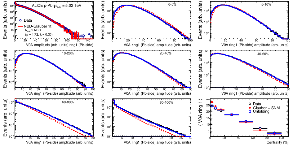
Within the Glauber-model, the consistency between measurements of in largely separated rapidity regions establishes their relation to centrality. To this end, we correlate the ZNA measurements to the amplitudes measured in the innermost ring of the VZERO-A detector (V0A ring1), since this ring covers the most forward rapidity in the Pb-going direction. The distributions () for centrality classes selected with ZNA () are obtained from the SNM-Glauber fit. These are convolved with the NBD obtained from the NBD-Glauber fit to the MB V0A ring1 distribution. Fig. 6 compares the distributions of V0A ring1 obtained from these convolutions to the ones measured in the same ZNA centrality classes. As expected, the distributions in the most peripheral events, where the SNM does not provide a reliable description of the data, are not well reproduced by the Glauber-MC convolution. In all other classes, the experimental distributions are well reproduced. The deviations are consistent with the ones between (see Table 3) and (see Table 7) assuming that the target-going charged-particle multiplicity measured in V0A ring1 is proportional to the number of wounded target nucleons.
In addition, Fig. 6 shows the results of an unfolding procedure. For each V0A ring1 distribution selected by a ZNA centrality class, we find the distribution that, convolved with the , fits the data, i.e. the parameters of the fit are the relative contributions of each bin. The unfolded distributions (shown in blue) agree well with the data for all centrality bins, apart from a small discrepancy in the 80-100% distribution at low amplitude, which is affected by trigger and event selection efficiency, however. The distribution which results from the sum of the unfolded distributions of all centrality bins agree well with the one from Glauber-MC. The existence of distributions that folded with NBD agree with measured signal distributions is a necessary condition for ZNA to behave as an unbiased centrality selection. In contrast, it is worth noting that a centrality selection based on central multiplicity, as CL1, has no such solution; i.e. no such good agreement can be found when the V0A ring1 distributions are selected by ordering the events according to CL1. The biases related to centrality selection will be discussed in the next section. The assumption that the ZNA selection is bias free will be used in Sec. 6 as an ansatz for the hybrid method.
5 Discussion of potential biases on centrality
5.1 Multiplicity Bias
Section 3.1 describes the NBD-Glauber fitting procedure used to determine the collision geometry in terms of and , for each centrality class. The NBD is used to account for multiplicity fluctuations at fixed . In contrast to Pb–Pb collisions, for p–Pb collisions these multiplicity fluctuations are sizeable compared to the width of the distribution, as illustrated in Fig. 7. For large fluctuations, a centrality classification of the events based on multiplicity may select a sample of nucleon-nucleon collisions which is biased compared to a sample defined by cuts on the impact parameter .


This selection bias, which occurs for any system with large relative statistical fluctuations in particle multiplicity per nucleon-nucleon collision, can be quantified using the Glauber fit itself. The left panel of Fig. 8 shows the ratio between the average multiplicity per average participant and the average multiplicity of the NBD as a function of centrality. In Pb–Pb collisions, where the width of the plateau of the distribution is large with respect to multiplicity fluctuations, the ratio deviates from unity only for the most peripheral collisions. As expected, in p–Pb collisions the ratio differs from unity for all centralities with large deviations for the most central and most peripheral collisions; the most central (peripheral) collisions have on average much higher (lower) multiplicity per participant. When selecting event classes using impact parameter intervals, there is no deviation from unity, as expected. The right panel of Fig. 8 shows for each centrality estimator the relative width of the NBD distribution (. As expected, the estimators with the largest bias on the multiplicity per participant correspond to those with the largest relative width.


It is instructive for the further discussion to consider the clan model [53], which is the standard physical explanation of the NBD distribution in the context of particle production in pp collisions. In this model particle sources, called ancestors, are produced independently according to a Poisson distribution with mean value, . Each ancestor can produce on average particles, e.g. by decay and fragmentation, and a clan contains all particles that stem from the same ancestor. Hence, the bias observed above also corresponds to a biased number of clans, which are sources of particle production. Analogously, in all recent Monte Carlo generators a large part of the multiplicity fluctuations is indeed due to the fluctuations of the number of particle sources, i.e. multiple semi-hard () parton-parton scatterings (MPI).
As an example, the HIJING generator accounts for fluctuations of the number of MPI per NN interaction via an NN overlap function , where is the NN impact parameter, i.e. the impact parameter between the proton and each wounded nucleon of the Pb-nucleus. The probability for inelastic NN collisions is given as one minus the probability to have no interaction:
| (6) |
where is the geometrical soft cross-section of 57 mb [29] related to the proton size and the energy dependent pQCD cross-section for parton scatterings. Further, as in the clan model, there is a Poissonian probability
| (7) |
for multiple hard collisions with an average number determined by :
| (8) |
Hence, the biases on the multiplicity discussed above correspond to a bias on the number of hard scatterings () and in the event. The latter correlates fluctuations over large rapidity ranges (long range correlations). As a consequence, for peripheral (central) collisions we expect a lower (higher) than average number of hard scatterings per binary collision, corresponding to a nuclear modification factor less than one (greater than one).


In general, the number of binary pN collisions, , is used to scale the reference pp yields and obtain the nuclear modification factor, used to quantify nuclear matter effects. However, for centrality classes based on multiplicity, owing to the bias induced by such selection, hard processes do not simply scale with but rather with an effective number of collisions, obtained by scaling the by the number of hard scatterings per pN collision: . As discussed in the HIJING example above, the number of hard scatterings per pN collision is simulated in Monte Carlo models. In this specific MC, even without bias, the total number of hard scatterings deviates from simple -scaling due to energy conservation at high . Instead, with the objective to study a baseline corresponding to an incoherent and unconstrained superposition of nucleon-nucleon collisions, the PYTHIA [54] event generator has been coupled to the p–Pb MC Glauber calculation. For each MC Glauber event PYTHIA is used to generate independent pp collisions. In the following we refer to this model as G-PYTHIA. In this model, the number of hard scatterings per pN collision shows a strong deviation from scaling which is illustrated in Fig. 10 and resembles the bias observed in Fig. 8.

5.2 Jet-veto bias
Additional kinematic biases exist for events containing high- particles. These particles arise from the fragmentation of partons produced in parton-parton scattering with large momentum transfer. Their contribution to the overall multiplicity rises with parton energy and, thus, can introduce a trivial correlation between the centrality estimator and the presence of a high- particle in the event. In particular, for very peripheral collisions, the multiplicity range that governs the centrality for the bulk of soft collisions can represent an effective veto on hard processes, leading to a . This bias is illustrated in Fig. 10. It shows a multiplicity distribution which is used as centrality estimators in p–Pb collisions, compared to the same distribution in pp collisions at = 7 TeV. The dashed lines mark the 80% and the 60% percentile of the p–Pb cross-section. The fraction of the pp cross-section selected with the 80-100% (60-100%) p–Pb multiplicity cut is 0.8 (0.97). The 80% cut in p–Pb is smaller than the multiplicity range covered in pp, therefore resulting in an effective veto on the large multiplicity events produced by hard processes.
5.3 Geometric bias
The dependence of particle production postulated in section 5.1 leads to a purely geometrical, centrality estimator independent bias for peripheral p–Pb collisions [55]. As illustrated in Fig. 11, the mean impact parameter between two nucleons (), calculated from a Monte Carlo Glauber simulation, is almost constant for central collisions, but rises significantly for . This reduces the average number of MPIs for most peripheral events, enhancing the effect of the bias leading to a nuclear modification factor less than (greater than) one for peripheral (central) collisions.
In summary, based on simplified models we have identified three different possible biases that are expected to lead to deviations from unity at high of the nuclear modification factors in peripheral and central collisions. As will be discussed and studied in the following sections, the effect decreases with increasing rapidity separation between the measurement and the centrality estimator.
For the estimators we used, the main biases are:
- 1.
CL1: strong bias due to the full overlap with tracking region. Additional bias from the “jet veto effect”, as jets contribute to the multiplicity and shift events to higher centralities (-dependent) ;
- 2.
V0M: reduced bias since the VZERO hodoscopes are outside the tracking region;
- 3.
V0A: reduced bias because of the enhanced contribution from the Pb fragmentation region;
- 4.
ZNA: no bias expected.
In addition, independent of the centrality estimator, there is a geometrical bias for peripheral collisions (see Sec.5.3).
6 The Hybrid Method
6.1 Basis and assumptions of the method
The hybrid method presented in the following section aims to provide an unbiased centrality estimator and relies on two main assumptions. The first is to assume that an event selection based on ZN does not introduce any bias on the bulk at mid-rapidity and on high- particle production. This assumptions is based on the results from the unfolding procedure presented in Sec.4 and the full acceptance of ZN for neutrons emitted from the Pb nucleus, also discussd in Sec.4. In addition consistent results where obtained with proton calorimeter ZP, in the region of its full acceptance. Therefore we do not expect a significant bias from the ZN selection and herein this is taken as ansatz. This selection was also used in the method proposed in Sec.4, however the determination provded by the SNM-Glauber model is model-dependent. In contrast, in the hybrid method, the determination is based -as an ansatz- on a particular scaling for particle multiplicity (the second assumption), e.g. we assume that the charged-particle multiplicity measured at mid-rapidity scales with the number of participants.
To obtain more insight into the particle production mechanisms, we study the correlation of various pairs of observables that, in ZN-centrality classes, are expected to scale linearly with or . One of these observables is the charged-particle density in , measured with the SPD. The charged particle pseudorapidity density is obtained from the measured distribution of tracklets, formed using the position of the primary vertex and two hits, one on each SPD layer [24]. At larger pseudorapidities, where a direct multiplicity measurement is not available, we study the raw signals of the four rings of VZERO-A and VZERO-C detectors separately. We exploit both beam configurations, p–Pb and Pb–p in order to cover the widest possible rapidity range. To take into account the impact of secondary particles, the pseudorapidity coverage of the VZERO detector rings with respect to the primary charged particles was calculated with a full detector simulation based on DPMJET [52, 51] and it is given in Table 6 in the centre-of-mass system (cms), which moves with a rapidity of in the direction of the proton beam (see Sec. 2).
| Ring | (p–Pb) | (Pb–p) |
|---|---|---|
| VZERO-A ring 1 | -5.39 | 4.45 |
| VZERO-A ring 2 | -4.80 | 3.87 |
| VZERO-A ring 3 | -4.28 | 3.35 |
| VZERO-A ring 4 | -3.82 | 2.89 |
| VZERO-C ring 1 | 3.34 | -4.26 |
| VZERO-C ring 2 | 2.82 | -3.74 |
| VZERO-C ring 3 | 2.33 | -3.25 |
| VZERO-C ring 4 | 1.86 | -2.78 |
The information about charged particle multiplicity, dominated by soft particles, is complemented with observables from hard processes which are expected to scale with the number of binary collisions, such as the yield of high- (10 < < 20 GeV/) particles measured at mid-rapidity ().
In order to compare these observables on the same scale and also, at first order, to neglect detector efficiency and acceptance effects, we use so called normalized signals . These are obtained dividing , i.e. the mean value of , number of raw SPD tracklets or raw VZERO signal in a given ZN-centrality class , by the corresponding mean values in minimum bias collisions.
Figure 12 shows, for bins in ZN centrality, the correlation between a few selected normalized signals and the normalized charged-particle density averaged over . The statistical uncertainty is negligible, while the systematic uncertainties largely cancel in the ratio to the MB signals.


One can note that the correlation exhibits a clear dependence on the pseudorapidity of the normalized signal. The slope of the normalized signals with diminishes towards the proton direction (C-side in p–Pb collisions). For example, in the innermost ring of the VZERO-C detector the signal amplitude range is about a factor three, while for the innermost ring of the VZERO-A detectors it is about twice as large.
In the Wounded Nucleon Model [18], the total number of participants is expressed in terms of target and projectile participants. The charged particle density at mid-rapidity is thus proportional to , whereas at higher rapidities the model predicts a dependence on a linear combination of the number of target and projectile participants with coefficients which depend on the rapidity. Close to Pb-rapidity a linear wounded target nucleon scaling ( = - 1) is expected.
In order to further understand the relative trends of the observables in Fig. 12 and to relate them with geometrical quantities, such as , one can adopt the Wounded Nucleon Model and make the assumption that in is proportional to . In this case, the other observables can be related to , assuming linear or power-law dependence. The linear dependence can be parameterized with , where is a free parameter. Then the normalized signals can be expressed with and one obtains the following linear relation:
| (9) |
where = 7.9 is the average number of participating nucleons in minimum bias collisions. The relation is used to find for each observable by a fit to the data. Analogously, we can also fit a power-law function as:
| (10) | |||||
where the are the width of the centrality classes and is a fit parameter. Since we made the assumption that in is proportional to , obtained from Eq. 10 equivalently quantifies the deviations from a perfect () scaling. As can be seen from the lower panels of Fig. 12 the power-law fit describes the data better, especially for the observables located further away from mid-rapidity. This also means that the linear dependence assumed in Eq.9 can only be valid approximately.


Fig. 13 shows the results of the fits in Eq. 9 and 10 as a function of of the measured observables. The figure displays data collected in both p–Pb and Pb–p beam configurations. Since the Pb–p data were taken at high-luminosity (reaching 200 kHz, roughly corresponding to a luminosity of 10), the results are affected by interaction pile-up (probability per bunch crossing between 3.8-4.3%). In order to reduce the effect of the pile-up and to treat p–Pb and Pb–p data consistently, we excluded the 0-5% centrality class from the fits. Furthermore, in order to take into account the remaining distortions in the 5-100% classes, the Pb–p data were corrected using the results for the tracklets (also shown in Fig. 13) in a small -region, (), where is nearly identical for p–Pb and Pb–p configurations. Typically the absolute correction is 0.05 and 0.01 for the and parameters, respectively.
The results presented in Fig. 13 indicate a smooth and continuous change of the scaling behaviour for charged particle production with pseudorapidity. It is worth noting that at large negative pseudorapidity (Pb-going direction) the values of the parameters and reach those obtained for charged-particle production at high- . In contrast, the parameter values are much lower in the proton-going direction. Our data are overlaid with the corresponding fit parameters derived from PHOBOS charged-particle multiplicity measurements in d–Au collisions at = 200 GeV [21]. The normalized charged-particle multiplicity in each pseudorapidity bin is fit against using Eq. 9 and 10. The results obtained in this way are then adjusted by scaling the x-axis () by the ratio of the beam rapidities in p–Pb at = 5.02 TeV and d–Au collisions at = 200 GeV. The comparison between PHOBOS and our data shows a good agreement over a wide range, with some deviations at large negative pseudorapidity. In particular, the region covered by the innermost ring of the VZERO-A detector corresponds to the target fragmentation region where extended longitudinal scaling was observed at RHIC [21]. The minimum bias and are obtained by PHOBOS relying on a tuned HIJING-based Monte Carlo simulation [21].
6.2 Calculation of
As discussed in the previous section, selecting the events using the ZN signal is expected to be free from bias on the bulk multiplicity or high- particle yields. In order to establish a relationship to the collision geometry, we exploit the findings from the correlation analysis described above and make use of observables that are expected to scale as a linear function of or .
Three sets of values are calculated, based on the following assumptions:
- 1.
: the charged-particle multiplicity at mid-rapidity is proportional to the number of participants ();
- 2.
: the yield of charged high- particles at mid-rapidity is proportional to the number of binary NN collisions ();
- 3.
: the target-going charged-particle multiplicity is proportional to the number of wounded target nucleons ( = - 1 = ).
For the charged-particle multiplicity in the Pb-going side we use the signal from the innermost ring of the VZERO-A detector. We note that assumptions 1) and 2) are satisfied for minimum bias collisions, where we measured a value of consistent with that in inelastic pp collisions (0.97 0.08) [24] and an integrated (10 < < 20 GeV/) = 0.995 0.010 (stat.) 0.090 (syst.) (see Sec. 7).
Therefore, in order to obtain the average number of binary NN collisions in each centrality interval, the minimum bias value of = 7.9, is scaled using the ratio of the multiplicity at mid-rapidity:
| (11) | |||||
| (12) |
In a similar way the minimum bias value of = 6.9 is scaled using the ratio of the yield of high- particles at mid-rapidity to obtain :
| (13) |
where stands for the charged-particle yields with GeV/. Alternatively, one can use the Pb-side multiplicity to obtain
| (14) |
where stands for the raw signal of the innermost ring of VZERO-A. The obtained values of in ZN-centrality classes are listed in Table 7 and shown in Fig. 14.
| Centrality | |||
|---|---|---|---|
| 0 - 5 | 12.2 | 12.5 | 13.3 |
| 5 - 10 | 11.6 | 12.1 | 12.3 |
| 10 - 20 | 11.0 | 11.3 | 11.4 |
| 20 - 40 | 9.56 | 9.73 | 9.60 |
| 40 - 60 | 7.08 | 6.81 | 6.74 |
| 60 - 80 | 4.30 | 4.05 | 4.00 |
| 80 - 100 | 2.11 | 2.03 | 2.06 |


The systematic uncertainty is given by the 8% uncertainty on the (or the 3.4% uncertainty on the ) listed in Table 3. We assign no uncertainty to the assumptions made for particle scaling. The differences between the three sets of values do not exceed 9% in all centrality classes. This confirms the consistency of the assumptions used, but it does not prove that any (or all) of the assumptions are valid. We note that these values, in particular , agree within 18% with those calculated with the SNM (see Fig. 2 and Table 3), except for the most peripheral reactions, where the SNM is inaccurate.
In addition, we plot in Fig. 15 the zero degree signal from neutral particles in the proton-going direction ZNC vs . We have excluded events without a signal in the ZNC, however the qualitative trend does not change when including those events. Over a wide range of centralities (10-100%) a linear anti-correlation is observed. This is consistent with a longitudinal energy transfer of the proton proportional to the number of binary collisions.
7 Results and implications for particle production
7.1 Charged Particle Density
The measurement of the centrality dependence of the particle multiplicity density allows a discrimination between models that describe the initial state of heavy ion collisions. In [24] we described the charged particle pseudorapidity density in minimum bias collisions. The same analysis was repeated, dividing the visible cross-section (see Sec.2) into event classes defined by the centrality estimators described above, and the values associated to each centrality interval were calculated using the methods discussed in Sec. 3, 4, 6.
The results of the charged particle multiplicity density as a function of the pseudorapidity are presented in Fig. 16 for different centrality intervals and different centrality estimators. The fully correlated systematic uncertainty, is given by the quadrature sum of the 2.2% minimum bias error detailed in [24], and an -dependent uncertainty from the vertex efficiency and the centrality selection.
In peripheral collisions (60-80% and 80-100%) the shape of the distribution is almost fully symmetric and resembles what is seen in proton-proton collisions. In more central collisions, the shape of becomes progressively more asymmetric, with an increasing excess of particles produced in the direction of the Pb beam compared to the proton-going direction.


The shape of the pseudorapidity density function is sensitive to details of particle production models. For example, it was found in [24] that in minimum bias reactions the dependence is described relatively well by HIJING [56] or DPMJET[52], with a gluon shadowing parameter tuned to describe experimental data at lower energy, whereas the saturation models [57, 58, 59] exhibit a steeper dependence than the data. We have quantified the centrality evolution of the pseudorapidity shape for the different centrality estimators by analyzing the density at mid-rapidity, and the asymmetry of particle yield between the proton and the Pb peak regions, as the ratio of at and , symmetrically around the centre of mass. This is shown in Fig. 17.

Figure 18 shows the integrated at mid-rapidity divided by the number of participants as a function of (left) or as a function of (right) for various centrality estimators. The systematic uncertainty is smaller than the marker size. For the V0A centrality estimator, in addition to the from the standard Glauber calculation, the results obtained with the implementation of Glauber-Gribov model (with ) are also shown. For CL1, V0M, and V0A, the charged particle density at mid-rapidity has as steeper than linear increase, as a consequence of the strong multiplicity bias discussed in Sec. 5, which is strongest in CL1, where the overlap with the tracking region is maximum. This trend is not seen in the case of the Glauber-Gribov model, which shows a relatively constant behaviour for the integrated yield divided by the number of participant pairs, with the exception of the most peripheral point.
For ZNA, there is a clear sign of saturation above , as the values are closer to each other. Most probably, this is due to the saturation of forward neutron emission. We note that none of these curves point towards the pp data point. This suggests that the geometry bias, present in peripheral collisions, together with the multiplicity bias for CL1, V0M and V0A, has a large effect on this centrality class.
In contrast, the results obtained with the hybrid method, where the and the give very similar trends, show, within , scaling with , which naturally reaches the pp point, well within the quoted uncertainty of 8% on the values. In addition, they show that the range in covered with an unbiased centrality selection is more limited than what is obtained using estimators based on particle multiplicity. The latter do not select on the collision geometry but rather on the final products of the collision. This effect is emphasized in the right plot, which shows the same quantity divided by as a function of . Here the limited range in reached with the ZNA selection is clearly visible. This indicates the sensitivity of the -scaling behaviour to the Glauber modelling, as well as the importance of the multiplicity fluctuations.


7.2 Nuclear modification factors
As discussed in section 5, the various centrality estimators induce a bias on the nuclear modification factor depending on the rapidity range they cover. In contrast to minimum bias collisions, where is fixed by the ratio of the pN and p–Pb cross-sections, in general, for a given centrality class cannot be used to scale the pp cross-section, or to calculate centrality-dependent nuclear modification factors. For a centrality selected event sample, we therefore define as
| (15) |
for a given centrality percentile according to a particular centrality estimator. In our notation we distinguish from because the former is influenced by potential biases from the centrality estimator which are not related to nuclear effects. Hence, can be different from unity even in the absence of nuclear effects.
The distribution of primary charged particles in minimum bias collisions is given in [60]. The charged particle spectra are reconstructed with the two main ALICE tracking detectors, the Inner Tracking System and the Time Projection Chamber, and are corrected for the detector and reconstruction efficiency using a Monte Carlo simulation based on the DPMJET event generator [52]. The systematic uncertainties on corrections are estimated via a comparison to a Monte Carlo simulation using the HIJING event generator [29], while the resolution is estimated from the space-point residuals to the track fit and verified with data. The total systematic uncertainty ranges between 3.4% and 6.7% in the measured range, 0.15-50 GeV/, with a negligible dependence. The nuclear modification factor is calculated by dividing the data by the reference pp spectrum scaled by . The reference pp spectrum is obtained at low ( 5 GeV/) by interpolating the data measured at = 2.76 and 7 TeV, and at high ( 5 GeV/) by scaling the measurements at = 7 TeV with the ratio of spectra calculated with NLO pQCD at = 5.02 and 7 TeV [61]. The systematic uncertainty, given by the largest of the relative systematic uncertainties of the spectrum at 2.76 or 7 TeV at low-, and assigned from the relative difference between the NLO-scaled spectrum for different scales and the difference between the interpolated and the NLO-scaled data at high-, ranges from 6.8% to 8.2%. For MB collisions the nuclear modification factor is consistent with unity for above 6 GeV/c.
The same analysis was repeated dividing the visible cross-section (see Sec.2) in event classes defined by the centrality estimators described above, and the were calculated using the values of listed in Tables 3 and 7, for each given estimator. Figure 19 shows the for different centrality estimators and different centrality classes. The uncertainties of the p–Pb and pp spectra are added in quadrature, separately, for the statistical and systematic uncertainties. The systematic uncertainty on the spectra is only shown for the V0A 0-5% centrality bin and is the same for all others, since all the corrections are independent of centrality. The total systematic uncertainty on the normalization, given by the quadratic sum of the uncertainty on the normalization of the pp data and the normalization of the p–Pb data, amounts to 6.0% and is shown as a gray box around unity. The systematic uncertainty on is shown as a light blue box around unity. For simplicity, we draw only the uncertainty for the minimum bias value .


As expected, for CL1, V0M and V0A, strongly deviates from unity at high in all centrality classes, with values well above unity for central collisions and below unity for peripheral collisions. However the spread between centrality classes reduces with increasing rapidity gap between the range used for the centrality estimator and that used for the measurement. There is a clear indication of the jet-veto bias in the most peripheral CL1 class, where has a significant negative slope ( 5 GeV/) since the jet contribution to the total multiplicity increases with . This jet-veto bias diminishes for V0M, and is absent for V0A, where for peripheral collisions, indicating that the multiplicity bias is still present.
In order to study the centrality determination biases further, the spectra are compared to the G-PYTHIA spectra. The event centrality is obtained from the charged particle multiplicity in the rapidity region covered by each estimator in the same way as in data, and is directly obtained from the Monte Carlo. The calculation is shown as lines in Fig. 19. With this approach, the general trend at high is reasonably well described for all centrality classes, particularly for CL1. This suggests that particle production at high in p–Pb collisions indeed can be approximated by an an incoherent superposition of pp collisions. The agreement, however, is not as good for the V0A and V0M estimators, since the model is not adequate for forward particle production, particularly in the target fragmentation region. G-PYTHIA also reproduces the jet-veto bias, as indicated by the good agreement of the dependence in the low and intermediate region in the most peripheral CL1 collisions.
However, for central collisions, the values show a significant enhancement at intermediate 3 GeV/ (called the Cronin effect, a nuclear modification factor above unity at intermediate , observed at lower energies in p–A collisions [62, 63, 25, 64]), which increases with centrality independently of the estimator used. The enhancement in the intermediate region is about 15%, and the differences in the height of the peak among centrality estimators are small with respect to the absolute increases of the p–Pb yields. The enhancement is not reproduced by our model of incoherent superposition of pp collisions. In contrast, in the low region, below the Cronin peak, the yield is overestimated by the model. This overestimate at low is expected because this region is dominated by soft processes and therefore is not expected to scale with . On the other hand, the intermediate region is expected to be dominated by hard scatterings and should scale with in the absence of nuclear effects. From this we can conclude that the Cronin enhancement observed is due to nuclear modification effects, as observed in other measurements [10, 11, 12, 13], as well as in the minimum bias [2].
The bottom right plot of Fig. 19 shows the for the ZNA centrality selection. The classes selected by the ZNA present spectra much more similar to each other than the other estimators, as expected in the absence of a multiplicity bias. The height of the Cronin peak relative to the yield at high- is larger with the V0A selection, which may be seen as a sign of a remaining small bias in V0A, expected from the G-PYTHIA calculations. However, for peripheral collisions (60-80% and 80-100%), the absolute values of the spectra at high indicate the presence of a bias on in the ZNA measurement. This is not due to the event selection, but is due to the inaccurate estimate of values for peripheral events, where a small, absolute uncertainty results in a large relative deviation in the calculation.


As discussed in Sec. 6, the hybrid method uses centrality classes selected with ZNA and values determined with assumptions on particle production. Fig. 20 shows the resulting values, on the left and on the right panel. Here it is important to note that the ratios in the lower right panel in Fig. 19, and both panels in Fig. 20 have the same shape by construction, and only differ due to the scaling () of the reference. The small differences among the values (Table 7) are reflected in consistent , which also remain consistent with unity at high- for all centrality classes. This confirms the absence of initial state effects, already observed for minimum bias collisions. The Cronin enhancement, which has already been noted in minimum bias collisions, is observed to be stronger in central collisions and nearly absent in peripheral collisions. The enhancement is also weaker at 5.02 TeV compared to 200 GeV [62]. The geometry bias, described in Sec.5.3, is still present and uncorrected, even with this method. Its effect is limited to only peripheral classes, resulting in for 80-100%.
Fig. 21 shows the mean at high momentum as a function of centrality for the various centrality estimators. The centrality dependence of extracted from multiplicity distributions is shown on the left. It is reminiscent of the multiplicity bias, and reproduced by the G-PYTHIA calculation (lines in the figure). The mean changes less with increasing rapidity gap between the centrality estimator and the region where the measurement is performed, as expected from the multiplicity bias. Instead, the extracted with the hybrid model (Fig. 21 right) is consistent with unity and the results from the two assumptions used for the calculation are in agreement.
To compare the impact of the multiplicity bias from the different estimators on the nuclear modification factors, the ratio of the spectra in pp and p–Pb in different momentum ranges () is divided by the ratio of charged particle density at mid-rapidity in pp and p–Pb () and it is plotted as a function of () in Fig. 22. Left and middle panels show the yield at high- (10-20 GeV/) and around the Cronin peak (3 GeV/), respectively. Figure 22 clearly shows the shape bias on particle spectra. Even for the same average event activity at mid-rapidity (corresponding to the same point on the x-axis ), the spectra show a small but significant dependence on the centrality estimator. This is visible as a different relative number of particles () in the intermediate (3 GeV/) or in the high- (10-20 GeV/) region. Also the height of the Cronin peak relative to the high- yield depends on the centrality estimator. This is shown in the right panel of Fig. 22, which plots the double ratio of the p–Pb to pp yields at 3 GeV/ and in 10-20 GeV/ (). Since, for CL1, is not constant at high we plot also the ratio to the value calculated with G-PYTHIA at 3 GeV/. The Cronin peak is clearly visible for the V0M and CL1 (with respect to G-PYTHIA) selection, and very pronounced for the V0A selection. As previously noted, the ZNA selection shows a similar trend and similar value as V0A, when restricted to the range common to both estimators. However the differences are still significant, and the common range is still rather small. In particular, the height of the Cronin peak is larger with ZNA than with V0A in the common range, which may be seen as a sign of a remaining small bias in V0A, confirming what is observed by G-PYTHIA calculations.
The study of the correlation between observables measured in such different parts of phase space has shown that it is possible to select similar event classes using estimators that are causally disconnected after the interaction. This is very important because this suggests that any such correlation can only arise from the initial geometry of the collision.

8 Summary
In summary, we have studied the centrality dependence of charged particle production, with measurements that comprise the charged particle pseudorapidity density and the nuclear modification factor. The methods to determine centrality in p–A collisions using multiplicity measurements or zero-degree energy have been presented in detail. The former induce a bias on the hardness of the pN collisions that can be quantified by the number of hard scatterings per pN collision. Low (high) multiplicity p–Pb corresponds to lower (higher) than average number of hard scatterings. For observables based on centrality estimates from multiplicity, nuclear effects should be calculated, including this bias when comparing to an incoherent superposition of pN collisions.
In contrast, the energy deposited at zero degrees by slow nucleons in the ZDC is expected to be insensitive to a multiplicity bias. Under this assumption, but in the absence of a model which properly relates the ZDC energy to the number of collisions, these are calculated assuming multiplicity scaling laws in the given kinematic ranges. In particular, we assume that the multiplicity at mid-rapidity is proportional to , that multiplicity in the target-going direction is proportional to the number of wounded target nucleons, or that the yield of high- particles is proportional to . The equivalence of these assumptions has been shown and discussed. Therefore, under these assumptions, we find i) that nuclear modification factors are consistent with unity above 8 GeV/c, with no centrality dependence; ii) that the multiplicity of charged particles at mid-rapidity scales linearly with the total number of participants; iii) and that the longitudinal features of p–Pb collisions at TeV, as reflected by the centrality dependence of the pseudorapidity distributions of charged particles, are very similar to those seen in d–Au collisions at RHIC energies. The latter were interpreted in support of extended longitudinal scaling in the fragmentation regions. These results represent valuable input for the study of the event activity dependence of hard probes in p-Pb collision and, hence, help to establish baselines for the interpretation of the Pb-Pb data.
Acknowledgements
The ALICE Collaboration would like to thank all its engineers and technicians for their invaluable contributions to the construction of the experiment and the CERN accelerator teams for the outstanding performance of the LHC complex. The ALICE Collaboration gratefully acknowledges the resources and support provided by all Grid centres and the Worldwide LHC Computing Grid (WLCG) collaboration. The ALICE Collaboration acknowledges the following funding agencies for their support in building and running the ALICE detector: State Committee of Science, World Federation of Scientists (WFS) and Swiss Fonds Kidagan, Armenia, Conselho Nacional de Desenvolvimento Científico e Tecnológico (CNPq), Financiadora de Estudos e Projetos (FINEP), Fundação de Amparo à Pesquisa do Estado de São Paulo (FAPESP); National Natural Science Foundation of China (NSFC), the Chinese Ministry of Education (CMOE) and the Ministry of Science and Technology of China (MSTC); Ministry of Education and Youth of the Czech Republic; Danish Natural Science Research Council, the Carlsberg Foundation and the Danish National Research Foundation; The European Research Council under the European Community’s Seventh Framework Programme; Helsinki Institute of Physics and the Academy of Finland; French CNRS-IN2P3, the ‘Region Pays de Loire’, ‘Region Alsace’, ‘Region Auvergne’ and CEA, France; German Bundesministerium fur Bildung, Wissenschaft, Forschung und Technologie (BMBF) and the Helmholtz Association; General Secretariat for Research and Technology, Ministry of Development, Greece; Hungarian Orszagos Tudomanyos Kutatasi Alappgrammok (OTKA) and National Office for Research and Technology (NKTH); Department of Atomic Energy and Department of Science and Technology of the Government of India; Istituto Nazionale di Fisica Nucleare (INFN) and Centro Fermi - Museo Storico della Fisica e Centro Studi e Ricerche "Enrico Fermi", Italy; MEXT Grant-in-Aid for Specially Promoted Research, Japan; Joint Institute for Nuclear Research, Dubna; National Research Foundation of Korea (NRF); Consejo Nacional de Cienca y Tecnologia (CONACYT), Direccion General de Asuntos del Personal Academico(DGAPA), México, :Amerique Latine Formation academique – European Commission(ALFA-EC) and the EPLANET Program (European Particle Physics Latin American Network) Stichting voor Fundamenteel Onderzoek der Materie (FOM) and the Nederlandse Organisatie voor Wetenschappelijk Onderzoek (NWO), Netherlands; Research Council of Norway (NFR); Polish Ministry of Science and Higher Education; National Science Centre, Poland; Ministry of National Education/Institute for Atomic Physics and Consiliul Naţional al Cercetării Ştiinţifice - Executive Agency for Higher Education Research Development and Innovation Funding (CNCS-UEFISCDI) - Romania; Ministry of Education and Science of Russian Federation, Russian Academy of Sciences, Russian Federal Agency of Atomic Energy, Russian Federal Agency for Science and Innovations and The Russian Foundation for Basic Research; Ministry of Education of Slovakia; Department of Science and Technology, South Africa; Centro de Investigaciones Energeticas, Medioambientales y Tecnologicas (CIEMAT), E-Infrastructure shared between Europe and Latin America (EELA), Ministerio de Economía y Competitividad (MINECO) of Spain, Xunta de Galicia (Consellería de Educación), Centro de Aplicaciones Tecnológicas y Desarrollo Nuclear (CEADEN), Cubaenergía, Cuba, and IAEA (International Atomic Energy Agency); Swedish Research Council (VR) and Knut Alice Wallenberg Foundation (KAW); Ukraine Ministry of Education and Science; United Kingdom Science and Technology Facilities Council (STFC); The United States Department of Energy, the United States National Science Foundation, the State of Texas, and the State of Ohio; Ministry of Science, Education and Sports of Croatia and Unity through Knowledge Fund, Croatia. Council of Scientific and Industrial Research (CSIR), New Delhi, India
References
- [1] C. Salgado, J. Alvarez-Muniz, F. Arleo, N. Armesto, M. Botje, et al., “Proton-Nucleus Collisions at the LHC: Scientific Opportunities and Requirements,” J.Phys.G G39 (2012) 015010, arXiv:1105.3919 [hep-ph].
- [2] ALICE Collaboration, B. Abelev et al., “Transverse momentum distribution and nuclear modification factor of charged particles in p–pb collisions at 5.02 tev,” Phys. Rev. Lett. 110 (Feb, 2013) 082302. http://link.aps.org/doi/10.1103/PhysRevLett.110.082302.
- [3] CMS Collaboration, S. Chatrchyan et al., “Measurement of isolated photon production in and PbPb collisions at TeV,” Phys.Lett. B710 (2012) 256–277, arXiv:1201.3093 [nucl-ex].
- [4] ATLAS Collaboration, G. Aad et al., “Measurement of boson Production in Pb+Pb Collisions at TeV with the ATLAS Detector,” Phys.Rev.Lett. 110 (2013) 022301, arXiv:1210.6486 [hep-ex].
- [5] CMS Collaboration, S. Chatrchyan et al., “Study of Z boson production in PbPb collisions at nucleon-nucleon centre of mass energy = 2.76 TeV,” Phys.Rev.Lett. 106 (2011) 212301, arXiv:1102.5435 [nucl-ex].
- [6] ALICE Collaboration, K. Aamodt et al., “Suppression of charged particle production at large transverse momentum in central pb–pb collisions at,” Physics Letters B 696 no. 1–2, (2011) 30 – 39. http://www.sciencedirect.com/science/article/pii/S0370269310013973.
- [7] ALICE Collaboration, B. Abelev et al., “Measurement of charged jet suppression in Pb-Pb collisions at = 2.76 TeV,” JHEP 1403 (2014) 013, arXiv:1311.0633 [nucl-ex].
- [8] ALICE Collaboration, B. Abelev et al., “Suppression of high transverse momentum d mesons in central pb-pb collisions at ,” Journal of High Energy Physics 112 no. 9, (2012) 1–37.
- [9] ALICE Collaboration, B. B. Abelev et al., “ production and nuclear effects in p-Pb collisions at = 5.02 TeV,” JHEP 1402 (2014) 073, arXiv:1308.6726 [nucl-ex].
- [10] ALICE Collaboration, B. Abelev et al., “Long-range angular correlations on the near and away side in -Pb collisions at TeV,” Phys.Lett. B719 (2013) 29–41, arXiv:1212.2001 [nucl-ex].
- [11] ALICE Collaboration, B. Abelev et al., “Multiplicity dependence of the average transverse momentum in pp, p-Pb, and Pb-Pb collisions at the LHC,” Phys.Lett. B727 (2013) 371–380, arXiv:1307.1094 [nucl-ex].
- [12] ALICE Collaboration, B. Abelev et al., “Multiplicity Dependence of Pion, Kaon, Proton and Lambda Production in p-Pb Collisions at = 5.02 TeV,” Phys.Lett. B728 (2014) 25–38, arXiv:1307.6796 [nucl-ex].
- [13] ALICE Collaboration, B. Abelev et al., “Long-range angular correlations of pi, K and p in p–Pb collisions at TeV,” Phys.Lett. B726 (2013) 164–177, arXiv:1307.3237 [nucl-ex].
- [14] K. Dusling and R. Venugopalan, “Comparison of the color glass condensate to dihadron correlations in proton-proton and proton-nucleus collisions,” Phys.Rev. D87 no. 9, (2013) 094034, arXiv:1302.7018 [hep-ph].
- [15] P. Bozek, “Collective flow in p-Pb and d-Pd collisions at TeV energies,” Phys.Rev. C85 (2012) 014911, arXiv:1112.0915 [hep-ph].
- [16] M. Miller, K. Reygers, S. J. Sanders, and P. Steinberg, “Glauber modeling in high energy nuclear collisions,” Ann. Rev. Nucl. Part. Sci. 57 (2007) 205–243, arXiv:nucl-ex/0701025.
- [17] B. Bialas, A. and W. Czyz, “Multiplicity distributions in nucleus-nucleus collisions at high energies,” Nucl.Phys. B111 (1976) 461.
- [18] A. Bialas and A. Bzdak, “Wounded quarks and diquarks in high energy collisions,” Phys.Rev. C77 (2008) 034908, arXiv:0707.3720 [hep-ph].
- [19] H. Pi, “An Event generator for interactions between hadrons and nuclei: FRITIOF version 7.0,” Comput.Phys.Commun. 71 (1992) 173–192.
- [20] E178 Collaboration, J. Elias et al., “An experimental study of multiparticle production in hadron - nucleus interactions at high-energy,” Phys.Rev. D22 (1080) 13.
- [21] PHOBOS Collaboration, B. Back et al., “Scaling of charged particle production in d + Au collisions at s(NN)**(1/2) = 200-GeV,” Phys.Rev. C72 (2005) 031901, arXiv:nucl-ex/0409021 [nucl-ex].
- [22] PHENIX Collaboration, A. Adare et al., “Centrality categorization for in high-energy collisions,” arXiv:1310.4793 [nucl-ex].
- [23] STAR Collaboration, J. Adams et al., “Evidence from d + Au measurements for final state suppression of high p(T) hadrons in Au+Au collisions at RHIC,” Phys.Rev.Lett. 91 (2003) 072304, arXiv:nucl-ex/0306024 [nucl-ex].
- [24] ALICE Collaboration, B. Abelev et al., “Pseudorapidity density of charged particles in p+pb collisions at 5.02tev,” Phys. Rev. Lett. 110 (Jan, 2013) 032301. http://link.aps.org/doi/10.1103/PhysRevLett.110.032301.
- [25] STAR Collaboration, J. et al., “Pion, kaon, proton and anti-proton transverse momentum distributions from and collisions at,” Physics Letters B 616 no. 1–2, (2005) 8 – 16. http://www.sciencedirect.com/science/article/pii/S0370269305005381.
- [26] F. Sikler, “Centrality control of hadron nucleus interactions by detection of slow nucleons,” arXiv:hep-ph/0304065 [hep-ph].
- [27] ALICE Collaboration, B. Alessandro et al., “"physics performance report ii",” PPR vol. II: J. Phys. G32 no. G32, (2006) 1295.
- [28] V. Gribov, “Glauber corrections and the interaction between high-energy hadrons and nuclei,” Sov. Phys. JETP 29 (1969) 483–487.
- [29] X.-N. Wang and M. Gyulassy, “Hijing: A monte carlo model for multiple jet production in pp, pa, and aa collisions,” Phys. Rev. D 44 (1991) 3501.
- [30] ALICE Collaboration, K. Aamodt et al., “The alice experiment at the cern lhc,” J. Instrum. 3 (2008) S08002.
- [31] ALICE Collaboration, B. B. Abelev et al., “Performance of the ALICE Experiment at the CERN LHC,” Int.J.Mod.Phys. A29 (2014) 1430044, arXiv:1402.4476 [nucl-ex].
- [32] ALICE Collaboration, B. B. Abelev et al., “Measurement of visible cross sections in proton-lead collisions at sqrt(sNN) = 5.02 TeV in van der Meer scans with the ALICE detector,” arXiv:1405.1849 [nucl-ex].
- [33] R. Glauber, “Lectures in theoretical physics,” ed WE Brittin and LG Dunham 1 (1959) 315.
- [34] R. Glauber, “Cross sections in deuterium at high energies,” Phys. Rev. 100 (1955) 242.
- [35] R. Glauber, “Quantum optics and heavy ion physics,” Nucl. Phys. A 774 (2006) 3.
- [36] A. P. T.W. Ludlam and A. Shor, “Hijet. a monte carlo event generator for p–nucleus and nucleus–nucleus collisions,” BNL 37196 (1985) 373–381.
- [37] A. Shor and R. Longacre, “Effects of secondary interactions in proton-nucleus and nucleus-nucleus collisions using the hijet event generator,” Phys. Lett. B 218 (1989) 100.
- [38] ALICE Collaboration, B. Abelev et al., “Centrality determination of Pb-Pb collisions at = 2.76 TeV with ALICE,” Phys.Rev. C88 no. 4, (2013) 044909, arXiv:1301.4361 [nucl-ex].
- [39] H. De Vries, C. W. De Jager, and C. De Vries, “Nuclear charge and magnetization density distribution parameters from elastic electron scattering,” Atom. Data Nucl. Data Tabl. 36 (1987) 495–536.
- [40] Particle Data Group Collaboration, K. Nakamura et al., “Review of particle physics,” J. Phys. G37 (2010) 075021.
- [41] ALICE Collaboration, B. Abelev et al., “Measurement of inelastic, single- and double-diffraction cross sections in proton–proton collisions at the LHC with ALICE,” Eur.Phys.J. C73 (2013) 2456, arXiv:1208.4968 [hep-ex].
- [42] B. B. H. Heiselberg, G. Baym, L. Frankfurt, and M. Strikman, “Color transparency, color opacity and fluctuations in nuclear collisions,” Phys. Rev. Lett. 67 (1991) 2946–2949.
- [43] V. Guzey and M. Strikman, “Proton-nucleus scattering and cross section fluctuations at RHIC and LHC,” Phys.Lett. B633 (2006) 245–252, arXiv:hep-ph/0505088 [hep-ph].
- [44] M. Alvioli and M. Strikman, “Color fluctuation effects in proton-nucleus collisions,” Phys. Lett. B 722 (2013) 347–354.
- [45] ATLAS Collaboration, G. Aad et al., “Measurement of the charged particle multiplicity distribution in p+pb collision at tev with the atlas detector at lhc,” ATLAS-CONF-2013-096 (2013) .
- [46] C. Loizides, J. Nagle, and P. Steinberg, “Improved version of the PHOBOS Glauber Monte Carlo,” arXiv:1408.2549 [nucl-ex].
- [47] E910 Collaboration, I. Chemakin et al., “Measuring centrality with slow protons in proton nucleus collisions at the AGS,” Phys.Rev. C60 (1999) 024902, arXiv:nucl-ex/9902003 [nucl-ex].
- [48] A. Letourneau et al., “Composite particle emission in the reaction p + au at 2.5-gev,” Nucl. Phys. A712 (2002) 133.
- [49] A. Kowalczyk, “Proton induced spallation reactions in the energy range 0.1 - 10 GeV,” arXiv:0801.0700 [nucl-th].
- [50] KLM Collaboration, A. Dabrowska et al., “Particle production in interactions of 200-gev/nucleon oxygen and sulfur nuclei in nuclear emulsion,” Phys. Rev. D47 (1993) 1751.
- [51] R. Brun et al., “Geant detector description and simulation tool,” CERN Program Library Long Writeup W5013 (1994) 1–467.
- [52] S. Roesler, R. Engel, and J. Ranft, “The Monte Carlo event generator DPMJET-III,” arXiv:hep-ph/0012252 [hep-ph].
- [53] A. Giovannini and L. V. Hove, “Negative binomial multiplicity distributions in high energy hadron collisions,” Z. Phys. C30 (1986) 391–400.
- [54] T. Sjostrand, S. Mrenna, and P. Z. Skands, “PYTHIA 6.4 Physics and Manual,” JHEP 0605 (2006) 026, arXiv:hep-ph/0603175 [hep-ph].
- [55] J. Jia, “Influence of the nucleon-nucleon collision geometry on the determination of the nuclear modification factor for nucleon-nucleus and nucleus-nucleus collisions,” Phys.Lett. B681 (2009) 320–325, arXiv:0907.4175 [nucl-th].
- [56] R. Xu, W.-T. Deng, and X.-N. Wang, “Nuclear modification of high- hadron spectra in p+A collisions at LHC,” Phys.Rev. C86 (2012) 051901, arXiv:1204.1998 [nucl-th].
- [57] A. Dumitru, D. E. Kharzeev, E. M. Levin, and Y. Nara, “Gluon Saturation in Collisions at the LHC: KLN Model Predictions For Hadron Multiplicities,” Phys.Rev. C85 (2012) 044920, arXiv:1111.3031 [hep-ph].
- [58] P. Tribedy and R. Venugopalan, “QCD saturation at the LHC: comparisons of models to p+p and A+A data and predictions for p+Pb collisions,” Phys.Lett. B710 (2012) 125–133, arXiv:1112.2445 [hep-ph].
- [59] J. L. Albacete, A. Dumitru, H. Fujii, and Y. Nara, “CGC predictions for p+Pb collisions at the LHC,” Nucl.Phys. A897 (2013) 1–27, arXiv:1209.2001 [hep-ph].
- [60] ALICE Collaboration, B. B. Abelev et al., “Transverse momentum dependence of inclusive primary charged-particle production in p-Pb collisions at ,” Eur.Phys.J. C74 (2014) 3054, arXiv:1405.2737 [nucl-ex].
- [61] ALICE Collaboration, B. B. Abelev et al., “Energy Dependence of the Transverse Momentum Distributions of Charged Particles in pp Collisions Measured by ALICE,” Eur.Phys.J. C73 no. 12, (2013) 2662, arXiv:1307.1093 [nucl-ex].
- [62] J. W. Cronin, H. J. Frisch, M. J. Shochet, J. P. Boymond, P. A. Piroué, and R. L. Sumner, “Production of hadrons at large transverse momentum at 200, 300, and 400 gev,” Phys. Rev. D 11 (Jun, 1975) 3105–3123. http://link.aps.org/doi/10.1103/PhysRevD.11.3105.
- [63] PHENIX Collaboration, S. S. Adler et al., “Absence of suppression in particle production at large transverse momentum in snn = 200 gev d+au collisions,” Phys. Rev. Lett. 91 (Aug, 2003) 072303. http://link.aps.org/doi/10.1103/PhysRevLett.91.072303.
- [64] A. Accardi, “Cronin effect in proton nucleus collisions: A Survey of theoretical models,” arXiv:hep-ph/0212148 [hep-ph].
Appendix A ALICE Collaboration
J. Adam\Irefnorg39&D. Adamová\Irefnorg82&M.M. Aggarwal\Irefnorg86&G. Aglieri Rinella\Irefnorg36&M. Agnello\Irefnorg110,\Irefnorg93&A. Agostinelli\Irefnorg28&N. Agrawal\Irefnorg47&Z. Ahammed\Irefnorg130&I. Ahmed\Irefnorg16&S.U. Ahn\Irefnorg67&I. Aimo\Irefnorg110,\Irefnorg93&S. Aiola\Irefnorg134&M. Ajaz\Irefnorg16&A. Akindinov\Irefnorg57&S.N. Alam\Irefnorg130&D. Aleksandrov\Irefnorg99&B. Alessandro\Irefnorg110&D. Alexandre\Irefnorg101&R. Alfaro Molina\Irefnorg63&A. Alici\Irefnorg12,\Irefnorg104&A. Alkin\Irefnorg3&J. Alme\Irefnorg37&T. Alt\Irefnorg42&S. Altinpinar\Irefnorg18&I. Altsybeev\Irefnorg129&C. Alves Garcia Prado\Irefnorg118&C. Andrei\Irefnorg77&A. Andronic\Irefnorg96&V. Anguelov\Irefnorg92&J. Anielski\Irefnorg53&T. Antičić\Irefnorg97&F. Antinori\Irefnorg107&P. Antonioli\Irefnorg104&L. Aphecetche\Irefnorg112&H. Appelshäuser\Irefnorg52&S. Arcelli\Irefnorg28&N. Armesto\Irefnorg17&R. Arnaldi\Irefnorg110&T. Aronsson\Irefnorg134&I.C. Arsene\Irefnorg22&M. Arslandok\Irefnorg52&A. Augustinus\Irefnorg36&R. Averbeck\Irefnorg96&M.D. Azmi\Irefnorg19&M. Bach\Irefnorg42&A. Badalà\Irefnorg106&Y.W. Baek\Irefnorg69,\Irefnorg43&S. Bagnasco\Irefnorg110&R. Bailhache\Irefnorg52&R. Bala\Irefnorg89&A. Baldisseri\Irefnorg15&M. Ball\Irefnorg91&F. Baltasar Dos Santos Pedrosa\Irefnorg36&R.C. Baral\Irefnorg60&A.M. Barbano\Irefnorg110&R. Barbera\Irefnorg29&F. Barile\Irefnorg33&G.G. Barnaföldi\Irefnorg133&L.S. Barnby\Irefnorg101&V. Barret\Irefnorg69&P. Bartalini\Irefnorg7&J. Bartke\Irefnorg115&E. Bartsch\Irefnorg52&M. Basile\Irefnorg28&N. Bastid\Irefnorg69&S. Basu\Irefnorg130&B. Bathen\Irefnorg53&G. Batigne\Irefnorg112&A. Batista Camejo\Irefnorg69&B. Batyunya\Irefnorg65&P.C. Batzing\Irefnorg22&I.G. Bearden\Irefnorg79&H. Beck\Irefnorg52&C. Bedda\Irefnorg93&N.K. Behera\Irefnorg47&I. Belikov\Irefnorg54&F. Bellini\Irefnorg28&H. Bello Martinez\Irefnorg2&R. Bellwied\Irefnorg120&R. Belmont\Irefnorg132&E. Belmont-Moreno\Irefnorg63&V. Belyaev\Irefnorg75&G. Bencedi\Irefnorg133&S. Beole\Irefnorg27&I. Berceanu\Irefnorg77&A. Bercuci\Irefnorg77&Y. Berdnikov\Irefnorg84&D. Berenyi\Irefnorg133&R.A. Bertens\Irefnorg56&D. Berzano\Irefnorg36&L. Betev\Irefnorg36&A. Bhasin\Irefnorg89&I.R. Bhat\Irefnorg89&A.K. Bhati\Irefnorg86&B. Bhattacharjee\Irefnorg44&J. Bhom\Irefnorg126&L. Bianchi\Irefnorg120,\Irefnorg27&N. Bianchi\Irefnorg71&C. Bianchin\Irefnorg56&J. Bielčík\Irefnorg39&J. Bielčíková\Irefnorg82&A. Bilandzic\Irefnorg79&S. Biswas\Irefnorg78&S. Bjelogrlic\Irefnorg56&F. Blanco\Irefnorg10&D. Blau\Irefnorg99&C. Blume\Irefnorg52&F. Bock\Irefnorg73,\Irefnorg92&A. Bogdanov\Irefnorg75&H. Bøggild\Irefnorg79&L. Boldizsár\Irefnorg133&M. Bombara\Irefnorg40&J. Book\Irefnorg52&H. Borel\Irefnorg15&A. Borissov\Irefnorg95&M. Borri\Irefnorg81&F. Bossú\Irefnorg64&M. Botje\Irefnorg80&E. Botta\Irefnorg27&S. Böttger\Irefnorg51&P. Braun-Munzinger\Irefnorg96&M. Bregant\Irefnorg118&T. Breitner\Irefnorg51&T.A. Broker\Irefnorg52&T.A. Browning\Irefnorg94&M. Broz\Irefnorg39&E. Bruna\Irefnorg110&G.E. Bruno\Irefnorg33&D. Budnikov\Irefnorg98&H. Buesching\Irefnorg52&S. Bufalino\Irefnorg36,\Irefnorg110&P. Buncic\Irefnorg36&O. Busch\Irefnorg92&Z. Buthelezi\Irefnorg64&J.T. Buxton\Irefnorg20&D. Caffarri\Irefnorg30,\Irefnorg36&X. Cai\Irefnorg7&H. Caines\Irefnorg134&L. Calero Diaz\Irefnorg71&A. Caliva\Irefnorg56&E. Calvo Villar\Irefnorg102&P. Camerini\Irefnorg26&F. Carena\Irefnorg36&W. Carena\Irefnorg36&J. Castillo Castellanos\Irefnorg15&A.J. Castro\Irefnorg123&E.A.R. Casula\Irefnorg25&V. Catanescu\Irefnorg77&C. Cavicchioli\Irefnorg36&C. Ceballos Sanchez\Irefnorg9&J. Cepila\Irefnorg39&P. Cerello\Irefnorg110&B. Chang\Irefnorg121&S. Chapeland\Irefnorg36&M. Chartier\Irefnorg122&J.L. Charvet\Irefnorg15&S. Chattopadhyay\Irefnorg130&S. Chattopadhyay\Irefnorg100&V. Chelnokov\Irefnorg3&M. Cherney\Irefnorg85&C. Cheshkov\Irefnorg128&B. Cheynis\Irefnorg128&V. Chibante Barroso\Irefnorg36&D.D. Chinellato\Irefnorg119&P. Chochula\Irefnorg36&K. Choi\Irefnorg95&M. Chojnacki\Irefnorg79&S. Choudhury\Irefnorg130&P. Christakoglou\Irefnorg80&C.H. Christensen\Irefnorg79&P. Christiansen\Irefnorg34&T. Chujo\Irefnorg126&S.U. Chung\Irefnorg95&C. Cicalo\Irefnorg105&L. Cifarelli\Irefnorg12,\Irefnorg28&F. Cindolo\Irefnorg104&J. Cleymans\Irefnorg88&F. Colamaria\Irefnorg33&D. Colella\Irefnorg33&A. Collu\Irefnorg25&M. Colocci\Irefnorg28&G. Conesa Balbastre\Irefnorg70&Z. Conesa del Valle\Irefnorg50&M.E. Connors\Irefnorg134&J.G. Contreras\Irefnorg11,\Irefnorg39&T.M. Cormier\Irefnorg83&Y. Corrales Morales\Irefnorg27&I. Cortés Maldonado\Irefnorg2&P. Cortese\Irefnorg32&M.R. Cosentino\Irefnorg118&F. Costa\Irefnorg36&P. Crochet\Irefnorg69&R. Cruz Albino\Irefnorg11&E. Cuautle\Irefnorg62&L. Cunqueiro\Irefnorg36&T. Dahms\Irefnorg91&A. Dainese\Irefnorg107&A. Danu\Irefnorg61&D. Das\Irefnorg100&I. Das\Irefnorg50&S. Das\Irefnorg4&A. Dash\Irefnorg119&S. Dash\Irefnorg47&S. De\Irefnorg118,\Irefnorg130&A. De Caro\Irefnorg31,\Irefnorg12&G. de Cataldo\Irefnorg103&J. de Cuveland\Irefnorg42&A. De Falco\Irefnorg25&D. De Gruttola\Irefnorg31,\Irefnorg12&N. De Marco\Irefnorg110&S. De Pasquale\Irefnorg31&A. Deloff\Irefnorg76&E. Dénes\Irefnorg133&G. D’Erasmo\Irefnorg33&D. Di Bari\Irefnorg33&A. Di Mauro\Irefnorg36&P. Di Nezza\Irefnorg71&M.A. Diaz Corchero\Irefnorg10&T. Dietel\Irefnorg88&P. Dillenseger\Irefnorg52&R. Divià\Irefnorg36&Ø. Djuvsland\Irefnorg18&A. Dobrin\Irefnorg56&T. Dobrowolski\Irefnorg76&D. Domenicis Gimenez\Irefnorg118&B. Dönigus\Irefnorg52&O. Dordic\Irefnorg22&A.K. Dubey\Irefnorg130&A. Dubla\Irefnorg56&L. Ducroux\Irefnorg128&P. Dupieux\Irefnorg69&A.K. Dutta Majumdar\Irefnorg100&R.J. Ehlers\Irefnorg134&D. Elia\Irefnorg103&H. Engel\Irefnorg51&B. Erazmus\Irefnorg112,\Irefnorg36&H.A. Erdal\Irefnorg37&D. Eschweiler\Irefnorg42&B. Espagnon\Irefnorg50&M. Esposito\Irefnorg36&M. Estienne\Irefnorg112&S. Esumi\Irefnorg126&D. Evans\Irefnorg101&S. Evdokimov\Irefnorg111&G. Eyyubova\Irefnorg39&L. Fabbietti\Irefnorg91&D. Fabris\Irefnorg107&J. Faivre\Irefnorg70&A. Fantoni\Irefnorg71&M. Fasel\Irefnorg73&L. Feldkamp\Irefnorg53&D. Felea\Irefnorg61&A. Feliciello\Irefnorg110&G. Feofilov\Irefnorg129&J. Ferencei\Irefnorg82&A. Fernández Téllez\Irefnorg2&E.G. Ferreiro\Irefnorg17&A. Ferretti\Irefnorg27&A. Festanti\Irefnorg30&J. Figiel\Irefnorg115&M.A.S. Figueredo\Irefnorg122&S. Filchagin\Irefnorg98&D. Finogeev\Irefnorg55&F.M. Fionda\Irefnorg103&E.M. Fiore\Irefnorg33&M. Floris\Irefnorg36&S. Foertsch\Irefnorg64&P. Foka\Irefnorg96&S. Fokin\Irefnorg99&E. Fragiacomo\Irefnorg109&A. Francescon\Irefnorg36,\Irefnorg30&U. Frankenfeld\Irefnorg96&U. Fuchs\Irefnorg36&C. Furget\Irefnorg70&A. Furs\Irefnorg55&M. Fusco Girard\Irefnorg31&J.J. Gaardhøje\Irefnorg79&M. Gagliardi\Irefnorg27&A.M. Gago\Irefnorg102&M. Gallio\Irefnorg27&D.R. Gangadharan\Irefnorg73&P. Ganoti\Irefnorg87&C. Gao\Irefnorg7&C. Garabatos\Irefnorg96&E. Garcia-Solis\Irefnorg13&C. Gargiulo\Irefnorg36&P. Gasik\Irefnorg91&M. Germain\Irefnorg112&A. Gheata\Irefnorg36&M. Gheata\Irefnorg36,\Irefnorg61&B. Ghidini\Irefnorg33&P. Ghosh\Irefnorg130&S.K. Ghosh\Irefnorg4&P. Gianotti\Irefnorg71&P. Giubellino\Irefnorg36&P. Giubilato\Irefnorg30&E. Gladysz-Dziadus\Irefnorg115&P. Glässel\Irefnorg92&A. Gomez Ramirez\Irefnorg51&P. González-Zamora\Irefnorg10&S. Gorbunov\Irefnorg42&L. Görlich\Irefnorg115&S. Gotovac\Irefnorg114&V. Grabski\Irefnorg63&L.K. Graczykowski\Irefnorg131&A. Grelli\Irefnorg56&A. Grigoras\Irefnorg36&C. Grigoras\Irefnorg36&V. Grigoriev\Irefnorg75&A. Grigoryan\Irefnorg1&S. Grigoryan\Irefnorg65&B. Grinyov\Irefnorg3&N. Grion\Irefnorg109&J. Gronefeld\Irefnorg96&J.F. Grosse-Oetringhaus\Irefnorg36&R. Grosso\Irefnorg36&J.-Y. Grossiord\Irefnorg127&F. Guber\Irefnorg55&R. Guernane\Irefnorg70&B. Guerzoni\Irefnorg28&K. Gulbrandsen\Irefnorg79&H. Gulkanyan\Irefnorg1&T. Gunji\Irefnorg125&A. Gupta\Irefnorg89&R. Gupta\Irefnorg89&R. Haake\Irefnorg53&Ø. Haaland\Irefnorg18&C. Hadjidakis\Irefnorg50&M. Haiduc\Irefnorg61&H. Hamagaki\Irefnorg125&G. Hamar\Irefnorg133&L.D. Hanratty\Irefnorg101&A. Hansen\Irefnorg79&J.W. Harris\Irefnorg134&H. Hartmann\Irefnorg42&A. Harton\Irefnorg13&D. Hatzifotiadou\Irefnorg104&S. Hayashi\Irefnorg125&S.T. Heckel\Irefnorg52&M. Heide\Irefnorg53&H. Helstrup\Irefnorg37&A. Herghelegiu\Irefnorg77&G. Herrera Corral\Irefnorg11&B.A. Hess\Irefnorg35&K.F. Hetland\Irefnorg37&T.E. Hilden\Irefnorg45&H. Hillemanns\Irefnorg36&B. Hippolyte\Irefnorg54&P. Hristov\Irefnorg36&M. Huang\Irefnorg18&T.J. Humanic\Irefnorg20&N. Hussain\Irefnorg44&T. Hussain\Irefnorg19&D. Hutter\Irefnorg42&D.S. Hwang\Irefnorg21&R. Ilkaev\Irefnorg98&I. Ilkiv\Irefnorg76&M. Inaba\Irefnorg126&G.M. Innocenti\Irefnorg27&C. Ionita\Irefnorg36&M. Ippolitov\Irefnorg75,\Irefnorg99&M. Irfan\Irefnorg19&M. Ivanov\Irefnorg96&V. Ivanov\Irefnorg84&A. Jachołkowski\Irefnorg29&P.M. Jacobs\Irefnorg73&C. Jahnke\Irefnorg118&H.J. Jang\Irefnorg67&M.A. Janik\Irefnorg131&P.H.S.Y. Jayarathna\Irefnorg120&C. Jena\Irefnorg30&S. Jena\Irefnorg120&R.T. Jimenez Bustamante\Irefnorg62&P.G. Jones\Irefnorg101&H. Jung\Irefnorg43&A. Jusko\Irefnorg101&V. Kadyshevskiy\Irefnorg65&P. Kalinak\Irefnorg58&A. Kalweit\Irefnorg36&J. Kamin\Irefnorg52&J.H. Kang\Irefnorg135&V. Kaplin\Irefnorg75&S. Kar\Irefnorg130&A. Karasu Uysal\Irefnorg68&O. Karavichev\Irefnorg55&T. Karavicheva\Irefnorg55&E. Karpechev\Irefnorg55&U. Kebschull\Irefnorg51&R. Keidel\Irefnorg136&D.L.D. Keijdener\Irefnorg56&M. Keil\Irefnorg36&B. Ketzer\Irefnorg91&K.H. Khan\Irefnorg16&M.M. Khan\Irefnorg19&P. Khan\Irefnorg100&S.A. Khan\Irefnorg130&A. Khanzadeev\Irefnorg84&Y. Kharlov\Irefnorg111&B. Kileng\Irefnorg37&B. Kim\Irefnorg135&D.W. Kim\Irefnorg67,\Irefnorg43&D.J. Kim\Irefnorg121&H. Kim\Irefnorg135&J.S. Kim\Irefnorg43&M. Kim\Irefnorg43&M. Kim\Irefnorg135&S. Kim\Irefnorg21&T. Kim\Irefnorg135&S. Kirsch\Irefnorg42&I. Kisel\Irefnorg42&S. Kiselev\Irefnorg57&A. Kisiel\Irefnorg131&G. Kiss\Irefnorg133&J.L. Klay\Irefnorg6&C. Klein\Irefnorg52&J. Klein\Irefnorg92&C. Klein-Bösing\Irefnorg53&A. Kluge\Irefnorg36&M.L. Knichel\Irefnorg92&A.G. Knospe\Irefnorg116&T. Kobayashi\Irefnorg126&C. Kobdaj\Irefnorg113&M. Kofarago\Irefnorg36&M.K. Köhler\Irefnorg96&T. Kollegger\Irefnorg42,\Irefnorg96&A. Kolojvari\Irefnorg129&V. Kondratiev\Irefnorg129&N. Kondratyeva\Irefnorg75&E. Kondratyuk\Irefnorg111&A. Konevskikh\Irefnorg55&V. Kovalenko\Irefnorg129&M. Kowalski\Irefnorg115,\Irefnorg36&S. Kox\Irefnorg70&G. Koyithatta Meethaleveedu\Irefnorg47&J. Kral\Irefnorg121&I. Králik\Irefnorg58&A. Kravčáková\Irefnorg40&M. Krelina\Irefnorg39&M. Kretz\Irefnorg42&M. Krivda\Irefnorg58,\Irefnorg101&F. Krizek\Irefnorg82&E. Kryshen\Irefnorg36&M. Krzewicki\Irefnorg96,\Irefnorg42&A.M. Kubera\Irefnorg20&V. Kučera\Irefnorg82&Y. Kucheriaev\Irefnorg99\Aref0&T. Kugathasan\Irefnorg36&C. Kuhn\Irefnorg54&P.G. Kuijer\Irefnorg80&I. Kulakov\Irefnorg42&J. Kumar\Irefnorg47&P. Kurashvili\Irefnorg76&A. Kurepin\Irefnorg55&A.B. Kurepin\Irefnorg55&A. Kuryakin\Irefnorg98&S. Kushpil\Irefnorg82&M.J. Kweon\Irefnorg49&Y. Kwon\Irefnorg135&S.L. La Pointe\Irefnorg110&P. La Rocca\Irefnorg29&C. Lagana Fernandes\Irefnorg118&I. Lakomov\Irefnorg36,\Irefnorg50&R. Langoy\Irefnorg41&C. Lara\Irefnorg51&A. Lardeux\Irefnorg15&A. Lattuca\Irefnorg27&E. Laudi\Irefnorg36&R. Lea\Irefnorg26&L. Leardini\Irefnorg92&G.R. Lee\Irefnorg101&I. Legrand\Irefnorg36&J. Lehnert\Irefnorg52&R.C. Lemmon\Irefnorg81&V. Lenti\Irefnorg103&E. Leogrande\Irefnorg56&I. León Monzón\Irefnorg117&M. Leoncino\Irefnorg27&P. Lévai\Irefnorg133&S. Li\Irefnorg7,\Irefnorg69&X. Li\Irefnorg14&J. Lien\Irefnorg41&R. Lietava\Irefnorg101&S. Lindal\Irefnorg22&V. Lindenstruth\Irefnorg42&C. Lippmann\Irefnorg96&M.A. Lisa\Irefnorg20&H.M. Ljunggren\Irefnorg34&D.F. Lodato\Irefnorg56&P.I. Loenne\Irefnorg18&V.R. Loggins\Irefnorg132&V. Loginov\Irefnorg75&D. Lohner\Irefnorg92&C. Loizides\Irefnorg73&K. Lokesh\Irefnorg78,\Irefnorg86&X. Lopez\Irefnorg69&E. López Torres\Irefnorg9&A. Lowe\Irefnorg133&X.-G. Lu\Irefnorg92&P. Luettig\Irefnorg52&M. Lunardon\Irefnorg30&G. Luparello\Irefnorg26,\Irefnorg56&A. Maevskaya\Irefnorg55&M. Mager\Irefnorg36&S. Mahajan\Irefnorg89&S.M. Mahmood\Irefnorg22&A. Maire\Irefnorg54&R.D. Majka\Irefnorg134&M. Malaev\Irefnorg84&I. Maldonado Cervantes\Irefnorg62&L. Malinina\Arefidp3771552,\Irefnorg65&D. Mal’Kevich\Irefnorg57&P. Malzacher\Irefnorg96&A. Mamonov\Irefnorg98&L. Manceau\Irefnorg110&V. Manko\Irefnorg99&F. Manso\Irefnorg69&V. Manzari\Irefnorg36,\Irefnorg103&M. Marchisone\Irefnorg27&J. Mareš\Irefnorg59&G.V. Margagliotti\Irefnorg26&A. Margotti\Irefnorg104&J. Margutti\Irefnorg56&A. Marín\Irefnorg96&C. Markert\Irefnorg116,\Irefnorg36&M. Marquard\Irefnorg52&I. Martashvili\Irefnorg123&N.A. Martin\Irefnorg96&J. Martin Blanco\Irefnorg112&P. Martinengo\Irefnorg36&M.I. Martínez\Irefnorg2&G. Martínez García\Irefnorg112&Y. Martynov\Irefnorg3&A. Mas\Irefnorg118&S. Masciocchi\Irefnorg96&M. Masera\Irefnorg27&A. Masoni\Irefnorg105&L. Massacrier\Irefnorg112&A. Mastroserio\Irefnorg33&A. Matyja\Irefnorg115&C. Mayer\Irefnorg115&J. Mazer\Irefnorg123&M.A. Mazzoni\Irefnorg108&D. Mcdonald\Irefnorg120&F. Meddi\Irefnorg24&A. Menchaca-Rocha\Irefnorg63&E. Meninno\Irefnorg31&J. Mercado Pérez\Irefnorg92&M. Meres\Irefnorg38&Y. Miake\Irefnorg126&M.M. Mieskolainen\Irefnorg45&K. Mikhaylov\Irefnorg57,\Irefnorg65&L. Milano\Irefnorg36&J. Milosevic\Arefidp4040672,\Irefnorg22&L.M. Minervini\Irefnorg103,\Irefnorg23&A. Mischke\Irefnorg56&A.N. Mishra\Irefnorg48&D. Miśkowiec\Irefnorg96&J. Mitra\Irefnorg130&C.M. Mitu\Irefnorg61&J. Mlynarz\Irefnorg132&N. Mohammadi\Irefnorg56&B. Mohanty\Irefnorg130,\Irefnorg78&L. Molnar\Irefnorg54&L. Montaño Zetina\Irefnorg11&E. Montes\Irefnorg10&M. Morando\Irefnorg30&D.A. Moreira De Godoy\Irefnorg112&S. Moretto\Irefnorg30&A. Morreale\Irefnorg112&A. Morsch\Irefnorg36&V. Muccifora\Irefnorg71&E. Mudnic\Irefnorg114&D. Mühlheim\Irefnorg53&S. Muhuri\Irefnorg130&M. Mukherjee\Irefnorg130&H. Müller\Irefnorg36&M.G. Munhoz\Irefnorg118&S. Murray\Irefnorg64&L. Musa\Irefnorg36&J. Musinsky\Irefnorg58&B.K. Nandi\Irefnorg47&R. Nania\Irefnorg104&E. Nappi\Irefnorg103&M.U. Naru\Irefnorg16&C. Nattrass\Irefnorg123&K. Nayak\Irefnorg78&T.K. Nayak\Irefnorg130&S. Nazarenko\Irefnorg98&A. Nedosekin\Irefnorg57&L. Nellen\Irefnorg62&F. Ng\Irefnorg120&M. Nicassio\Irefnorg96&M. Niculescu\Irefnorg61,\Irefnorg36&J. Niedziela\Irefnorg36&B.S. Nielsen\Irefnorg79&S. Nikolaev\Irefnorg99&S. Nikulin\Irefnorg99&V. Nikulin\Irefnorg84&B.S. Nilsen\Irefnorg85&F. Noferini\Irefnorg12,\Irefnorg104&P. Nomokonov\Irefnorg65&G. Nooren\Irefnorg56&J. Norman\Irefnorg122&A. Nyanin\Irefnorg99&J. Nystrand\Irefnorg18&H. Oeschler\Irefnorg92&S. Oh\Irefnorg134&S.K. Oh\Arefidp4384032,\Irefnorg66&A. Okatan\Irefnorg68&T. Okubo\Irefnorg46&L. Olah\Irefnorg133&J. Oleniacz\Irefnorg131&A.C. Oliveira Da Silva\Irefnorg118&J. Onderwaater\Irefnorg96&C. Oppedisano\Irefnorg110&A. Ortiz Velasquez\Irefnorg34,\Irefnorg62&A. Oskarsson\Irefnorg34&J. Otwinowski\Irefnorg96,\Irefnorg115&K. Oyama\Irefnorg92&M. Ozdemir\Irefnorg52&Y. Pachmayer\Irefnorg92&P. Pagano\Irefnorg31&G. Paić\Irefnorg62&C. Pajares\Irefnorg17&S.K. Pal\Irefnorg130&D. Pant\Irefnorg47&V. Papikyan\Irefnorg1&G.S. Pappalardo\Irefnorg106&P. Pareek\Irefnorg48&W.J. Park\Irefnorg96&S. Parmar\Irefnorg86&A. Passfeld\Irefnorg53&D.I. Patalakha\Irefnorg111&V. Paticchio\Irefnorg103&B. Paul\Irefnorg100&T. Pawlak\Irefnorg131&T. Peitzmann\Irefnorg56&H. Pereira Da Costa\Irefnorg15&E. Pereira De Oliveira Filho\Irefnorg118&D. Peresunko\Irefnorg99,\Irefnorg75&C.E. Pérez Lara\Irefnorg80&V. Peskov\Irefnorg52&Y. Pestov\Irefnorg5&V. Petráček\Irefnorg39&M. Petris\Irefnorg77&V. Petrov\Irefnorg111&M. Petrovici\Irefnorg77&C. Petta\Irefnorg29&S. Piano\Irefnorg109&M. Pikna\Irefnorg38&P. Pillot\Irefnorg112&O. Pinazza\Irefnorg36,\Irefnorg104&L. Pinsky\Irefnorg120&D.B. Piyarathna\Irefnorg120&M. Płoskoń\Irefnorg73&M. Planinic\Irefnorg127&J. Pluta\Irefnorg131&S. Pochybova\Irefnorg133&P.L.M. Podesta-Lerma\Irefnorg117&M.G. Poghosyan\Irefnorg85&E.H.O. Pohjoisaho\Irefnorg45&B. Polichtchouk\Irefnorg111&N. Poljak\Irefnorg127&W. Poonsawat\Irefnorg113&A. Pop\Irefnorg77&S. Porteboeuf-Houssais\Irefnorg69&J. Porter\Irefnorg73&J. Pospisil\Irefnorg82&S.K. Prasad\Irefnorg4&R. Preghenella\Irefnorg104,\Irefnorg36,\Irefnorg12&F. Prino\Irefnorg110&C.A. Pruneau\Irefnorg132&I. Pshenichnov\Irefnorg55&M. Puccio\Irefnorg110&G. Puddu\Irefnorg25&P. Pujahari\Irefnorg132&V. Punin\Irefnorg98&J. Putschke\Irefnorg132&H. Qvigstad\Irefnorg22&A. Rachevski\Irefnorg109&S. Raha\Irefnorg4&S. Rajput\Irefnorg89&J. Rak\Irefnorg121&A. Rakotozafindrabe\Irefnorg15&L. Ramello\Irefnorg32&R. Raniwala\Irefnorg90&S. Raniwala\Irefnorg90&S.S. Räsänen\Irefnorg45&B.T. Rascanu\Irefnorg52&D. Rathee\Irefnorg86&A.W. Rauf\Irefnorg16&V. Razazi\Irefnorg25&K.F. Read\Irefnorg123&J.S. Real\Irefnorg70&K. Redlich\Arefidp4926704,\Irefnorg76&R.J. Reed\Irefnorg134,\Irefnorg132&A. Rehman\Irefnorg18&P. Reichelt\Irefnorg52&M. Reicher\Irefnorg56&F. Reidt\Irefnorg36,\Irefnorg92&R. Renfordt\Irefnorg52&A.R. Reolon\Irefnorg71&A. Reshetin\Irefnorg55&F. Rettig\Irefnorg42&J.-P. Revol\Irefnorg35&K. Reygers\Irefnorg92&V. Riabov\Irefnorg84&R.A. Ricci\Irefnorg72&T. Richert\Irefnorg34&M. Richter\Irefnorg22&P. Riedler\Irefnorg36&W. Riegler\Irefnorg36&F. Riggi\Irefnorg29&C. Ristea\Irefnorg61&A. Rivetti\Irefnorg110&E. Rocco\Irefnorg56&M. Rodríguez Cahuantzi\Irefnorg2,\Irefnorg11&A. Rodriguez Manso\Irefnorg80&K. Røed\Irefnorg22&E. Rogochaya\Irefnorg65&S. Rohni\Irefnorg89&D. Rohr\Irefnorg42&D. Röhrich\Irefnorg18&R. Romita\Irefnorg122&F. Ronchetti\Irefnorg71&L. Ronflette\Irefnorg112&P. Rosnet\Irefnorg69&A. Rossi\Irefnorg36&F. Roukoutakis\Irefnorg87&A. Roy\Irefnorg48&C. Roy\Irefnorg54&P. Roy\Irefnorg100&A.J. Rubio Montero\Irefnorg10&R. Rui\Irefnorg26&R. Russo\Irefnorg27&E. Ryabinkin\Irefnorg99&Y. Ryabov\Irefnorg84&A. Rybicki\Irefnorg115&S. Sadovsky\Irefnorg111&K. Šafařík\Irefnorg36&B. Sahlmuller\Irefnorg52&P. Sahoo\Irefnorg48&R. Sahoo\Irefnorg48&S. Sahoo\Irefnorg60&P.K. Sahu\Irefnorg60&J. Saini\Irefnorg130&S. Sakai\Irefnorg71&C.A. Salgado\Irefnorg17&J. Salzwedel\Irefnorg20&S. Sambyal\Irefnorg89&V. Samsonov\Irefnorg84&X. Sanchez Castro\Irefnorg54&L. Šándor\Irefnorg58&A. Sandoval\Irefnorg63&M. Sano\Irefnorg126&G. Santagati\Irefnorg29&D. Sarkar\Irefnorg130&E. Scapparone\Irefnorg104&F. Scarlassara\Irefnorg30&R.P. Scharenberg\Irefnorg94&C. Schiaua\Irefnorg77&R. Schicker\Irefnorg92&C. Schmidt\Irefnorg96&H.R. Schmidt\Irefnorg35&S. Schuchmann\Irefnorg52&J. Schukraft\Irefnorg36&M. Schulc\Irefnorg39&T. Schuster\Irefnorg134&Y. Schutz\Irefnorg112,\Irefnorg36&K. Schwarz\Irefnorg96&K. Schweda\Irefnorg96&G. Scioli\Irefnorg28&E. Scomparin\Irefnorg110&R. Scott\Irefnorg123&K.S. Seeder\Irefnorg118&G. Segato\Irefnorg30&J.E. Seger\Irefnorg85&Y. Sekiguchi\Irefnorg125&I. Selyuzhenkov\Irefnorg96&K. Senosi\Irefnorg64&J. Seo\Irefnorg66,\Irefnorg95&E. Serradilla\Irefnorg63,\Irefnorg10&A. Sevcenco\Irefnorg61&A. Shabetai\Irefnorg112&G. Shabratova\Irefnorg65&O. Shadura\Irefnorg3&R. Shahoyan\Irefnorg36&A. Shangaraev\Irefnorg111&A. Sharma\Irefnorg89&N. Sharma\Irefnorg60,\Irefnorg123&K. Shigaki\Irefnorg46&K. Shtejer\Irefnorg27,\Irefnorg9&Y. Sibiriak\Irefnorg99&S. Siddhanta\Irefnorg105&K.M. Sielewicz\Irefnorg36&T. Siemiarczuk\Irefnorg76&D. Silvermyr\Irefnorg83,\Irefnorg34&C. Silvestre\Irefnorg70&G. Simatovic\Irefnorg127&R. Singaraju\Irefnorg130&R. Singh\Irefnorg89,\Irefnorg78&S. Singha\Irefnorg78,\Irefnorg130&V. Singhal\Irefnorg130&B.C. Sinha\Irefnorg130&T. Sinha\Irefnorg100&B. Sitar\Irefnorg38&M. Sitta\Irefnorg32&T.B. Skaali\Irefnorg22&K. Skjerdal\Irefnorg18&M. Slupecki\Irefnorg121&N. Smirnov\Irefnorg134&R.J.M. Snellings\Irefnorg56&T.W. Snellman\Irefnorg121&C. Søgaard\Irefnorg34&R. Soltz\Irefnorg74&J. Song\Irefnorg95&M. Song\Irefnorg135&Z. Song\Irefnorg7&F. Soramel\Irefnorg30&S. Sorensen\Irefnorg123&M. Spacek\Irefnorg39&E. Spiriti\Irefnorg71&I. Sputowska\Irefnorg115&M. Spyropoulou-Stassinaki\Irefnorg87&B.K. Srivastava\Irefnorg94&J. Stachel\Irefnorg92&I. Stan\Irefnorg61&G. Stefanek\Irefnorg76&M. Steinpreis\Irefnorg20&E. Stenlund\Irefnorg34&G. Steyn\Irefnorg64&J.H. Stiller\Irefnorg92&D. Stocco\Irefnorg112&P. Strmen\Irefnorg38&A.A.P. Suaide\Irefnorg118&T. Sugitate\Irefnorg46&C. Suire\Irefnorg50&M. Suleymanov\Irefnorg16&R. Sultanov\Irefnorg57&M. Šumbera\Irefnorg82&T.J.M. Symons\Irefnorg73&A. Szabo\Irefnorg38&A. Szanto de Toledo\Irefnorg118&I. Szarka\Irefnorg38&A. Szczepankiewicz\Irefnorg36&M. Szymanski\Irefnorg131&J. Takahashi\Irefnorg119&N. Tanaka\Irefnorg126&M.A. Tangaro\Irefnorg33&J.D. Tapia Takaki\Arefidp5893632,\Irefnorg50&A. Tarantola Peloni\Irefnorg52&M. Tariq\Irefnorg19&M.G. Tarzila\Irefnorg77&A. Tauro\Irefnorg36&G. Tejeda Muñoz\Irefnorg2&A. Telesca\Irefnorg36&K. Terasaki\Irefnorg125&C. Terrevoli\Irefnorg25,\Irefnorg30&B. Teyssier\Irefnorg128&J. Thäder\Irefnorg73,\Irefnorg96&D. Thomas\Irefnorg56,\Irefnorg116&R. Tieulent\Irefnorg128&A.R. Timmins\Irefnorg120&A. Toia\Irefnorg52&V. Trubnikov\Irefnorg3&W.H. Trzaska\Irefnorg121&T. Tsuji\Irefnorg125&A. Tumkin\Irefnorg98&R. Turrisi\Irefnorg107&T.S. Tveter\Irefnorg22&K. Ullaland\Irefnorg18&A. Uras\Irefnorg128&G.L. Usai\Irefnorg25&A. Utrobicic\Irefnorg127&M. Vajzer\Irefnorg82&M. Vala\Irefnorg58&L. Valencia Palomo\Irefnorg69&S. Vallero\Irefnorg27&J. Van Der Maarel\Irefnorg56&J.W. Van Hoorne\Irefnorg36&M. van Leeuwen\Irefnorg56&T. Vanat\Irefnorg82&P. Vande Vyvre\Irefnorg36&D. Varga\Irefnorg133&A. Vargas\Irefnorg2&M. Vargyas\Irefnorg121&R. Varma\Irefnorg47&M. Vasileiou\Irefnorg87&A. Vasiliev\Irefnorg99&V. Vechernin\Irefnorg129&A.M. Veen\Irefnorg56&M. Veldhoen\Irefnorg56&A. Velure\Irefnorg18&M. Venaruzzo\Irefnorg72&E. Vercellin\Irefnorg27&S. Vergara Limón\Irefnorg2&R. Vernet\Irefnorg8&M. Verweij\Irefnorg132&L. Vickovic\Irefnorg114&G. Viesti\Irefnorg30&J. Viinikainen\Irefnorg121&Z. Vilakazi\Irefnorg64,\Irefnorg124&O. Villalobos Baillie\Irefnorg101&A. Vinogradov\Irefnorg99&L. Vinogradov\Irefnorg129&Y. Vinogradov\Irefnorg98&T. Virgili\Irefnorg31&V. Vislavicius\Irefnorg34&Y.P. Viyogi\Irefnorg130&A. Vodopyanov\Irefnorg65&M.A. Völkl\Irefnorg92&K. Voloshin\Irefnorg57&S.A. Voloshin\Irefnorg132&G. Volpe\Irefnorg36&B. von Haller\Irefnorg36&I. Vorobyev\Irefnorg91&D. Vranic\Irefnorg96,\Irefnorg36&J. Vrláková\Irefnorg40&B. Vulpescu\Irefnorg69&A. Vyushin\Irefnorg98&B. Wagner\Irefnorg18&J. Wagner\Irefnorg96&M. Wang\Irefnorg7,\Irefnorg112&Y. Wang\Irefnorg92&D. Watanabe\Irefnorg126&M. Weber\Irefnorg36,\Irefnorg120&S.G. Weber\Irefnorg96&J.P. Wessels\Irefnorg53&U. Westerhoff\Irefnorg53&J. Wiechula\Irefnorg35&J. Wikne\Irefnorg22&M. Wilde\Irefnorg53&G. Wilk\Irefnorg76&J. Wilkinson\Irefnorg92&M.C.S. Williams\Irefnorg104&B. Windelband\Irefnorg92&M. Winn\Irefnorg92&C.G. Yaldo\Irefnorg132&Y. Yamaguchi\Irefnorg125&H. Yang\Irefnorg56&P. Yang\Irefnorg7&S. Yano\Irefnorg46&S. Yasnopolskiy\Irefnorg99&Z. Yin\Irefnorg7&H. Yokoyama\Irefnorg126&I.-K. Yoo\Irefnorg95&I. Yushmanov\Irefnorg99&A. Zaborowska\Irefnorg131&V. Zaccolo\Irefnorg79&A. Zaman\Irefnorg16&C. Zampolli\Irefnorg104&H.J.C. Zanoli\Irefnorg118&S. Zaporozhets\Irefnorg65&A. Zarochentsev\Irefnorg129&P. Závada\Irefnorg59&N. Zaviyalov\Irefnorg98&H. Zbroszczyk\Irefnorg131&I.S. Zgura\Irefnorg61&M. Zhalov\Irefnorg84&H. Zhang\Irefnorg7&X. Zhang\Irefnorg73&Y. Zhang\Irefnorg7&C. Zhao\Irefnorg22&N. Zhigareva\Irefnorg57&D. Zhou\Irefnorg7&Y. Zhou\Irefnorg56&Z. Zhou\Irefnorg18&H. Zhu\Irefnorg7&J. Zhu\Irefnorg7,\Irefnorg112&X. Zhu\Irefnorg7&A. Zichichi\Irefnorg12,\Irefnorg28&A. Zimmermann\Irefnorg92&M.B. Zimmermann\Irefnorg53,\Irefnorg36&G. Zinovjev\Irefnorg3&M. Zyzak\Irefnorg42
Affiliation notes
0Deceased
idp3771552Also at: M.V. Lomonosov Moscow State University, D.V. Skobeltsyn Institute of Nuclear Physics, Moscow, Russia
idp4040672Also at: University of Belgrade, Faculty of Physics and "Vinča" Institute of Nuclear Sciences, Belgrade, Serbia
idp4384032Permanent Address: Permanent Address: Konkuk University, Seoul, Korea
idp4926704Also at: Institute of Theoretical Physics, University of Wroclaw, Wroclaw, Poland
idp5893632Also at: University of Kansas, Lawrence, KS, United States
Collaboration Institutes
org1A.I. Alikhanyan National Science Laboratory (Yerevan Physics Institute) Foundation, Yerevan, Armenia
org2Benemérita Universidad Autónoma de Puebla, Puebla, Mexico
org3Bogolyubov Institute for Theoretical Physics, Kiev, Ukraine
org4Bose Institute, Department of Physics and Centre for Astroparticle Physics and Space Science (CAPSS), Kolkata, India
org5Budker Institute for Nuclear Physics, Novosibirsk, Russia
org6California Polytechnic State University, San Luis Obispo, CA, United States
org7Central China Normal University, Wuhan, China
org8Centre de Calcul de l’IN2P3, Villeurbanne, France
org9Centro de Aplicaciones Tecnológicas y Desarrollo Nuclear (CEADEN), Havana, Cuba
org10Centro de Investigaciones Energéticas Medioambientales y Tecnológicas (CIEMAT), Madrid, Spain
org11Centro de Investigación y de Estudios Avanzados (CINVESTAV), Mexico City and Mérida, Mexico
org12Centro Fermi - Museo Storico della Fisica e Centro Studi e Ricerche “Enrico Fermi”, Rome, Italy
org13Chicago State University, Chicago, USA
org14China Institute of Atomic Energy, Beijing, China
org15Commissariat à l’Energie Atomique, IRFU, Saclay, France
org16COMSATS Institute of Information Technology (CIIT), Islamabad, Pakistan
org17Departamento de Física de Partículas and IGFAE, Universidad de Santiago de Compostela, Santiago de Compostela, Spain
org18Department of Physics and Technology, University of Bergen, Bergen, Norway
org19Department of Physics, Aligarh Muslim University, Aligarh, India
org20Department of Physics, Ohio State University, Columbus, OH, United States
org21Department of Physics, Sejong University, Seoul, South Korea
org22Department of Physics, University of Oslo, Oslo, Norway
org23Dipartimento di Elettrotecnica ed Elettronica del Politecnico, Bari, Italy
org24Dipartimento di Fisica dell’Università ’La Sapienza’ and Sezione INFN Rome, Italy
org25Dipartimento di Fisica dell’Università and Sezione INFN, Cagliari, Italy
org26Dipartimento di Fisica dell’Università and Sezione INFN, Trieste, Italy
org27Dipartimento di Fisica dell’Università and Sezione INFN, Turin, Italy
org28Dipartimento di Fisica e Astronomia dell’Università and Sezione INFN, Bologna, Italy
org29Dipartimento di Fisica e Astronomia dell’Università and Sezione INFN, Catania, Italy
org30Dipartimento di Fisica e Astronomia dell’Università and Sezione INFN, Padova, Italy
org31Dipartimento di Fisica ‘E.R. Caianiello’ dell’Università and Gruppo Collegato INFN, Salerno, Italy
org32Dipartimento di Scienze e Innovazione Tecnologica dell’Università del Piemonte Orientale and Gruppo Collegato INFN, Alessandria, Italy
org33Dipartimento Interateneo di Fisica ‘M. Merlin’ and Sezione INFN, Bari, Italy
org34Division of Experimental High Energy Physics, University of Lund, Lund, Sweden
org35Eberhard Karls Universität Tübingen, Tübingen, Germany
org36European Organization for Nuclear Research (CERN), Geneva, Switzerland
org37Faculty of Engineering, Bergen University College, Bergen, Norway
org38Faculty of Mathematics, Physics and Informatics, Comenius University, Bratislava, Slovakia
org39Faculty of Nuclear Sciences and Physical Engineering, Czech Technical University in Prague, Prague, Czech Republic
org40Faculty of Science, P.J. Šafárik University, Košice, Slovakia
org41Faculty of Technology, Buskerud and Vestfold University College, Vestfold, Norway
org42Frankfurt Institute for Advanced Studies, Johann Wolfgang Goethe-Universität Frankfurt, Frankfurt, Germany
org43Gangneung-Wonju National University, Gangneung, South Korea
org44Gauhati University, Department of Physics, Guwahati, India
org45Helsinki Institute of Physics (HIP), Helsinki, Finland
org46Hiroshima University, Hiroshima, Japan
org47Indian Institute of Technology Bombay (IIT), Mumbai, India
org48Indian Institute of Technology Indore, Indore (IITI), India
org49Inha University, Incheon, South Korea
org50Institut de Physique Nucléaire d’Orsay (IPNO), Université Paris-Sud, CNRS-IN2P3, Orsay, France
org51Institut für Informatik, Johann Wolfgang Goethe-Universität Frankfurt, Frankfurt, Germany
org52Institut für Kernphysik, Johann Wolfgang Goethe-Universität Frankfurt, Frankfurt, Germany
org53Institut für Kernphysik, Westfälische Wilhelms-Universität Münster, Münster, Germany
org54Institut Pluridisciplinaire Hubert Curien (IPHC), Université de Strasbourg, CNRS-IN2P3, Strasbourg, France
org55Institute for Nuclear Research, Academy of Sciences, Moscow, Russia
org56Institute for Subatomic Physics of Utrecht University, Utrecht, Netherlands
org57Institute for Theoretical and Experimental Physics, Moscow, Russia
org58Institute of Experimental Physics, Slovak Academy of Sciences, Košice, Slovakia
org59Institute of Physics, Academy of Sciences of the Czech Republic, Prague, Czech Republic
org60Institute of Physics, Bhubaneswar, India
org61Institute of Space Science (ISS), Bucharest, Romania
org62Instituto de Ciencias Nucleares, Universidad Nacional Autónoma de México, Mexico City, Mexico
org63Instituto de Física, Universidad Nacional Autónoma de México, Mexico City, Mexico
org64iThemba LABS, National Research Foundation, Somerset West, South Africa
org65Joint Institute for Nuclear Research (JINR), Dubna, Russia
org66Konkuk University, Seoul, South Korea
org67Korea Institute of Science and Technology Information, Daejeon, South Korea
org68KTO Karatay University, Konya, Turkey
org69Laboratoire de Physique Corpusculaire (LPC), Clermont Université, Université Blaise Pascal, CNRS–IN2P3, Clermont-Ferrand, France
org70Laboratoire de Physique Subatomique et de Cosmologie, Université Grenoble-Alpes, CNRS-IN2P3, Grenoble, France
org71Laboratori Nazionali di Frascati, INFN, Frascati, Italy
org72Laboratori Nazionali di Legnaro, INFN, Legnaro, Italy
org73Lawrence Berkeley National Laboratory, Berkeley, CA, United States
org74Lawrence Livermore National Laboratory, Livermore, CA, United States
org75Moscow Engineering Physics Institute, Moscow, Russia
org76National Centre for Nuclear Studies, Warsaw, Poland
org77National Institute for Physics and Nuclear Engineering, Bucharest, Romania
org78National Institute of Science Education and Research, Bhubaneswar, India
org79Niels Bohr Institute, University of Copenhagen, Copenhagen, Denmark
org80Nikhef, National Institute for Subatomic Physics, Amsterdam, Netherlands
org81Nuclear Physics Group, STFC Daresbury Laboratory, Daresbury, United Kingdom
org82Nuclear Physics Institute, Academy of Sciences of the Czech Republic, Řež u Prahy, Czech Republic
org83Oak Ridge National Laboratory, Oak Ridge, TN, United States
org84Petersburg Nuclear Physics Institute, Gatchina, Russia
org85Physics Department, Creighton University, Omaha, NE, United States
org86Physics Department, Panjab University, Chandigarh, India
org87Physics Department, University of Athens, Athens, Greece
org88Physics Department, University of Cape Town, Cape Town, South Africa
org89Physics Department, University of Jammu, Jammu, India
org90Physics Department, University of Rajasthan, Jaipur, India
org91Physik Department, Technische Universität München, Munich, Germany
org92Physikalisches Institut, Ruprecht-Karls-Universität Heidelberg, Heidelberg, Germany
org93Politecnico di Torino, Turin, Italy
org94Purdue University, West Lafayette, IN, United States
org95Pusan National University, Pusan, South Korea
org96Research Division and ExtreMe Matter Institute EMMI, GSI Helmholtzzentrum für Schwerionenforschung, Darmstadt, Germany
org97Rudjer Bošković Institute, Zagreb, Croatia
org98Russian Federal Nuclear Center (VNIIEF), Sarov, Russia
org99Russian Research Centre Kurchatov Institute, Moscow, Russia
org100Saha Institute of Nuclear Physics, Kolkata, India
org101School of Physics and Astronomy, University of Birmingham, Birmingham, United Kingdom
org102Sección Física, Departamento de Ciencias, Pontificia Universidad Católica del Perú, Lima, Peru
org103Sezione INFN, Bari, Italy
org104Sezione INFN, Bologna, Italy
org105Sezione INFN, Cagliari, Italy
org106Sezione INFN, Catania, Italy
org107Sezione INFN, Padova, Italy
org108Sezione INFN, Rome, Italy
org109Sezione INFN, Trieste, Italy
org110Sezione INFN, Turin, Italy
org111SSC IHEP of NRC Kurchatov institute, Protvino, Russia
org112SUBATECH, Ecole des Mines de Nantes, Université de Nantes, CNRS-IN2P3, Nantes, France
org113Suranaree University of Technology, Nakhon Ratchasima, Thailand
org114Technical University of Split FESB, Split, Croatia
org115The Henryk Niewodniczanski Institute of Nuclear Physics, Polish Academy of Sciences, Cracow, Poland
org116The University of Texas at Austin, Physics Department, Austin, TX, USA
org117Universidad Autónoma de Sinaloa, Culiacán, Mexico
org118Universidade de São Paulo (USP), São Paulo, Brazil
org119Universidade Estadual de Campinas (UNICAMP), Campinas, Brazil
org120University of Houston, Houston, TX, United States
org121University of Jyväskylä, Jyväskylä, Finland
org122University of Liverpool, Liverpool, United Kingdom
org123University of Tennessee, Knoxville, TN, United States
org124University of the Witwatersrand, Johannesburg, South Africa
org125University of Tokyo, Tokyo, Japan
org126University of Tsukuba, Tsukuba, Japan
org127University of Zagreb, Zagreb, Croatia
org128Université de Lyon, Université Lyon 1, CNRS/IN2P3, IPN-Lyon, Villeurbanne, France
org129V. Fock Institute for Physics, St. Petersburg State University, St. Petersburg, Russia
org130Variable Energy Cyclotron Centre, Kolkata, India
org131Warsaw University of Technology, Warsaw, Poland
org132Wayne State University, Detroit, MI, United States
org133Wigner Research Centre for Physics, Hungarian Academy of Sciences, Budapest, Hungary
org134Yale University, New Haven, CT, United States
org135Yonsei University, Seoul, South Korea
org136Zentrum für Technologietransfer und Telekommunikation (ZTT), Fachhochschule Worms, Worms, Germany