Learning the nonlinear geometry of high-dimensional data: Models and algorithms

One of our main contributions is introduction of a novel geometric model, termed metric-constrained union-of-subspaces (MC-UoS) model, for mildly nonlinear data describing similar phenomenon. Similar to the canonical UoS model, the MC-UoS model also dictates that data lie near a union of low-dimensional subspaces in the ambient space. But the key distinguishing feature of the MC-UoS model is that it also forces its constituent subspaces to be close to each other according to a metric defined on the Grassmann manifold. In this paper, we formulate the MC-UoS learning problem for a particular choice of the metric and derive three novel iterative algorithms for solving this problem. The first one of these algorithms operates on complete data, the second one deals with the case of unknown number and dimension of subspaces, while the third one carries out MC-UoS learning in the presence of missing data.

One of our other main contributions is extension of our MC-UoS model for highly nonlinear data. This model, which can also be considered a generalization of the kernel subspace model, is termed metric-constrained kernel union-of-subspaces (MC-KUoS) model. The MC-KUoS model asserts that mapping of data describing similar phenomenon to some higher-dimensional Hilbert space (also known as the feature space) lies near a mixture of subspaces in the feature space with the additional constraint that the individual subspaces are also close to each other in the feature space. In this regard, we formulate the MC-KUoS learning problem using the kernel trick [18], which avoids explicit mapping of data to the feature space. In addition, we derive two novel iterative algorithms that can carry out MC-KUoS learning in the presence of complete data and missing data.

Our final contribution involves carrying out a series of numerical experiments on both synthetic and real data to justify our heuristics for the two models introduced in this paper. Our main focus in these experiments is learning the geometry of (training) data describing similar phenomenon in the presence of additive, white Gaussian noise and missing entries. In the case of real data, we demonstrate the superiority of the proposed algorithms by focusing on the tasks of denoising of (test) data and clustering of data having either complete or missing entries. (Other applications of our models will be investigated in future works.) Our results confirm the superiority of our models in comparison to a number of state-of-the-art approaches under both the UoS and the kernel subspace models [29, 41, 25, 33, 16, 36, 37].

We conclude this discussion by pointing out that our work is not only related to the traditional literature on geometry learning, but it also has connections to the literature on clustering [41, 16, 36, 37]. Specifically, the mixture components within our two models can be treated as different clusters within the data and the outputs of our algorithms automatically lead us to these clusters. Alternatively, one could approach the MC-UoS/MC-KUoS learning problem by first clustering the data and then learning the individual subspaces in the ambient/feature space. However, numerical experiments confirm that our algorithms perform better than such heuristic approaches.

Throughout the paper, we use bold lower-case and bold upper-case letters to represent vectors/sets and matrices, respectively. The $i$-th element of a vector/set $\mathbf{v}$ is denoted by $\mathbf{v}_{(i)}$, while $a_{i,j}$ denotes the $(i,j)$-th element of a matrix $\mathbf{A}$. The $m$-dimensional zero vector is denoted by $\boldsymbol{0}_{m}$ and the $m\times m$ identity matrix is denoted by $\mathbf{I}_{m}$. Given a set $\mathbf{\Omega}$, $[\mathbf{A}]_{\mathbf{\Omega},:}$ (resp., $[\mathbf{v}]_{\mathbf{\Omega}}$) denotes the submatrix of $\mathbf{A}$ (resp., subvector of $\mathbf{v}$) corresponding to the rows of $\mathbf{A}$ (resp., entries of $\mathbf{v}$) indexed by $\mathbf{\Omega}$. Given two sets $\mathbf{\Omega}_{1}$ and $\mathbf{\Omega}_{2}$, $[\mathbf{A}]_{\mathbf{\Omega}_{1},\mathbf{\Omega}_{2}}$ denotes the submatrix of $\mathbf{A}$ corresponding to the rows and columns indexed by $\mathbf{\Omega}_{1}$ and $\mathbf{\Omega}_{2}$, respectively. Finally, $(\cdot)^{T}$ and $\mathrm{tr}(\cdot)$ denote transpose and trace operations, respectively, while the Frobenius norm of a matrix $\mathbf{A}$ is denoted by ${\|\mathbf{A}\|_{F}}$ and the $\ell_{2}$ norm of a vector $\mathbf{v}$ is represented by $\|\mathbf{v}\|_{2}$.

The rest of the paper is organized as follows. In Sec. II, we formally define the metric-constrained union-of-subspaces (MC-UoS) model and mathematically formulate the data-driven learning problems studied in this paper. Sec. III presents algorithms for MC-UoS learning in the presence of complete and missing data. Sec. IV gives the details of two algorithms for learning of an MC-UoS in the feature space, corresponding to the cases of complete and missing data. We then present some numerical results in Sec. V, which is followed by concluding remarks in Sec. VI.

Our first geometry learning problem corresponds to the case of high-dimensional data that lie near an MC-UoS $\mathcal{M}_{L}$ in the ambient space $\mathbb{R}^{m}$. We are using the qualifier “mildly nonlinear” for such data since individual components of these data are being modeled in a linear fashion. In terms of a formal characterization, we assume access to a collection of $N$ noisy training samples, $\mathbf{Y}=[\mathbf{y}_{1},\dots,\mathbf{y}_{N}]\in\mathbb{R}^{m\times N}$, such that every sample $\mathbf{y}_{i}$ can be expressed as $\mathbf{y}_{i}=\mathbf{x}_{i}+\boldsymbol{\xi}_{i}$ with $\mathbf{x}_{i}$ belonging to one of the $\mathcal{S}_{\ell}$’s in $\mathcal{M}_{L}$ and $\boldsymbol{\xi}_{i}\sim\mathcal{N}(\boldsymbol{0},(\sigma_{tr}^{2}/m)\mathbf{I}_{m})$ denoting additive noise. We assume without loss of generality throughout this paper that $\|\mathbf{x}_{i}\|_{2}^{2}=1$, which results in training SNR of $\|\mathbf{x}_{i}\|_{2}^{2}/\mathbb{E}[\|\boldsymbol{\xi}_{i}\|_{2}^{2}]=\sigma_{tr}^{-2}$. To begin, we assume both $L$ and $s$ are known a priori. Later, we relax this assumption and extend our work in Sec. III-B to the case when these two parameters are unknown. Our goal is to learn $\mathcal{M}_{L}$ using the training data $\mathbf{Y}$, which is equivalent to learning a collection of $L$ subspaces that not only approximate the training data, but are also “close” to each other on the Grassmann manifold (cf. Definition 1). Here, we pose this goal of learning an MC-UoS $\mathcal{M}_{L}$ in terms of the following optimization program:

where $l_{i}=\argmin_{\ell}\|\mathbf{y}_{i}-P_{\mathcal{S}_{\ell}}\mathbf{y}_{i}\|_{2}^{2}$ with $P_{\mathcal{S}_{\ell}}\mathbf{y}_{i}$ denoting the (orthogonal) projection of $\mathbf{y}_{i}$ onto the subspace $\mathcal{S}_{\ell}$. Notice that the first term in (2) forces the learned subspaces to be close to each other, while the second term requires them to simultaneously provide good approximations to the training data. The tuning parameter $\lambda>0$ in this setup provides a compromise between subspace closeness and approximation error. While a discussion of finding an optimal $\lambda$ is beyond the scope of this paper, cross validation can be used to find ranges of good values of tuning parameters in such problems [46] (also, see Sec. V-A). It is worth pointing out here that (2) can be reformulated for the UoAS model through a simple extension of the metric defined in (1). In addition, note that (2) is mathematically similar to a related problem studied in the clustering literature [47]. In fact, it is straightforward to show that (2) reduces to the clustering problem in [47] for $\mathcal{M}_{L}$ being a union of zero-dimensional affine subspaces.

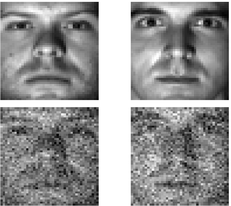
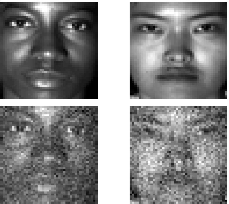
In this paper, we study two variants of the MC-UoS learning problem described by (2). In the first variant, all $m$ dimensions of each training sample in $\mathbf{Y}$ are observed and the geometry learning problem is exactly given by (2). In the second variant, it is assumed that some of the $m$ dimensions of each training sample in $\mathbf{Y}$ are unobserved (i.e., missing), which then requires a recharacterization of (2) for the learning problem to be well posed. We defer that recharacterization to Sec. III-C of the paper. In order to quantify the performance of our learning algorithms, we will resort to generation of noisy test data as follows. Given noiseless (synthetic or real) data sample $\mathbf{x}$ with $\|\mathbf{x}\|_{2}^{2}=1$, noisy test sample $\mathbf{z}$ is given by $\mathbf{z}=\mathbf{x}+\boldsymbol{\xi}$ with the additive noise $\boldsymbol{\xi}\sim\mathcal{N}(\boldsymbol{0},(\sigma_{te}^{2}/m)\mathbf{I}_{m})$. We will then report the metric of average approximation error of noisy test data using the learned subspaces for synthetic and real data. Finally, in the case of synthetic data drawn from an MC-UoS, we will also measure the performance of our algorithms in terms of average normalized subspace distances between the learned and the true subspaces. We defer a formal description of both these metrics to Sec. V-A1, which describes in detail the setup of our experiments.

Our second geometry learning problem corresponds to the case of high-dimensional data drawn from a mixture of nonlinear manifolds in the ambient space $\mathbb{R}^{m}$. The basic premise of our model in this case is that when data drawn from a mixture of nonlinear manifolds are mapped through a nonlinear map $\phi:\mathbb{R}^{m}\to\mathcal{F}$ to a higher-dimensional feature space $\mathcal{F}\subset\mathbb{R}^{\widetilde{m}}$ with $\widetilde{m}\ggg m$, then the $\phi$-mapped “images” of these data can be modeled as lying near an MC-UoS $\mathcal{M}_{L}$ in the feature space. In order to learn this model, we once again assume access to a collection of $N$ training samples, $\mathbf{Y}=[\mathbf{y}_{1},\dots,\mathbf{y}_{N}]\in\mathbb{R}^{m\times N}$, with the fundamental difference here being that the mapped training data $\phi(\mathbf{Y})=[\phi(\mathbf{y}_{1}),\dots,\phi(\mathbf{y}_{N})]$ are now assumed to be drawn from an MC-UoS $\mathcal{M}_{L}=\bigcup_{\ell=1}^{L}\mathcal{S}_{\ell}\subset\mathcal{G}_{\widetilde{m},s}\subset\mathcal{F}$. Here, we also make the simplified assumption that $\mathrm{rank}(\phi(\mathbf{Y}))=N$, which is justified as long as $\widetilde{m}\ggg N$ and no two training samples are identical. Our goal in this setting is to learn the (feature space) MC-UoS $\mathcal{M}_{L}$ using the training data $\mathbf{Y}$, which in theory can still be achieved by solving the following variant of (2):

where $l_{i}=\argmin_{\ell}\|\phi(\mathbf{y}_{i})-P_{\mathcal{S}_{\ell}}\phi(\mathbf{y}_{i})\|_{2}^{2}$ with $P_{\mathcal{S}_{\ell}}\phi(\mathbf{y}_{i})$ denoting the (orthogonal) projection of $\phi(\mathbf{y}_{i})$ onto the $s$-dimensional subspace $\mathcal{S}_{\ell}$ in $\mathbb{R}^{\widetilde{m}}$.

In practice, however, solving (3) directly is likely to be computationally intractable due to the extremely high dimensionality of the feature space. Instead, we are interested in solving the problem of MC-UoS learning in the feature space using the “kernel trick” [18], which involves transforming (3) into a learning problem that only requires evaluations of inner products in $\mathcal{F}$. Such a transformation can then be followed with the use of a Mercer kernel $\kappa$, which is a positive semidefinite function $\kappa:\mathbb{R}^{m}\times\mathbb{R}^{m}\to\mathbb{R}$ that satisfies $\kappa(\mathbf{y},\mathbf{y^{\prime}})=\langle\phi(\mathbf{y}),\phi(\mathbf{y^{\prime}})\rangle$ for all $\mathbf{y},\mathbf{y^{\prime}}\in\mathbb{R}^{m}$, to develop algorithms that can learn an MC-UoS in the feature space without explicit mapping of the training data to the feature space. We term the learning of an MC-UoS in the feature space using the kernel trick as metric-constrained kernel union-of-subspaces (MC-KUoS) learning. Similar to the case of MC-UoS learning, we consider two scenarios in this paper for MC-KUoS learning. The first one of these scenarios corresponds to the standard setup in which all $m$ dimensions of each training sample in $\mathbf{Y}$ are observed, while the second scenario corresponds to the case of “missing data” in which some dimensions of each training sample in $\mathbf{Y}$ remain unobserved. Finally, we will evaluate the proposed MC-KUoS learning algorithms using ($i$) the metric of average approximation error of noisy test data, and ($ii$) their clustering performance on training data having either complete or missing entries. We conclude here by pointing out that MC-KUoS learning invariably also leads us to the problem of finding the “pre-images” of data in the feature space induced by our chosen kernel (e.g., Gaussian or polynomial kernel) [9, 50], which will also be addressed in this paper.

In order to reduce the effects of noisy training data, we begin with a pre-processing step that centers the data matrix $\mathbf{Y}$.¹¹ 1 While such pre-processing is common in many geometry learning algorithms, it is not central to our framework. This involves defining the mean of the samples in $\mathbf{Y}$ as $\bar{\mathbf{y}}=\frac{1}{N}\sum_{i=1}^{N}\mathbf{y}_{i}$ and then subtracting this mean from $\mathbf{Y}$ to obtain the centered data $\widetilde{\mathbf{Y}}=[\widetilde{\mathbf{y}}_{1},\dots,\widetilde{\mathbf{y}}_{N}]$, where $\widetilde{\mathbf{y}}_{i}=\mathbf{y}_{i}-\bar{\mathbf{y}}$, $i=1,\dots,N$. Next, we focus on simplification of the optimization problem (2). To this end, we first define an $L\times N$ indicator matrix $\mathbf{W}$ that identifies memberships of the $\widetilde{\mathbf{y}}_{i}$’s in different subspaces, where $w_{\ell,i}=1$, $\ell=1,\dots,L$, $i=1,\dots,N$, if and only if $\widetilde{\mathbf{y}}_{i}$ is “closest” to subspace $\mathcal{S}_{\ell}$; otherwise, $w_{\ell,i}=0$. Mathematically,

Further, notice that $\|\mathbf{y}_{i}-P_{\mathcal{S}_{\ell}}\mathbf{y}_{i}\|_{2}^{2}$ in (2) can be rewritten as

where $\mathbf{D}_{\ell}\in\mathbb{R}^{m\times s}$ denotes an (arbitrary) orthonormal basis of $\mathcal{S}_{\ell}$. Therefore, defining $\mathbf{D}=[\mathbf{D}_{1},\dots,\mathbf{D}_{L}]$ to be a collection of orthonormal bases of $\mathcal{S}_{\ell}$’s, we can rewrite (2) as $(\mathbf{D},\mathbf{W})=\argmin_{\mathbf{D},\mathbf{W}}F_{1}(\mathbf{D},\mathbf{W})$ with the objective function $F_{1}(\mathbf{D},\mathbf{W})$ given by²² 2 Note that the minimization here is being carried out under the assumption of $\mathbf{D}_{\ell}$’s being orthonormal and $\mathbf{W}$ being described by (4).

Minimizing (6) simultaneously over $\mathbf{D}$ and $\mathbf{W}$ is challenging and is likely to be computationally infeasible. Instead, we adopt an alternate minimization approach [51, 52], which involves iteratively solving (6) by alternating between the following two steps: ($i$) minimizing $F_{1}(\mathbf{D},\mathbf{W})$ over $\mathbf{W}$ for a fixed $\mathbf{D}$, which we term as the subspace assignment step; and ($ii$) minimizing $F_{1}(\mathbf{D},\mathbf{W})$ over $\mathbf{D}$ for a fixed $\mathbf{W}$, which we term as the subspace update stage. To begin this alternate minimization, we start with an initial $\mathbf{D}$ in which each block $\mathbf{D}_{\ell}\in\mathbb{R}^{m\times s}$ is a random orthonormal basis. Next, we fix this $\mathbf{D}$ and carry out subspace assignment, which now amounts to solving for each $i=1,\dots,N$,

and then setting $w_{l_{i},i}=1$ and $w_{\ell,i}=0~\forall\ell\neq l_{i}$. In order to move to the subspace update step, we fix the matrix $\mathbf{W}$ and focus on optimizing $F_{1}(\mathbf{D},\mathbf{W})$ over $\mathbf{D}$. However, this step requires more attention since minimizing over the entire $\mathbf{D}$ at once will also lead to a large-scale optimization problem. We address this problem by once again resorting to block-coordinate descent (BCD) [51] and updating only one $\mathbf{D}_{\ell}$ at a time while keeping the other $\mathbf{D}_{p}$’s ($p\neq\ell$) fixed in (6). In this regard, suppose we are in the process of updating $\mathbf{D}_{\ell}$ for a fixed $\ell$ during the subspace update step. Define $\mathbf{c}_{\ell}=\{i\in\{1,\dots,N\}:w_{\ell,i}=1\}$ to be the set containing the indices of all $\widetilde{\mathbf{y}}_{i}$’s that are assigned to $\mathcal{S}_{\ell}$ (equivalently, $\mathbf{D}_{\ell}$) and let $\widetilde{\mathbf{Y}}_{\ell}=[\widetilde{\mathbf{y}}_{i}:i\in\mathbf{c}_{\ell}]$ be the corresponding $m\times|\mathbf{c}_{\ell}|$ matrix. Then it can be shown after some manipulations of (6) that updating $\mathbf{D}_{\ell}$ is equivalent to solving the following problem:

where $\mathcal{V}_{m,s}$ denotes the Stiefel manifold, defined as the collection of all $m\times s$ orthonormal matrices. Note that (8) has an intuitive interpretation. When $\lambda=0$, (8) reduces to the problem of finding a subspace that is closest to the remaining $L-1$ subspaces in our collection. When $\lambda=\infty$, (8) reduces to the PCA problem, in which case the learning problem (2) reduces to the subspace clustering problem studied in [41]. By selecting an appropriate $\lambda\in(0,\infty)$ in (8), we straddle the two extremes of subspace closeness and data approximation. In order to solve (8), we define an $m\times m$ symmetric matrix $\mathbf{A}_{\ell}=\sum_{p\neq\ell}{\mathbf{D}_{p}\mathbf{D}_{p}^{T}}+\frac{\lambda}{2}\widetilde{\mathbf{Y}}_{\ell}\widetilde{\mathbf{Y}}_{\ell}^{T}$. It then follows from [53] that (8) has a closed-form solution that involves eigen decomposition of $\mathbf{A}_{\ell}$. Specifically, $\mathbf{D}_{\ell}=\argmax\mathrm{tr}(\mathbf{D}_{\ell}^{T}\mathbf{A}_{\ell}\mathbf{D}_{\ell})$ is given by the first $s$ eigenvectors of $\mathbf{A}_{\ell}$ associated with its $s$-largest eigenvalues.

This completes our description of the subspace update step. We can now combine the subspace assignment and subspace update steps to fully describe our algorithm for MC-UoS learning. This algorithm, which we term metric-constrained union-of-subspaces learning (MiCUSaL), is given by Algorithm 1. In terms of the complexity of this algorithm in each iteration, notice that the subspace assignment step requires $\mathcal{O}(mLsN)$ operations. In addition, the total number of operations needed to compute the $\mathbf{A}_{\ell}$’s in each iteration is $\mathcal{O}(m^{2}(Ls+N))$. Finally, each iteration also requires $L$ eigen decompositions of $m\times m$ matrices, each one of which has $\mathcal{O}(m^{3})$ complexity. Therefore, the computational complexity of MiCUSaL in each iteration is given by $\mathcal{O}(m^{3}L+m^{2}N+m^{2}Ls+mLsN)$. We conclude this discussion by pointing out that we cannot guarantee convergence of MiCUSaL to a global optimal solution. However, since the objective function $F_{1}$ in (6) is bounded below by zero and MiCUSaL ensures that $F_{1}$ does not increase after each iteration, it follows that MiCUSaL iterates do indeed converge (possibly to one of the local optimal solutions). This local convergence, of course, will be a function of the initialization of MiCUSaL. In this paper, we advocate the use of random subspaces for initialization, while we study the impact of such random initialization in Sec. V-A.

The MiCUSaL algorithm described in Sec. III-A requires knowledge of the number of subspaces $L$ and the dimension of subspaces $s$. In practice, however, one cannot assume knowledge of these parameters a priori. Instead, one must estimate both the number and the dimension of subspaces from the training data themselves. In this section, we describe a generalization of the MiCUSaL algorithm that achieves this objective. Our algorithm, which we term adaptive MC-UoS learning (aMiCUSaL), requires only knowledge of loose upper bounds on $L$ and $s$, which we denote by $L_{max}$ and $s_{max}$, respectively.

The aMiCUSaL algorithm initializes with a collection of random orthonormal bases $\mathbf{D}=[\mathbf{D}_{1},\dots,\mathbf{D}_{L_{max}}]$, where each basis $\mathbf{D}_{\ell}$ is a point on the Stiefel manifold $\mathcal{V}_{m,s_{max}}$. Similar to the case of MiCUSaL, it then carries out the subspace assignment and subspace update steps in an iterative fashion. Unlike MiCUSaL, however, we also greedily remove redundant subspaces from our collection of subspaces $\{\mathcal{S}_{\ell}\}_{\ell=1}^{L_{max}}$ after each subspace assignment step. This involves removal of $\mathbf{D}_{\ell}$ from $\mathbf{D}$ if no signals in our training data get assigned to the subspace $\mathcal{S}_{\ell}$. This step of greedy subspace pruning ensures that only “active” subspaces survive before the subspace update step.

Once the aMiCUSaL algorithm finishes iterating between subspace assignment, subspace pruning, and subspace update, we move onto the step of greedy subspace merging, which involves merging of pairs of subspaces that are so close to each other that even a single subspace of the same dimension can be used to well approximate the data represented by the two subspaces individually.³³ 3 Note that the step of subspace merging is needed due to our lack of knowledge of the true number of subspaces in the underlying model. In particular, the assumption here is that the merging threshold $\epsilon_{min}$ in Algorithm 2 satisfies $\epsilon_{min}\ll\frac{\epsilon}{\sqrt{s}}$. In this step, we greedily merge pairs of closest subspaces as long as their normalized subspace distance is below a predefined threshold $\epsilon_{min}\in[0,1)$. Mathematically, the subspace merging step involves first finding the pair of subspaces $(\mathcal{S}_{\ell^{*}},\mathcal{S}_{p^{*}})$ that satisfies

We then merge $\mathcal{S}_{\ell^{*}}$ and $\mathcal{S}_{p^{*}}$ by setting $\mathbf{c}_{\ell^{*}}=\mathbf{c}_{\ell^{*}}\cup\mathbf{c}_{p^{*}}$ and $\widetilde{\mathbf{Y}}_{\ell^{*}}=[\widetilde{\mathbf{y}}_{i}:i\in\mathbf{c}_{\ell^{*}}]$, where $\mathbf{c}_{\ell^{*}},\mathbf{c}_{p^{*}}$ are as defined in Algorithm 1. By defining an $m\times m$ symmetric matrix $\mathbf{A}_{\ell^{*}}=\sum_{\ell\neq\ell^{*},p^{*}}{\mathbf{D}_{\ell}\mathbf{D}_{\ell}^{T}}+\frac{\lambda}{2}\widetilde{\mathbf{Y}}_{\ell^{*}}\widetilde{\mathbf{Y}}_{\ell^{*}}^{T}$, $\mathbf{D}_{\ell^{*}}$ is then set equal to the first $s_{max}$ eigenvectors of $\mathbf{A}_{\ell^{*}}$ associated with its $s_{max}$-largest eigenvalues. Finally, we remove $\mathbf{D}_{p^{*}}$ from $\mathbf{D}$. This process of finding the closest pair of subspaces and merging them is repeated until the normalized subspace distance between every pair of subspaces becomes greater than $\epsilon_{min}$. We assume without loss of generality that $\widehat{L}$ subspaces are left after this greedy subspace merging, where each $\mathcal{S}_{\ell}$ ($\ell=1,\dots,\widehat{L}$) is a subspace in $\mathbb{R}^{m}$ of dimension $s_{max}$.

After subspace merging, we move onto the step of estimation of the dimension, $s$, of the subspaces. To this end, we first estimate the dimension of each subspace $\mathcal{S}_{\ell}$, denoted by $s_{\ell}$, and then $s$ is selected as the maximum of these $s_{\ell}$’s. There have been many efforts in the literature to estimate the dimension of a subspace; see, e.g., [54, 55, 56, 57] for an incomplete list. In this paper, we focus on the method given in [54], which formulates the maximum likelihood estimator (MLE) of $s_{\ell}$. This is because: ($i$) the noise level is unknown in our problem, and ($ii$) the MLE in [54] has a simple form. However, the MLE of [54] is sensitive to noise. We therefore first apply a “smoothing” process before using that estimator. This involves first updating $\mathbf{W}$ (i.e., $\mathbf{c}_{\ell}$’s) using the updated $\mathbf{D}$ and “denoising” our data by projecting $\widetilde{\mathbf{Y}}_{\ell}$ onto $\mathcal{S}_{\ell}$, given by $\widehat{\mathbf{Y}}_{\ell}=\mathbf{D}_{\ell}\mathbf{D}_{\ell}^{T}\widetilde{\mathbf{Y}}_{\ell}$, and then using $\widehat{\mathbf{Y}}_{\ell}$ to estimate $s_{\ell}$. For a given column $\widehat{\mathbf{y}}$ in $\widehat{\mathbf{Y}}_{\ell}$ and a fixed number of nearest neighbors $k_{0}$, the unbiased MLE of $s_{\ell}$ with respect to $\widehat{\mathbf{y}}$ is given by [54]

where $\Gamma_{a}(\widehat{\mathbf{y}})$ is the $\ell_{2}$ distance between $\widehat{\mathbf{y}}$ and its $a$-th nearest neighbor in $\widehat{\mathbf{Y}}_{\ell}$. An estimate of $s_{\ell}$ can now be written as the average of all estimates with respect to every signal in $\widehat{\mathbf{Y}}_{\ell}$, i.e., $\widehat{s}_{\ell}^{k_{0}}=\frac{1}{|\mathbf{c}_{\ell}|}\sum_{i\in\mathbf{c}_{\ell}}\widehat{s}_{\ell}^{k_{0}}(\widehat{\mathbf{y}}_{i})$. In fact, as suggested in [54], we estimate $s_{\ell}$ by averaging over a range of $k_{0}=k_{1},\dots,k_{2}$, i.e.,

Once we get an estimate $s=\max_{\ell}\widehat{s}_{\ell}$, we trim each orthonormal basis by keeping only the first $s$ columns of each (ordered) orthonormal basis $\mathbf{D}_{\ell}$ in our collection, which is denoted by $\widehat{\mathbf{D}}_{\ell}$.⁴⁴ 4 Recall that the columns of $\mathbf{D}_{\ell}$ correspond to the eigenvectors of $\mathbf{A}_{\ell}$. Here, we are assuming that the order of these eigenvectors within $\mathbf{D}_{\ell}$ corresponds to the nonincreasing order of the eigenvalues of $\mathbf{A}_{\ell}$. Therefore, $\widehat{\mathbf{D}}_{\ell}$ comprises the eigenvectors of $\mathbf{A}_{\ell}$ associated with its $s$-largest eigenvalues. Given the bases $\{\widehat{\mathbf{D}}_{\ell}\in\mathbb{R}^{m\times s}\}_{\ell=1}^{\widehat{L}}$, we finally run MiCUSaL again that is initialized using these $\widehat{\mathbf{D}}_{\ell}$’s until it converges. Combining all the steps mentioned above, we can now formally describe adaptive MC-UoS learning (aMiCUSaL) in Algorithm 2.

In this section, we study MC-UoS learning for the case of training data having missing entries. To be specific, for each $\mathbf{y}_{i}$ in $\mathbf{Y}$, we assume to only observe its entries at locations given by the set $\mathbf{\Omega}_{i}\subset\{1,\dots,m\}$ with $|\mathbf{\Omega}_{i}|>s$, which is denoted by $[\mathbf{y}_{i}]_{\mathbf{\Omega}_{i}}\in\mathbb{R}^{|\mathbf{\Omega}_{i}|}$. Since we do not have access to the complete data, it is impossible to compute the quantities $\|\mathbf{y}_{i}-P_{\mathcal{S}_{\ell}}\mathbf{y}_{i}\|_{2}^{2}$ in (2) explicitly. But, it is shown in [58] that $\|[\mathbf{y}_{i}]_{\mathbf{\Omega}_{i}}-P_{\mathcal{S}_{\ell\mathbf{\Omega}_{i}}}[\mathbf{y}_{i}]_{\mathbf{\Omega}_{i}}\|_{2}^{2}$ for uniformly random $\mathbf{\Omega}_{i}$ is very close to $\frac{|\mathbf{\Omega}_{i}|}{m}\|\mathbf{y}_{i}-P_{\mathcal{S}_{\ell}}\mathbf{y}_{i}\|_{2}^{2}$ with very high probability as long as $|\mathbf{\Omega}_{i}|$ is slightly greater than $s$. Here, $P_{\mathcal{S}_{\ell\mathbf{\Omega}_{i}}}$ is defined as $P_{\mathcal{S}_{\ell\mathbf{\Omega}_{i}}}=[\mathbf{D}_{\ell}]_{\mathbf{\Omega}_{i},:}{([\mathbf{D}_{\ell}]_{\mathbf{\Omega}_{i},:})}^{\dagger}$ with ${([\mathbf{D}_{\ell}]_{\mathbf{\Omega}_{i},:})}^{\dagger}=\big([\mathbf{D}_{\ell}]_{\mathbf{\Omega}_{i},:}^{T}[\mathbf{D}_{\ell}]_{\mathbf{\Omega}_{i},:}\big)^{-1}[\mathbf{D}_{\ell}]_{\mathbf{\Omega}_{i},:}^{T}$. Motivated by this, we replace $\|\mathbf{y}_{i}-P_{\mathcal{S}_{\ell}}\mathbf{y}_{i}\|_{2}^{2}$ by $\frac{m}{|\mathbf{\Omega}_{i}|}\|[\mathbf{y}_{i}]_{\mathbf{\Omega}_{i}}-P_{\mathcal{S}_{\ell\mathbf{\Omega}_{i}}}[\mathbf{y}_{i}]_{\mathbf{\Omega}_{i}}\|_{2}^{2}$ in (2) and reformulate the MC-UoS learning problem as $(\mathbf{D},\mathbf{W})=\argmin_{\mathbf{D},\mathbf{W}}F_{2}(\mathbf{D},\mathbf{W})$ with the objective function $F_{2}(\mathbf{D},\mathbf{W})$ given by

As in Sec. III-A, we propose to solve this problem by making use of alternating minimization that comprises subspace assignment and subspace update steps. To this end, we again initialize $\mathbf{D}$ such that each block $\mathbf{D}_{\ell}\in\mathbb{R}^{m\times s}$ is a random orthonormal basis. Next, when $\mathbf{D}$ is fixed, subspace assignment corresponds to solving for each $i=1,\dots,N$,

and then setting $w_{l_{i},i}=1$ and $w_{\ell,i}=0~\forall\ell\neq l_{i}$. When $\mathbf{W}$ is fixed, we carry out subspace update using BCD again, in which case $\min_{\mathbf{D}}F_{2}(\mathbf{D},\mathbf{W})$ for a fixed $\mathbf{W}$ can be decoupled into $L$ distinct problems of the form $\mathbf{D}_{\ell}=\argmin_{\mathbf{D}_{\ell}\in\mathcal{V}_{m,s}}f_{2}(\mathbf{D}_{\ell})$, $\ell=1,\dots,L$, with

Here, $\mathbf{c}_{\ell}$ is as defined in Sec. III-A and $\mathbf{A}_{\ell}=\sum_{p\neq\ell}\mathbf{D}_{p}\mathbf{D}_{p}^{T}$. It is also easy to verify that $f_{2}(\mathbf{D}_{\ell})$ is invariant to the choice of the orthonormal basis of $\mathcal{S}_{\ell}$; hence, we can treat $\min_{\mathbf{D}_{\ell}\in\mathcal{V}_{m,s}}f_{2}(\mathbf{D}_{\ell})$ as an optimization problem on the Grassmann manifold [59]. Note that we can rewrite $f_{2}(\mathbf{D}_{\ell})$ as $f_{2}(\mathbf{D}_{\ell})=\sum_{q=0}^{|\mathbf{c}_{\ell}|}f_{2}^{(q)}(\mathbf{D}_{\ell})$, where $f_{2}^{(0)}(\mathbf{D}_{\ell})=-\mathrm{tr}(\mathbf{D}_{\ell}^{T}\mathbf{A}_{\ell}\mathbf{D}_{\ell})$ and $f_{2}^{(q)}(\mathbf{D}_{\ell})=\frac{\lambda m}{2|\mathbf{\Omega}_{{\mathbf{c}_{\ell}}_{(q)}}|}\|[\mathbf{y}_{{\mathbf{c}_{\ell}}_{(q)}}]_{\mathbf{\Omega}_{{\mathbf{c}_{\ell}}_{(q)}}}-P_{\mathcal{S}_{\ell\mathbf{\Omega}_{{\mathbf{c}_{\ell}}_{(q)}}}}[\mathbf{y}_{{\mathbf{c}_{\ell}}_{(q)}}]_{\mathbf{\Omega}_{{\mathbf{c}_{\ell}}_{(q)}}}\|_{2}^{2}$ for $q=1,\dots,|\mathbf{c}_{\ell}|$. In here, ${\mathbf{c}_{\ell}}_{(q)}$ denotes the $q$-th element in $\mathbf{c}_{\ell}$. In order to minimize $f_{2}(\mathbf{D}_{\ell})$, we employ incremental gradient descent procedure on Grassmann manifold [60], which performs the update with respect to a single component of $f_{2}(\mathbf{D}_{\ell})$ in each step. To be specific, we first compute the gradient of a single cost function $f_{2}^{(q)}(\mathbf{D}_{\ell})$ in $f_{2}(\mathbf{D}_{\ell})$, and move along a short geodesic curve in the gradient direction. For instance, the gradient of $f_{2}^{(0)}(\mathbf{D}_{\ell})$ is

Then the geodesic equation emanating from $\mathbf{D}_{\ell}$ in the direction $-\nabla f_{2}^{(0)}$ with a step length $\eta$ is given by [59]

where $\mathbf{U}_{\ell}\mathbf{\Sigma}_{\ell}\mathbf{V}_{\ell}^{T}$ is the SVD decomposition of $-\nabla f_{2}^{(0)}$. The update of $\mathbf{D}_{\ell}$ with respect to $f_{2}^{(q)}(\mathbf{D}_{\ell})$ $(q=1,\dots,|\mathbf{c}_{\ell}|)$ can be performed as in the GROUSE algorithm [61] but with a step size $\frac{\lambda m}{2|\mathbf{\Omega}_{{\mathbf{c}_{\ell}}_{(q)}}|}\eta$. In order for $f_{2}$ to converge, we also reduce the step size after each iteration [61]. We complete this discussion by presenting our learning algorithm for missing data in Algorithm 3, termed robust MC-UoS learning (rMiCUSaL). By defining $T=\max_{i}|\mathbf{\Omega}_{i}|$, the subspace assignment step of rMiCUSaL requires $\mathcal{O}(TLs^{2}N)$ flops in each iteration [61]. Computing the $\mathbf{A}_{\ell}$’s in each iteration requires $\mathcal{O}(m^{2}Ls)$ operations. Next, the cost of updating each $\mathbf{D}_{\ell}$ with respect to $f_{2}^{(0)}(\mathbf{D}_{\ell})$ is $\mathcal{O}(m^{3})$, while it is $\mathcal{O}(ms+Ts^{2})$ with respect to $f_{2}^{(q)}(\mathbf{D}_{\ell})$ for $q\neq 0$ [61]. It therefore follows that the computational complexity of rMiCUSaL in each iteration is $\mathcal{O}(m^{3}L+m^{2}Ls+msN+TLs^{2}N)$. We refer the reader to Sec. V-A for exact running time of rMiCUSaL on training data.

References

- [1] T. Wu and W. U. Bajwa, “Revisiting robustness of the union-of-subspaces model for data-adaptive learning of nonlinear signal models,” in Proc. IEEE Int. Conf. Acoustics, Speech and Signal Processing (ICASSP), 2014, pp. 3390–3394.
- [2] ——, “Subspace detection in a kernel space: The missing data case,” in Proc. IEEE Statistical Signal Processing Workshop (SSP), 2014, pp. 93–96.
- [3] ——, “Metric-constrained kernel union of subspaces,” in Proc. IEEE Int. Conf. Acoustics, Speech and Signal Processing (ICASSP), 2015.
- [4] H. Hotelling, “Analysis of a complex of statistical variables into principal components,” J. Educ. Psych., vol. 24, pp. 417–441, 498–520, 1933.
- [5] T. F. Cox and M. A. A. Cox, Multidimensional scaling. Chapman & Hall, 2000.
- [6] S. T. Roweis and L. K. Saul, “Nonlinear dimensionality reduction by locally linear embedding,” Science, vol. 290, pp. 2323–2326, 2000.
- [7] M. Elad, R. Goldenberg, and R. Kimmel, “Low bit-rate compression of facial images,” IEEE Trans. Image Process., vol. 16, no. 9, pp. 2379–2383, 2007.
- [8] R. G. Baraniuk, V. Cevher, and M. B. Wakin, “Low-dimensional models for dimensionality reduction and signal recovery: A geometric perspective,” Proc. IEEE, vol. 98, no. 6, pp. 959–971, 2010.
- [9] S. Mika, B. Schölkopf, A. J. Smola, K.-R. Müller, M. Scholz, and G. Rätsch, “Kernel PCA and de-noising in feature spaces,” in Advances in Neural Information Processing Systems (NIPS), 1998, pp. 536–542.
- [10] M. Elad and M. Aharon, “Image denoising via sparse and redundant representations over learned dictionaries,” IEEE Trans. Image Process., vol. 15, no. 12, pp. 3736–3745, 2006.
- [11] M. A. Turk and A. P. Pentland, “Face recognition using eigenfaces,” in Proc. IEEE Conf. Computer Vision and Pattern Recognition (CVPR), 1991, pp. 586–591.
- [12] D. L. Swets and J. Weng, “Using discriminant eigenfeatures for image retrieval,” IEEE Trans. Pattern Anal. Mach. Intell., vol. 18, no. 8, pp. 831–836, 1996.
- [13] J. Wright, A. Y. Yang, A. Ganesh, S. S. Sastry, and Y. Ma, “Robust face recognition via sparse representation,” IEEE Trans. Pattern Anal. Mach. Intell., vol. 31, no. 2, pp. 210–227, 2009.
- [14] J. Mairal, F. Bach, and J. Ponce, “Task-driven dictionary learning,” IEEE Trans. Pattern Anal. Mach. Intell., vol. 34, no. 4, pp. 791–804, 2012.
- [15] S. Rao, R. Tron, R. Vidal, and Y. Ma, “Motion segmentation in the presence of outlying, incomplete, or corrupted trajectories,” IEEE Trans. Pattern Anal. Mach. Intell., vol. 32, no. 10, pp. 1832–1845, 2010.
- [16] E. Elhamifar and R. Vidal, “Sparse subspace clustering: Algorithm, theory, and applications,” IEEE Trans. Pattern Anal. Mach. Intell., vol. 35, no. 11, pp. 2765–2781, 2013.
- [17] H. H. Harman, Modern factor analysis. University of Chicago Press, 1976.
- [18] B. Schölkopf, A. J. Smola, and K.-R. Müller, “Nonlinear component analysis as a kernel eigenvalue problem,” Neural Comput., vol. 10, no. 5, pp. 1299–1319, 1998.
- [19] M. Aharon, M. Elad, and A. Bruckstein, “K-SVD: An algorithm for designing overcomplete dictionaries for sparse representation,” IEEE Trans. Signal Process., vol. 54, no. 11, pp. 4311–4322, 2006.
- [20] Y. C. Eldar and M. Mishali, “Robust recovery of signals from a structured union of subspaces,” IEEE Trans. Inf. Theory, vol. 55, no. 11, pp. 5302–5316, 2009.
- [21] M. W. Marcellin, M. J. Gormish, A. Bilgin, and M. P. Boliek, “An overview of JPEG-2000,” in Proc. IEEE Data Compression Conf. (DCC), 2000, pp. 523–541.
- [22] J.-L. Starck, E. J. Candès, and D. L. Donoho, “The curvelet transform for image denoising,” IEEE Trans. Image Process., vol. 11, no. 6, pp. 670–684, 2002.
- [23] T. Zhang, A. Szlam, and G. Lerman, “Median K-flats for hybrid linear modeling with many outliers,” in Proc. IEEE Int. Conf. Computer Vision Workshops, 2009, pp. 234–241.
- [24] B. V. Gowreesunker and A. H. Tewfik, “Learning sparse representation using iterative subspace identification,” IEEE Trans. Signal Process., vol. 58, no. 6, pp. 3055–3065, 2010.
- [25] L. Balzano, A. Szlam, B. Recht, and R. Nowak, “K-subspaces with missing data,” in Proc. IEEE Statistical Signal Processing Workshop (SSP), 2012, pp. 612–615.
- [26] W. Hong, J. Wright, K. Huang, and Y. Ma, “Multiscale hybrid linear models for lossy image representation,” IEEE Trans. Image Process., vol. 15, no. 12, pp. 3655–3671, 2006.
- [27] K. Pearson, “On lines and planes of closest fit to systems of points in space,” Philos. Mag., vol. 2, no. 6, pp. 559–572, 1901.
- [28] K. Fukunaga, Introduction to statistical pattern recognition. Academic Press, 1990.
- [29] B. Schölkopf, A. J. Smola, and K.-R. Müller, “Kernel principal component analysis,” Advances in kernel methods: support vector learning, pp. 327–352, 1999.
- [30] M. Belkin and P. Niyogi, “Laplacian eigenmaps for dimensionality reduction and data representation,” Neural Comput., vol. 15, no. 6, pp. 1373–1396, 2003.
- [31] J. Ham, D. D. Lee, S. Mika, and B. Schölkopf, “A kernel view of the dimensionality reduction of manifolds,” in Proc. Int. Conf. Machine Learning (ICML), 2004, pp. 47–54.
- [32] R. Vidal, Y. Ma, and S. Sastry, “Generalized principal component analysis (GPCA),” IEEE Trans. Pattern Anal. Mach. Intell., vol. 27, no. 12, pp. 1945–1959, 2005.
- [33] L. Zelnik-Manor, K. Rosenblum, and Y. C. Eldar, “Dictionary optimization for block-sparse representations,” IEEE Trans. Signal Process., vol. 60, no. 5, pp. 2386–2395, 2012.
- [34] M. Soltanolkotabi and E. J. Candès, “A geometric analysis of subspace clustering with outliers,” Ann. Stat., vol. 40, no. 4, pp. 2195–2238, 2012.
- [35] E. L. Dyer, A. C. Sankaranarayanan, and R. G. Baraniuk, “Greedy feature selection for subspace clustering,” J. Mach. Learn. Res., vol. 14, pp. 2487–2517, 2013.
- [36] R. Heckel and H. Bölcskei, “Robust subspace clustering via thresholding,” arXiv:1307.4891, 2013.
- [37] M. Soltanolkotabi, E. Elhamifar, and E. J. Candès, “Robust subspace clustering,” Ann. Stat., vol. 42, no. 2, pp. 669–699, 2014.
- [38] T. Zhang, A. Szlam, Y. Wang, and G. Lerman, “Hybrid linear modeling via local best-fit flats,” Int. J. Comput. Vis., vol. 100, no. 3, pp. 217–240, 2012.
- [39] Z. Ghahramani and G. E. Hinton, “The EM algorithm for mixtures of factor analyzers,” CRG-TR-96-1, University of Toronto, Tech. Rep., 1997.
- [40] J. Wright, Y. Ma, J. Mairal, G. Sapiro, T. S. Huang, and S. Yan, “Sparse representation for computer vision and pattern recognition,” Proc. IEEE, vol. 98, no. 6, pp. 1031–1044, 2010.
- [41] J. Ho, M.-H. Yang, J. Lim, K.-C. Lee, and D. Kriegman, “Clustering appearances of objects under varying illumination conditions,” in Proc. IEEE Conf. Computer Vision and Pattern Recognition (CVPR), 2003, pp. 11–18.
- [42] Y. M. Lu and M. N. Do, “A theory for sampling signals from a union of subspaces,” IEEE Trans. Signal Process., vol. 56, no. 6, pp. 2334–2345, 2008.
- [43] L. Wang, X. Wang, and J. Feng, “Subspace distance analysis with application to adaptive Bayesian algorithm for face recognition,” Pattern Recognition, vol. 39, no. 3, pp. 456–464, 2006.
- [44] X. Sun, L. Wang, and J. Feng, “Further results on the subspace distance,” Pattern Recognition, vol. 40, no. 1, pp. 328–329, 2007.
- [45] L. Wolf and A. Shashua, “Kernel principal angles for classification machines with applications to image sequence interpretation,” in Proc. IEEE Conf. Computer Vision and Pattern Recognition (CVPR), 2003, pp. 635–640.
- [46] R. Kohavi, “A study of cross-validation and bootstrap for accuracy estimation and model selection,” in Proc. Int. Joint Conf. Artificial Intelligence (IJCAI), 1995, pp. 1137–1143.
- [47] K. Pelckmans, J. De Brabanter, J. A. K. Suykens, and B. De Moor, “Convex clustering shrinkage,” in Statistics and Optimization of Clustering Workshop (PASCAL), 2005.
- [48] K.-C. Lee, J. Ho, and D. Kriegman, “Acquiring linear subspaces for face recognition under variable lighting,” IEEE Trans. Pattern Anal. Mach. Intell., vol. 27, no. 5, pp. 684–698, 2005.
- [49] R. Basri and D. W. Jacobs, “Lambertian reflectance and linear subspaces,” IEEE Trans. Pattern Anal. Mach. Intell., vol. 25, no. 2, pp. 218–233, 2003.
- [50] J. T.-Y. Kwok and I. W.-H. Tsang, “The pre-image problem in kernel methods,” IEEE Trans. Neural Netw., vol. 15, no. 6, pp. 1517–1525, 2004.
- [51] D. P. Bertsekas, Nonlinear programming. Athena Scientific, 1999.
- [52] J. C. Bezdek and R. J. Hathaway, “Convergence of alternating optimization,” Neural Parallel Sci. Comput., vol. 11, no. 4, pp. 351–368, 2003.
- [53] E. Kokiopoulou, J. Chen, and Y. Saad, “Trace optimization and eigenproblems in dimension reduction methods,” Numer. Linear Algebra Appl., vol. 18, no. 3, pp. 565–602, 2011.
- [54] E. Levina and P. J. Bickel, “Maximum likelihood estimation of intrinsic dimension,” in Advances in Neural Information Processing Systems (NIPS), 2004, pp. 777–784.
- [55] J. M. Bioucas-Dias and J. M. P. Nascimento, “Hyperspectral subspace identification,” IEEE Trans. Geosci. Remote Sens., vol. 46, no. 8, pp. 2435–2445, 2008.
- [56] S. Kritchman and B. Nadler, “Determining the number of components in a factor model from limited noisy data,” Chemometr. Intell. Lab. Syst., vol. 94, no. 1, pp. 19–32, 2008.
- [57] P. O. Perry and P. J. Wolfe, “Minimax rank estimation for subspace tracking,” IEEE J. Sel. Topics Signal Process., vol. 4, no. 3, pp. 504–513, 2010.
- [58] L. Balzano, B. Recht, and R. Nowak, “High-dimensional matched subspace detection when data are missing,” in Proc. IEEE Int. Symp. Inf. Theory (ISIT), 2010, pp. 1638–1642.
- [59] A. Edelman, T. A. Arias, and S. T. Smith, “The geometry of algorithms with orthogonality constraints,” SIAM J. Matrix Anal. Appl., vol. 20, no. 2, pp. 303–353, 1998.
- [60] A. Nedić and D. P. Bertsekas, “Incremental subgradient methods for nondifferentiable optimization,” SIAM J. Optim., vol. 12, no. 1, pp. 109–138, 2001.
- [61] L. Balzano, R. Nowak, and B. Recht, “Online identification and tracking of subspaces from highly incomplete information,” in Proc. Allerton Conf. Communication, Control, and Computing, 2010, pp. 704–711.
- [62] B. Eriksson, L. Balzano, and R. Nowak, “High-rank matrix completion,” in Proc. Int. Conf. Artificial Intelligence and Statistics (AISTATS), 2012, pp. 373–381.
- [63] C. J. C. Burges, “Simplified support vector decision rules,” in Proc. Int. Conf. Machine Learning (ICML), 1996, pp. 71–77.
- [64] Y. Rathi, S. Dambreville, and A. Tannenbaum, “Statistical shape analysis using kernel PCA,” in Proc. SPIE, vol. 6064, 2006.
- [65] J. J. Hull, “A database for handwritten text recognition research,” IEEE Trans. Pattern Anal. Mach. Intell., vol. 16, no. 5, pp. 550–554, 1994.
- [66] S. P. Lloyd, “Least squares quantization in PCM,” IEEE Trans. Inf. Theory, vol. 28, no. 2, pp. 129–137, 1982.
- [67] U. von Luxburg, “A tutorial on spectral clustering,” Stat. Comput., vol. 17, no. 4, pp. 395–416, 2007.
- [68] F. R. Bach, G. R. G. Lanckriet, and M. I. Jordan, “Multiple kernel learning, conic duality, and the SMO algorithm,” in Proc. Int. Conf. Machine Learning (ICML), 2004, pp. 41–48.
- [69] G. R. G. Lanckriet, N. Cristianini, P. Bartlett, L. E. Ghaoui, and M. I. Jordan, “Learning the kernel matrix with semidefinite programming,” J. Mach. Learn. Res., vol. 5, pp. 27–72, 2004.
- [70] C. Cortes, M. Mohri, and A. Rostamizadeh, “Learning non-linear combinations of kernels,” in Advances in Neural Information Processing Systems (NIPS), 2009, pp. 396–404.
- [71] M. Kloft, U. Brefeld, S. Sonnenburg, and A. Zien, “-norm multiple kernel learning,” J. Mach. Learn. Res., vol. 12, pp. 953–997, 2011.
- [72] C. McDiarmid, “On the method of bounded differences,” Surveys in Combinatorics, vol. 141, pp. 148–188, 1989.
![[Uncaptioned image]](1412.6808v2/Wu_Photo.png) |
Tong Wu received BE degree in Instrument Science and Engineering from Shanghai Jiao Tong University, China in 2009, and MS degree in Electrical Engineering from Duke University in 2011. Since September 2012, he has been working towards the PhD degree at the Department of Electrical and Computer Engineering, Rutgers, The State University of New Jersey. His research interests include high-dimensional data analysis, statistical signal processing, image and video processing, and machine learning. |
![[Uncaptioned image]](1412.6808v2/Bajwa_Photo.png) |
Waheed U. Bajwa received BE (with Honors) degree in electrical engineering from the National University of Sciences and Technology, Pakistan in 2001, and MS and PhD degrees in electrical engineering from the University of Wisconsin-Madison in 2005 and 2009, respectively. He was a Postdoctoral Research Associate in the Program in Applied and Computational Mathematics at Princeton University from 2009 to 2010, and a Research Scientist in the Department of Electrical and Computer Engineering at Duke University from 2010 to 2011. He is currently an Assistant Professor in the Department of Electrical and Computer Engineering at Rutgers University. His research interests include harmonic analysis, high-dimensional statistics, machine learning, statistical signal processing, and wireless communications. Dr. Bajwa has more than three years of industry experience, including a summer position at GE Global Research, Niskayuna, NY. He received the Best in Academics Gold Medal and President’s Gold Medal in Electrical Engineering from the National University of Sciences and Technology in 2001, the Morgridge Distinguished Graduate Fellowship from the University of Wisconsin-Madison in 2003, the Army Research Office Young Investigator Award in 2014, and the National Science Foundation CAREER Award in 2015. He co-guest edited a special issue of Elsevier Physical Communication Journal on “Compressive Sensing in Communications” (2012), and co-chaired CPSWeek 2013 Workshop on Signal Processing Advances in Sensor Networks and IEEE GlobalSIP 2013 Symposium on New Sensing and Statistical Inference Methods. He currently serves as the Publicity and Publications Chair of IEEE CAMSAP 2015, and is an Associate Editor of the IEEE Signal Processing Letters. |