Principal Sensitivity Analysis

Before introducing the PSA, we describe the original sensitivity map introduced in [10]. Let $d$ be the dimension of the input space, and let $f:\mathbb{R}^{d}\to\mathbb{R}$ be the classifier function obtained from supervised training. In the case of SVM, $f$ may be the discriminant function. In the case of nonlinear neural networks, $f$ may represent the function (or log of the function) that maps the input to the output of a unit in the final layer. We are interested in the expected sensitivity of $f$ with respect to the $i$-th input feature. This can be written as

where $q$ is the distribution over the input space. In actual implementation, the integral (1) is computed with the empirical distribution $q$ of the test dataset. Now, the vector

of these values will give us an intuitive measure for the degree of importance that the classifier attaches to each input. Kjems et al. [10] defined $\vec{s}$ as sensitivity map over the set of input features.

Here, we generalize the definition (1). We define $s(\vec{v})$ as the sensitivity of $f$ in arbitrary direction $\vec{v}:=\sum_{i}^{d}v_{i}\vec{e}_{i}$, where $\vec{e}_{i}$ denotes the $i$-th standard basis in $\mathbb{R}^{d}$:

Recall that the directional derivative is defined by

Note that when we define the sensitivity inner product

we can rewrite $s(\vec{v})$ with the corresponding sensitivity norm, as follows:

This inner product defines the kernel metric corresponding to the positive definite matrix $\vec{K}$ with $ij$-th entry given by $K_{ij}:=\left\langle\vec{e}_{i},\vec{e}_{j}\right\rangle_{s}$. This allows us to write

The classical setting (2) was developed in order to quantify the sensitivity of $f$ with respect to each individual input feature. We attempt to generalize this idea and seek the combination of the input features for which $f$ is most sensitive, or the combination of the input features that is “principal” in the evaluation of the sensitivity of $f$. We can quantify such combination by the vector $\vec{v}$, solving the following optimization problem about $\vec{v}$:

The solution to this problem is simply the maximal eigenvector $\pm\vec{v}^{*}$ of $\vec{K}$. Note that $v_{i}$ represents the contribution of the $i$-th input feature to this principal combination, and this gives rise to the map over the set of all input features. As such, we can say that $\vec{v}$ is the principal sensitivity map (PSM) over the set of input features. From now on, we call $\vec{s}$ in the classical definition (2) as the standard sensitivity map and make the distinction. The magnitude of $v_{i}$ represents the extent to which $f$ is sensitive to the $i$-th input feature, and the sign of $v_{i}$ will tell us the relative direction to which the input feature influences $f$. The new map is thus richer in information than the standard sensitivity map. In Section 3.1 we will demonstrate the benefit of this extra information.

In order to demonstrate the effectiveness of the PSA, we applied the analysis to the classifiers that we trained with artificial data and MNIST data. Our artificial data is a simplified version of the MNIST data in which the object’s orientation and positioning are registered from the beginning. All samples in the artificial data are constructed by adding noises to the common set of templates representing the numerics from $0$ through $9$ (Fig. 1). We then fabricated the artificial noise in three steps: we (1) flipped the bit of each pixel in the template picture with probability $p=0.2$, (2) added Gaussian noise $\mathcal{N}(0,0.1)$ to the intensity, and (3) truncated the negative intensities. The sample size was set to be equal to that of MNIST. Our training data, validation data, and test data consisted respectively of 50,000, 10,000, and 10,000 sample patterns.

Using the artificial dataset above and the standard MNIST, we trained a feed forward neural network for the classification of ten numerics. In Table 1, we provide the structure of the neural network and its performance over each dataset. For either dataset, the training was conducted via stochastic gradient descent with constant learning rate. We also adopted a dropout method [13] only for the training on the MNIST dataset. The output from each unit in the final layer is given by the posterior probability of each class $c$. For computational purpose, we transform this output by $\log$:

where $Y$ is, in the model governing the neural network, a random variable representing the class that the classifier assigns to the input $\vec{x}$. We then constructed the PSM and the standard sensitivity map for the $f_{c}$ given above.

We will describe three ways in which the PSA can be superior to the analysis based on standard sensitivity map.

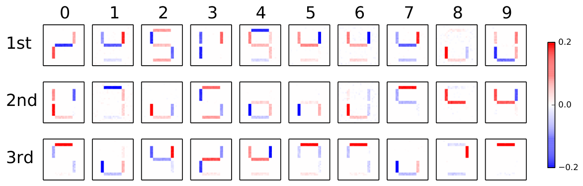
Fig. 2 compares the PSM and standard sensitivity map, which were both obtained from the common neural networks trained for the same 10-class classification problem. The color intensity of $i$-th pixel represents the magnitude of $v_{i}$. Both maps capture the characters that the “colorless” rims and likewise “colorless” regions enclosed by edges are insignificant in the classification. Note that the (1st) PSM distinguishes the types of sensitivities by their sign. For each numeral, the PSM assigns opposite signs to “the edges whose presence is crucial in the characterization of the very numeral” and “the edges whose absence is crucial in the numeral’s characterization.” This information is not featured in the standard sensitivity map. For instance, in the sensitivity map for the numeral $1$, the two edges on the right and the rest of the edges have the opposite sensitivity. As a result, we can verify the red figure of $1$ in its PSM. We are able to clearly identify the unbroken figures of $2,4,5$ and $9$ in their corresponding PSM as well. We see that, with the extra information regarding the sign of the sensitivity over each pixel, PSM can provide us with much richer information than the standard counterpart.

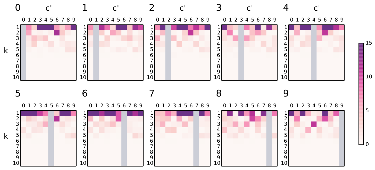
Next, we will show the benefits of sub-principal sensitivity maps computed from PSA. Fig. 3(a) shows the 1st PSM through the 3rd PSM for the numerals $0$ and $9$.¹¹ 1 We list the PSMs for all the numerals ($0,\dots,9$) in the Appendix. In order to show how this extra information benefits us in visualization of the classification problem, we consider the following “local” sensitivity map integrated over the samples from a particular pair of classes:

where $q_{c,c^{\prime}}$ is the empirical distribution over the set of samples generated from the classes $c$ and $c^{\prime}$. To get the intuition about this map, note that this value for $(c,c^{\prime})=(9,4)$ can also be pictorially written as

$\displaystyle\lim_{\varepsilon\rightarrow 0}E_{\{9,4\}}\left[\left(\frac{\log P\left(Y=\parbox{19.4703pt}{\hbox{ \includegraphics[width=12.80365pt]{fig/class_9.pdf} }}|\parbox{19.4703pt}{\hbox{ \includegraphics[width=12.80365pt]{fig/sample_4.pdf} }}+\varepsilon\vec{v}\right)-\log P\left(Y=\parbox{19.4703pt}{\hbox{ \includegraphics[width=12.80365pt]{fig/class_9.pdf} }}|\parbox{19.4703pt}{\hbox{ \includegraphics[width=12.80365pt]{fig/sample_4.pdf} }}\right)}{\varepsilon}\right)^{2}\right],$

(13)

where $\vec{v}$ can be the 3rd PSM of class 9, , for example. If $\vec{v}_{k}$ is the $k$-th PSM of the classifier, then $s_{c,c^{\prime}}(\vec{v}_{k})$ quantifies the sensitivity of the machine’s answer to the binary classification problem of “$c$ vs $c^{\prime}$” with respect to the perturbation of the input in the direction of $\vec{v}_{k}$. By looking at this value for each $k$, we may visualize the ways that the classifier deals with the binary classification problem. Such visualization may aid us in learning from the classifiers the way to distinguish one class from another. Fig. 3(b) shows the values of $s_{c,c^{\prime}}(\vec{v}_{k})$ for $c\in\{0,9\}$ and $k\in\{1,\dots,10\}$. We could see in the figure that, for the case of $(c,c^{\prime})=(9,4)$, $s_{c,c^{\prime}}(\vec{v}_{3})$ was larger than $s_{c,c^{\prime}}(\vec{v}_{1})$. This suggests that the 3rd PSM is more helpful than the 1st PSM for distinguishing $4$ from $9$. We can actually verify this fact by observing that the 3rd PSM is especially intense at the top most edge, which can alone differentiate $4$ from $9$. We are able to confirm many other cases in which the sub-principal sensitivity maps were more helpful in capturing the characters in binary classification problems than the 1st PSM. Thus, PSA can provide us with the knowledge of the classifiers that was inaccessible with the previous method based on the standard sensitivity map.

Finally, we demonstrate the usefulness of formulation (8) in the construction of sparse and intuitive sensitivity map. Fig. 4 depicts the sensitivity maps obtained from the application of our sparse PSA in (10) to the data above. Note that the sparse PSA not only washes away rather irrelevant pixels from the canvas, but it also assigns very high intensity to essential pixels. With these “localized” maps, we can better understand the discriminative features utilized by the trained classifiers.

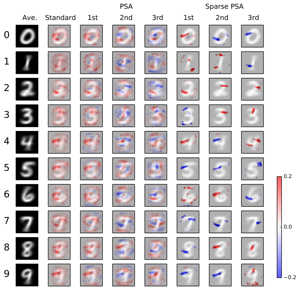
We trained a nonlinear neural network-based classifier on the MNIST dataset, which consists of hand-written digits from $0$ through $9$. We then analyzed the trained classifier with our PSA. This dataset illuminates a particular challenge to be confronted in the application of the PSA. By default, hand-written objects do not share common displacement and orientation. Without an appropriate registration of input space, the meaning of each pixel can vary across the samples, making the visualization unintuitive. This is typical in some of the real-world classification problems. In the fields of applied science, standard registration procedure is often applied to the dataset before the construction of the classifiers. For example, in neuroimaing, one partitions the image data into anatomical regions after registration based on the standard brain, and represents each one of them by a group of voxels. In other areas of science, one does not necessarily have to face such problems. In genetics, data can be naturally partitioned into genes [14]. Likewise, in meteorology, 3D dataset is often translated into voxel structures, and a group of voxels may represent geographical region of specific terrain [15]. In this light, the digit recognition in unregistered MNIST data may not be an appropriate example for showing the effectiveness of our visualization method. For the reason that we will explain later, registration of multiclass dataset like MNIST can be difficult. We chose MNIST dataset here because it is familiar in the community of machine learning. Fig. 5 summarizes the results. Both the standard sensitivity map and the PSM were able to capture the character that outer rims are rather useless in the classification.

Fig. 6 shows the values of $s_{c,c^{\prime}}(\vec{v}_{k})$. We can verify that small numbers of PSMs are complementing each other in their contributions to the binary classifications.

We also applied sparse PSA to the classifier with $p=3$ and $\lambda=40$ (Fig. 5). We see that the sparse PSA highlights the essential pixels much more clearly than the normal PSA.

Since the orientation and position of each numeral pattern varies across the samples in this dataset, input dimensions hold different meanings in different samples. To perform more effective visualization, we would need registration to adjust each numeral pattern to a common standard template. This problem might not be straightforward, since one must prepare different templates for different numeral patterns. An elegant standardization suitable for our PSA-based visualization remains as a future study.

References

- [1] Taigman, Y., Yang, M., Ranzato, M., Wolf, L.: Deepface: Closing the gap to human-level performance in face verification. In: Proceedings of the IEEE Conference on Computer Vision and Pattern Recognition (CVPR). (2014) 1701–1708
- [2] Horikawa, T., Tamaki, M., Miyawaki, Y., Kamitani, Y.: Neural decoding of visual imagery during sleep. Science 340 (2013) 639–642
- [3] Uberbacher, E.C., Mural, R.J.: Locating protein-coding regions in human DNA sequences by a multiple sensor-neural network approach. Proceedings of the National Academy of Sciences 88 (1991) 11261–11265
- [4] Hinton, G.E.: Dark knowledge. Presented as the keynote in BayLearn (2014)
- [5] Baehrens, D., Schroeter, T., Harmeling, S., Kawanabe, M., Hansen, K., Muller, K.R.: How to explain individual classification decisions. The Journal of Machine Learning Research 11 (2010) 1803–1831
- [6] Rasmussen, P.M., Madsen, K.H., Lund, T.E., Hansen, L.K.: Visualization of nonlinear kernel models in neuroimaging by sensitivity maps. NeuroImage 55 (2011) 1120–1131
- [7] LaConte, S., Strother, S., Cherkassky, V., Anderson, J., Hu, X.: Support vector machines for temporal classification of block design fMRI data. NeuroImage 26 (2005) 317–329
- [8] Zurada, J.M., Malinowski, A., Cloete, I.: Sensitivity analysis for minimization of input data dimension for feedforward neural network. In: Proceedings of the IEEE International Symposium on Circuits and Systems (ISCAS). Volume 6. (1994) 447–450
- [9] Zurada, J.M., Malinowski, A., Usui, S.: Perturbation method for deleting redundant inputs of perceptron networks. Neurocomputing 14 (1997) 177–193
- [10] Kjems, U., Hansen, L.K., Anderson, J., Frutiger, S., Muley, S., Sidtis, J., Rottenberg, D., Strother, S.C.: The quantitative evaluation of functional neuroimaging experiments: mutual information learning curves. NeuroImage 15 (2002) 772–786
- [11] Jenatton, R., Obozinski, G., Bach, F.: Structured sparse principal component analysis. In: Proceedings of the International Conference on Artificial Intelligence and Statistics (AISTATS). Volume 9. (2010) 366–373
- [12] Pedregosa, F., Varoquaux, G., Gramfort, A., Michel, V., Thirion, B., Grisel, O., Blondel, M., Prettenhofer, P., Weiss, R., Dubourg, V., Vanderplas, J., Passos, A., Cournapeau, D., Brucher, M., Perrot, M., Duchesnay, E.: Scikit-learn: Machine Learning in Python. The Journal of Machine Learning Research 12 (2012) 2825–2830
- [13] Hinton, G.E., Srivastava, N., Krizhevsky, A., Sutskever, I., Salakhutdinov, R.R.: Improving neural networks by preventing co-adaptation of feature detectors. arXiv preprint arXiv:1207.0580 (2012) 1–18
- [14] Yukinawa, N., Oba, S., Kato, K., Ishii, S.: Optimal aggregation of binary classifiers for multiclass cancer diagnosis using gene expression profiles. IEEE/ACM Transactions on Computational Biology and Bioinformatics 6 (2009) 333–343
- [15] Kontos, D., Megalooikonomou, V.: Fast and effective characterization for classification and similarity searches of 2D and 3D spatial region data. Pattern Recognition 38 (2005) 1831–1846
Appendix
In this section we list the figures that we omitted in the main text.