Timelike pion form factor in lattice QCD
Abstract
We perform a nonperturbative lattice calculation of the complex phase and modulus of the pion form factor in the timelike momentum region using the finite-volume technique. We use two ensembles of -flavor overlap fermion at pion masses = 380 and 290 MeV. By calculating the correlators in the center-of-mass and three moving frames, we obtain the form factor at ten different values of the timelike momentum transfer around the vector resonance. We compare the results with the phenomenological model of Gounaris-Sakurai and its variant.
Keywords:
timelike pion form factor, finite-volume method, lattice QCDpacs
12.38.Gc 13.75.Lb 13.40.GpI Introduction
Lattice quantum chromodynamics (QCD) has been successful at providing first-principles calculations of various physical quantities, among which the calculations of the so-called gold-plated quantities, such as the lowest-lying hadron masses, decay constants and matrix elements with one hadron or vacuum as the initial or final state, are carried out with controlled errors. On the other hand, there are many interesting physical observables that are beyond gold-plated. An interesting example is that of transition amplitudes involving non-QCD initial/final states, such as the amplitudes for [1] and [2, 3, 4, 5, 6]. Another example is the decay [7, 8, 9], where the final state consists of multiple strongly interacting pions. For such cases, the finite-volume correction to the two-body state must be properly taken into account [10].
For the decay, the main efforts have been made to reproduce the physical amplitude where the center-of-mass (CM) energy of the two pions, , is equal to the kaon mass . In this work, on the other hand, we study a simpler quantity, the timelike pion form factor, for which the final state contains two pions but its energy varies in the whole elastic scattering region.
Physically, the timelike pion form factor describes how an electromagnetic vector current couples to two pions. We concentrate on the isovector part of the electromagnetic current, which associates with an isospin scattering state. The corresponding scattering phase has been studied by several lattice groups using different techniques [11, 12, 13, 14, 15, 16, 17].
Besides the tests of the lattice calculations of multiparticle states, the pion form factor provides information on the electromagnetic structure of pions. At tree level, the coupling of an electromagnetic current to spinless pointlike particles is completely determined by their charge. For the composite particles such as the pion, however, one must take into account their internal structure, which is described by a form factor depending on the momentum transfer, the so-called electromagnetic form factor. A direct lattice QCD calculation of the pion form factor can reveal this internal structure of the pion. Experimentally, the timelike pion form factor can be measured through the process , and it shows a resonance structure due to the meson. It is therefore interesting to calculate the whole functional form on the lattice and compare it with the available experimental data.
Previous lattice calculation of the pion form factor has been carried out at Euclidean (or spacelike) momenta, [18, 19, 20, 21, 22, 23, 24]. At low momenta the pion charge radius can be extracted. In this work, we calculate the pion form factor in the timelike momentum region, which provides a different approach to extract the charge radius from the opposite direction .
The method to calculate the amplitudes or the form factors involving two particles in the final state was originally proposed by [10] and extended to moving frames by [25, 26]. All these works chose as the process to study, where the initial state is an on-shell kaon and the final state consists of in the or channel. In [27], it is proposed to extract the pion form factor from the process , where the initial state is a virtual photon and the two pions form a -wave scattering final state in the channel. In this work we adopt this approach and extend it to the moving frames, which allow us to obtain the form factor in the whole elastic scattering region.
The methods described above and used in our calculation are universal and can be applied to other physical observables involving two-particle initial or final state. A direct extension is the timelike scalar form factor of the pion. In this case, the interest is in the scalar channel, where the sigma resonance is relevant. If we consider two particles with unequal masses, the method may be extended to the system. The timelike form factor is then related to the process of semileptonic decays , where a weak current couples to and a resonance appears in this channel. One may also extend the calculation from the meson sector to the baryon sector, such as the timelike nucleon form factor associated with the process .
Since most of the hadrons, such as , and , are resonances, one should treat them as a multiparticle system in the lattice calculation. In this regard, our exploratory study of the timelike pion form factor provides a test of the lattice method and helps to pave the way towards more challenging calculations with full consideration of more complicated resonance physics.
This paper is organized as follows. In Sec. II we introduce some phenomenological background of the timelike pion form factor. In Sec. III we discuss the finite-volume method used in our calculation. Then, in Sec. IV we give the construction of the interpolating operator and the correlation function. The analysis of lattice results is described in Sec. V.
II Timelike pion form factor
Hadron production via virtual photon in annihilation offers a fundamental test of QCD. At low energies, the dominant hadronic final state consists of two charged pions. The total cross section is given by a square of the modulus of the electromagnetic pion form factor ,
| (1) |
where is the tree-level cross section calculated with scalar QED by assuming that the pion is a pointlike particle. The QCD corrections are all encoded in the pion form factor , which describes how a (virtual) photon couples to two pions in the final state.
The pion form factor is defined by a vector matrix element between the QCD vacuum and the in and out states
| (2) |
with the four-momenta of and an invariant mass square of the two-pion system. The -state is normalized as
| (3) |
The hadronic electromagnetic current is given in terms of three-flavor currents as , where , , and refer to the quark fields. One can also write in an isospin basis as , with
| (4) |
In the isospin symmetry limit, the and do not contribute to . Our calculation is performed in the limit of ; thus the vector current is given by and the - mixing effects are neglected. To extend the calculation beyond the isospin-symmetric limit, the disconnected diagrams need to be calculated, which is a subject of future studies.
The pion form factor is analytic in the complex -plane, with a branch cut from to . The unitarity of the scattering matrix implies
| (5) |
where stands for the states. In the elastic scattering region, due to the energy-momentum conservation, the sum over is restricted to states as well. The coefficient is then given by the scattering amplitude. In the isovector channel, only the -wave amplitude contributes to the unitarity condition, where is the -wave scattering phase. One can then simplify (5) as
| (6) |
for . It shows that the complex phase of the pion form factor is equivalent to the -wave scattering phase below the inelastic threshold. This result is known as Watson’s final-state theorem.
At low energies the process of -wave scattering is approximated well by the production and decay of the -meson, which is represented by a simple vector-meson-dominance (VMD) form
| (7) |
with the -meson mass. The form factor is normalized such that , which is required by the charge conservation. This form is, however, not very satisfactory since the instability of the -meson is not taken into account. To include the branch cut, Gounaris and Sakurai (GS) introduced an analytic form that takes account of the transition [28]
| (8) |
where the function stands for the meson self-energy due to the two-pion loop diagram.
Near the resonance energy, the transition amplitude can be parametrized as
| (9) |
through which the coupling is defined. The value of can be estimated with the experimental measurement of the decay width
| (10) |
Using the optical theorem, the imaginary part of can be related to the amplitude, or equivalently , through
| (11) |
The real part of can be related to its imaginary part using a twice-subtracted dispersion relation. Hence, has only two parameters and . An explicit expression is given in Appendix A. In particular, the dependence of the -wave pion-pion scattering phase induced from the GS model is given in (46).

As shown in Fig. 1, the GS form gives a reasonably good approximation of the experimental measurements of the scattering phase, but is about 10% lower near the resonance peak . The deviation may arise from the mixing due to the isospin breaking effect. In [36] the contribution is subtracted from the CMD-2 data and the peak value of the form factor is only 3% smaller than the original one, which suggests that the mixing effect is not the only source of the deviation between the GS model and experimental data. This is further confirmed by our lattice calculation, where the up and down quark masses are set identical while the peak value of the GS form factor is 27% and 20% smaller than the lattice results at MeV and 290 MeV, respectively, as shown later in Fig. 13.
One way to make the GS form closer to the experimental data is to include the contributions from higher resonances such as and [37, 38]. After doing this, the extended GS form does agree with the experimental measurements but there are still some doubts on whether the higher resonances really affect the form factor at the -resonance peak in the suggested way [36].
Another way to modify the GS form is to focus only on the resonance region and assume the -meson dominance. The matrix elements in (2) are then factorized into two parts: and , where the former one is related to by (9) and the latter yields the -meson decay constant . Consequently, the form factor is constructed as [39, 40]
| (12) |
where the numerator is given by and the denominator still uses the dressed propagator. Using and extracted from the decay width as inputs, this formula gives a good description of the experimental data near the resonance peak but violates the charge conservation condition at .
Comparing (8) to (12), it is natural to introduce an -dependent and write the form factor as
| (13) |
Here we use a Taylor expansion at to describe the behavior of the form factor near the resonance region. The polynomial terms are introduced to account for the deviation between the given by (8) and the part of the experimental data, which may arise from the interference between and higher resonances such as and . The coefficients should respect the charge conservation condition, i.e. .
In our work, since we calculate the scattering phase and the modulus of the form factor at several discrete energies, we adopt the form (13) to describe their dependence. This induces a model dependence in our final results for the parameters , and the charge radius . But the model dependence will become milder if one collects more data points at various energies. As the data points become dense, lattice QCD will eventually provide a complete description of the low-energy timelike pion form factor from the first principles.
III Finite-size method
According to the general idea of [41] for the study of the two-body scattering problem on the lattice, we consider the two-pion system in a box of finite size .
Given an vector-current operator one can construct a correlation function in a finite volume as
| (14) |
where a unit vector indicates the polarization direction of the vector current and is the total three-momentum. When , b can be set either parallel or perpendicular to to make the operator belong to a certain irreducible representation of the rotational group. Since has the same quantum number as a two-pion system in the channel, two-pion states appear in the correlator as intermediate states,
| (15) |
Here the arrow denotes the asymptotic contributions in the large time separations, where the states of various relative momenta dominate as the lowest energy states.
By studying the time dependence of the correlator, one obtains two observables from (15): and . The discrete energy contains the information of pion-pion scattering and can be related to the infinite-volume -wave scattering phase by the Lüscher formula [41] and its extension to the moving frames where the total momenta is nonzero [42, 25, 26]
| (16) |
Here, is a known function, irrelevant to the details of the interaction. It only depends on the moving frame and the irreducible representation that the operator belongs to. The “momentum” entering in through is indirectly determined by the energy as shown by the second equation of (16). The formula (16) is widely used in various lattice calculations of the -wave pion-pion scattering phase and the studies of the -resonance properties. The formulas used in this calculation are listed in Appendix B.
Since can be used to determine the scattering phase , which is the complex phase of , a natural question arises whether one can relate to . Meyer gave an answer to this question in [27], where he introduced an external vector particle which couples to the quarks via an infinitesimal interaction . Then, the matrix element is related to the amplitude , which is analogous to the transition amplitude . The techniques used in deriving the Lellouch-Lüscher formula for [10] can thus be transplanted to the case of . The main difference is that contains an -wave scattering in the or 2 channel while has a -wave scattering in the channel. We generalize the formula of [27] to the case of general moving frames. The relation between the finite-volume matrix element and the square of the modulus of the form factor in the infinite volume is written as
| (17) |
where takes the discrete values with the center-of-mass energy of the state corresponding to . is a Lorentz boost factor and the function takes the value of for and for . In the case of vanishing , (17) reduces to the formula in [27].
In the decays, the power-law finite-volume corrections are accounted for by the -states rather than the single -states. It is therefore simpler to retain the essential physical aspects of and eliminate the kaon [43]. Following this idea, we make another demonstration of (17) without introducing the fictitious state . Some details are given in Appendix C.
IV Lattice setup
In this work we use the -flavor overlap fermion ensembles generated by the JLQCD Collaboration [44, 45]. Using the overlap fermions ensures exact chiral symmetry in the chiral limit at finite lattice spacings. The calculation is performed at bare quark masses = 0.025 and 0.015, that correspond to the pion masses = 380 and 290 MeV, respectively. Physical kinematics that the meson decays to two pions is realized in both cases. The Iwasaki gauge action is employed together with the unphysically heavy Wilson fermions that prevent the topological charge from changing its value during the hybrid Monte Carlo simulation [45]. The value is 4.30, that corresponds to the lattice spacing = 0.112(1) fm for both pion masses. To take full control of systematic effects, having multiple lattice spacings and performing a continuum extrapolation are important. This would require further simulation efforts and shall be done in the future. The lattice size is , and the lattice extent in the physical unit is 2.6 fm, which roughly satisfies . The effect of fixing topological charge would not be significant on such large volume lattice [46].
We construct a vector-current operator using two-flavor quark fields and and consider its Fourier transform
| (18) |
where is a unit vector and is defined as
| (19) |
Here, we use the rotated gamma matrices to remove the lattice artifacts from the interpolating operator. is the overlap-Dirac operator for the quark mass , and is the (negative) mass parameter to define the kernel of the overlap-Dirac operator. In the continuum limit , reduces to the conventional gamma matrix . is the renormalization factor for the vector currents. Its value is obtained nonperturbatively [47].
Besides the construction using the quark fields, one can also define the vector-current operator using meson pairs
| (20) |
where the pion interpolating operator is defined as
| (21) |
The momenta satisfy . The total three-momentum of the two-pion system is given by and the polarization direction is defined as . The index specifies the energy levels corresponding to .
We can modify the two-pion interpolating operator (20) by separating the two pion-operators at different time slices
| (22) | |||||
By swapping or we have , which verifies that the operator defined in (22) is parity-odd and isospin-odd. The reasons to use (22) in our calculation are twofold: First, we use the all-to-all propagator [48] in our calculation. When the two pions are put on the same time slice, a different stochastic source for each pion is required to avoid unphysical contributions, but in our implementation [21], only one stochastic source is used for each time slice. Therefore we separate the two pions at different time slices to avoid the unwanted contributions. Second, by separating with a distance of , the correlation between the two pion-operators is reduced. As a consequence, the precision of the correlator can be improved. For example, in the case of , the error of the effective energy is reduced by a factor of 3 by introducing a separation of . We examine also the case of and , but the change is not very significant. A drawback of using a large is that it enhances the excited-state effects because the minimum time separation between pion fields in and is rather than . In this calculation we simply use . As indicated in [49], separating the two pion-operators can also be useful in the calculation of the pion-pion scattering, where it reduces the noise dramatically from the disconnected diagram.
With the vector-current operator or , one can construct operators in the irreducible representations of the cubic group (and reflections) using the standard procedure of the character projection
| (23) |
where or , and . The notations follow those of [13, 50]. Here the symmetry group is introduced as the set of all lattice rotations and reflections . In the case of , reduces to the full cubic group . For , on the other hand, spans a subspace of , under which the momentum is invariant or changes only by a minus sign
| (24) |
is the irreducible representation of the group , while and are the dimension and character of , respectively. The character projection makes the operator belong to a given representation .
| No. | : [, ] | : | |||
|---|---|---|---|---|---|
| ① | [, ] | ||||
| [, ] | |||||
| [, ] | |||||
| ② | [, ] | ||||
| ③ | [, ] | ||||
| ④ | [, ] | ||||
| ⑤ | [, ] |
In a general moving frame with nonzero , the operator with forms a basis of a one-dimensional representation of . For the operators belonging to the other representations, we take and such that . In general, defined in (23) is a linear combination of a few with different polarization , but with our choice these interpolating operators can be simply given by a single . We list the operators used in our calculation in Table 1.

Using the operators ①, …, ⑤ in Table 1, for each set of , we can construct a correlation matrix with its matrix elements defined through
| (25) |
The quark contractions for three- and four-point correlation functions are shown in Fig. 2 Then the variational method [51] allows us to isolate the ground state and first excited state from the correlation matrix. From each of the five operator sets, we can calculate two energy eigenvalues, so that we obtain the scattering phase and the pion form factors at ten discrete energies. As shown in (25), we perform a time translation average to reduce the statistical noise of the correlators. This requires the quark propagator inversions at each time slice. For , we average the correlators using the three operator sets in ①, since is a three-dimensional representation. For we average the correlators carrying total momentum with those carrying momenta (), since these correlators are equivalent under the symmetry. This requires various momentum insertions in the propagator inversions. All these requirements are fulfilled by using the all-to-all propagators generated by the JLQCD Collaboration.
Here we briefly describe the construction of the all-to-all propagator [48, 52] by the JLQCD Collaboration [21]. The quark propagator can be explicitly composed using the eigenmodes of the Hermitian Dirac operator
| (26) |
where is a Hermitian matrix with its color and spinor indices omitted for simplicity. is the eigenvalue and the associated eigenvector. However, it is not realistic to calculate all the eigenmodes. So we decompose the propagator into low- and high-mode contributions using a projection operator
| (27) |
We use only the low-lying eigenmodes and supplement them with the remaining high-mode contributions calculated with a stochastic method
| (28) |
where indicates the complex stochastic sources and specifies the dilutions in spin, color and space-time positions. Combining the low modes and high modes together yields the so-called all-to-all propagator. In our analysis we use 50 configurations for each ensemble. For each configuration, we use , and . For more details of the all-to-all propagator technique, we refer readers to [48, 52, 21].
V Analysis
V.1 Removal of the around-the-world effects
Before applying the variational technique for the sets of correlators, we first remove the so-called around-the-world effect, which arises due to the finite time extent in the lattice calculation. This effect modifies the time dependence of single pion correlator as , with the around-the-world contribution . In the calculation of the pion-pion scattering, it can cause a discernible effect especially near [53, 54, 55].
To find out how the around-the-world effects deform the correlator, we insert a complete set of eigenstates into the correlators in (25) as
In the last equation, the first term represents the physical contribution from the lowest energy states and . The second term is the around-the-world contribution, which arises by setting and . Note that the interpolating operator carries a three-momentum . The momenta , and satisfy the momentum conservation. The largest contamination thus comes from the terms with and or and .
To reduce the bulk of these around-the-world effects, we construct a modified correlator through
| (30) |
where . With too small a cancellation between and makes the modified correlator noisy, while too large yields larger intrinsic noise due to large time separation . As a compromise, we take .
V.2 Extracting the eigenstates
After removing the around-the-world effects, we apply the variational method [51] to extract the energy and the matrix element from the correlation matrix. The procedure is as follows. We first build the correlation matrix using the modified correlator in (30). By constructing a ratio of the correlation matrix
| (31) |
and solving the eigensystem of
| (32) |
one can determine the eigenvalues and the normalized eigenvectors for . Since is a Hermitian matrix, the eigenvectors form an orthogonal system, i.e. . Then, is related to the energy eigenvalues of the scattering states through
| (33) |
with the function defined as
| (34) |
Since and are known, is a function of only and . Using the lattice data of as inputs, one can determine .
Note that the eigenvectors of can also be given by , with defined as . A relation between and is then established through
| (35) |
with a coefficient to be determined. leads to . Making use of the relation (35), we obtain
| (36) |
Since and are known, (36) can be used to extract . By putting the evaluated value of into (34), one can remove and determine .
In practice, with a given reference time , we determine by fitting the data of to (34) and obtain () from (36). A fitting window of is used in our analysis. We gradually increase until the values of in the correlated fits are under control. Here is not a unique criterion to determine the fitting window. We also check the dependence to make sure that the effective mass does not have systematically decreasing behavior. Also, given a pion mass, we try to have a consistent for different types of correlators, since they have the same vector channel spectral weight function and the excited states will have similar effects on the correlators. is chosen in a conservative way even at which does not take its minimal value. In this way, we set for = 380 MeV and for = 290 MeV. The fit results are shown in Figs. 3–12 for each mass and the operator choices ①, …, ⑤. In the left panel, the effective masses for the two lowest-energy states are shown together with the fit results (gray bands). We fix 8 or 9. The effective mass at means an energy obtained from the equation that . The right panel represents the effective amplitude as a function of . The gray bands show the fitted value and the fitting range. At the , the data point for the amplitude is missing because defined in Eq. (31) is a unit matrix and thus contains no information for the amplitude. Although the signal quality depends on the mass and channel, energy eigenstates are clearly identified for all channels.


V.3 Results
| MeV | MeV | |||||
|---|---|---|---|---|---|---|
| No. | (∘) | (∘) | ||||
| ① | 876(7) | 133.6(2.8) | 41.0(5.7) | 796(12) | 111.9(3.9) | 14.8(1.9) |
| 1203(8) | 174.1(3.9) | 1.64(.14) | 1134(13) | 157.8(7.0) | 1.60(.26) | |
| ② | 817(3) | 4.95(.10) | 9.28(.42) | 671(4) | 3.16(.25) | 3.65(.14) |
| 947(10) | 158.1(3.0) | 7.23(.29) | 875(19) | 140.1(5.2) | 7.36(.85) | |
| ③ | 848(9) | 15.73(.87) | 19.9(4.0) | 718(8) | 8.3(1.1) | 5.35(.34) |
| 987(10) | 163.1(2.8) | 3.95(.35) | 936(31) | 139.3(8.2) | 4.83(.21) | |
| ④ | 913(19) | 18.9(5.4) | 13.0(4.2) | 750(34) | 14.3(6.5) | 7.6(1.9) |
| 1047(32) | 152(23) | 4.2(3.2) | 1054(101) | 133(31) | 3.78(.62) | |
| ⑤ | 871(12) | 52.7(5.6) | 41.6(5.9) | 813(13) | 21.8(5.0) | 14.3(1.3) |
| 1040(10) | 164.9(3.5) | 3.26(.29) | 964(21) | 150.1(6.8) | 3.73(.31) | |
We convert the energy eigenvalues ( = 0 and 1) for each operator choice, i.e. the momentum configuration, into the center-of-mass energy using the dispersion relation. Then, inserting into the Lüscher’s formula (16) yields the -wave scattering phase shift . The results for and are shown in Table 2. We neglect the multichannel effects since the largest energy listed in Table 2 is only slightly higher than .

In the upper panels of Fig. 13 we plot the scattering phase at various energies . To study the energy dependence of , we fit the lattice data to the GS model (46). We find that this model gives a rather good description of the lattice data. Through the fit, we can extract the coupling and the -resonance mass , which are listed in Table 4. Such way to determine the -resonance mass is different from the conventional method to obtain the effective mass from a two-point correlation function. We can make a comparison of given in Table 4 and the effective mass of operator choice given in Table 2. As the pion mass decreases, the effective mass becomes smaller than the extracted from the scattering phase. This is consistent with our expectation, since at the physical pion mass, the effective mass of the ground state shall be significantly lower than the physical -meson mass. To see this trend more clearly, we still need to improve precision or to use lighter pion mass.
Near the resonance region, some data points deviate from the fit curve significantly. This might be due to the rapid change of the scattering phase in the resonance region. Namely, some systematic effects in the determination of the energy eigenvalues may translate into a big shift in the scattering phase and cause a deviation from the fit curve. For instance, in our calculation we use only correlation matrix, which might not be enough to completely eliminate the excited-state effects.
With the values of , we determine the modulus of the pion form factor using the Lellouch-Lüscher formula (17). In this formula, a derivative of scattering phase is required. Here we use the GS description of the scattering phase (46). The results for are given in Table 2. In the lower panels of Fig. 13, is shown as a function of energy. As mentioned before, the simple GS form (8) (using the lattice results of and in Table 4 as inputs) shown by the dashed curve gives too small values near the resonance region compared to our lattice data.
| MeV | MeV | ||||
| 1.273(51) | 0.31(10) | 1.195(47) | 0.29(19) | ||
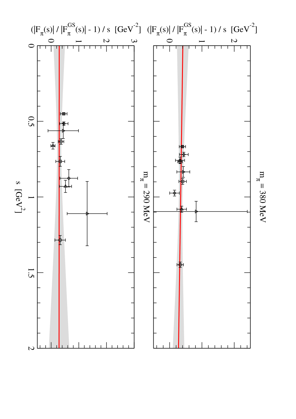
We then use the modified form (13) to describe the lattice data. The difference between the form (8) and (13) can be written as
| (37) |
In Fig. 14 we show the data of as a function of . The data points seem to be well described by a straight line up to statistical fluctuations. We therefore fit them to the form . The fitting results for and , together with determined from charge conservation, are given in Table 3. Within current statistics, the values of are consistent with for both pion masses, and it is not necessary to pursue higher polynomial terms with . Putting , and into (13), we draw the fit curves for in Fig. 13. By including the polynomial terms, the curves match the lattice data. Note that we have imposed the charge conservation condition when obtaining the values of in Table 3. If we do not impose this constraint and fit with a free , we find for at 380 MeV and 1.12(16) at MeV. The charge conservation condition is well reproduced by our lattice data.
As a by-product of this calculation, we evaluate the pion mean-square charge radius (isovector part only) through
| (38) |
using the modified GS form. The first term arises from the GS model with and defined in (45). The second and third terms are the polynomial corrections. The results for are listed in Table 4, where they are compared with the calculation in the spacelike momentum transfer on the same gauge ensembles [56, 57]. The central values of the timelike data seem systematically larger than the spacelike ones but still consistent within the statistical errors.
| Lattice | = “380 MeV” | = “290 MeV” |
|---|---|---|
| (MeV) | ||
| (MeV) | ||
| 5.85(19) | 5.78(23) | |
| (timelike) (fm2) | 0.377(38) | 0.392(41) |
| (spacelike) (fm2) | 0.334(10)() | 0.366(19)() |
VI Conclusion
In this work, we calculate the complex phase and the modulus of the pion form factor in the timelike momentum region. We perform the calculation at two pion masses = 380 MeV and 290 MeV and at a lattice spacing of = 0.11 fm on -flavor overlap fermion configurations generated by the JLQCD Collaboration.
In the elastic scattering region, the complex phase of is given by the -wave pion-pion scattering phase, and thus can be evaluated using the standard Lüscher’s finite-volume formula. We obtain the results at ten different values of from one setup in the center-of-mass frame and four in the moving frames. From the energy dependence of the scattering phase, we extract the coupling constant and the -resonance mass .
Lattice calculation of the modulus of the pion form factor was originally proposed in [27], and here we extend the method to general moving frames and perform the actual calculation using the all-to-all propagator technique. We obtain a clear signal of the form factor and phase indicating the vector meson resonance. The lattice data for are not consistent with the simple GS model. To address this discrepancy we introduce a simple polynomial correction to the GS form, which describes the lattice data quite well.
Though we focus on the calculation of the matrix elements , which can be directly related to , the information hidden in the matrix elements of the -current insertion can also be useful for the study of the resonance properties [58, 59, 60].
As an exploratory study, our work demonstrates the feasibility of calculating the pion form factor in the timelike region using lattice QCD. It is still challenging to make a precise comparison to the experimental data, since we need to calculate the form factor at the physical pion mass, extract many more data points and control the errors both statistically and systematically at the level of experimental precision.
Acknowledgements.
We thank our JLQCD colleagues for many valuable suggestions and encouragement. X.F. would like to thank Professor Norman H. Christ for very helpful discussions. Numerical simulations are performed on Hitachi SR16000 at the High Energy Accelerator Research Organization under the support of its Large Scale Simulation Program (No. 12/13-04 and 13/14-04), as well as on another Hitachi SR16000 at the Yukawa Institute for Theoretical Physics, Kyoto University. This work is supported in part by the Grant-in-Aid of the Japanese Ministry of Education (Grants No. 21674002, No. 25287046, No. 26247043, and No. 26400259), by MEXT SPIRE and JICFuS and by U.S. DOE Grant No. DE-SC0011941.Appendix A Gounaris-Sakurai Model
Using the twice-subtracted dispersion relation, one can relate the real part of to its imaginary part through
| (39) |
where denotes the principal value of the integral. Inserting (11) into the dispersion relation, one has
| (40) |
where the function is given by
| (41) |
for . Using the conditions
| (42) |
one can determine the constants and and find for
| (43) |
This finally results in the GS form factor as
| (44) |
with
| (45) |
Here we use the same notations as in [61].
Using the Watson’s theorem, it is natural to find for the -wave pion-pion scattering phase
| (46) |
Near the resonance energy , one has
| (47) |
This approximation reproduces the effective range formula, which was proposed in [62] and commonly used in previous lattice QCD studies [11, 12, 13, 14, 15, 16, 17] to describe the dependence of the scattering phase. Note that both the GS model and effective range formula account for the leading-order Taylor expansion term at and thus have no control of the dependence for . In [17], various barriers were set for large but with the given statistics different parametrizations are not distinguishable. Considering the fact that the current calculation mainly collects the data near the resonance energy, we simply adopt (46) in our analysis.
Appendix B Lüscher’s formula used in this calculation
Given the total momentum and irreducible representation , the ways to construct the function are given in [41] for the center-of-mass frame and in [42] for the general moving frames. Here we simply give the expressions for , which are defined through
| (48) |
with no ambiguity by setting and requiring a continuous dependence of on . The denominator is given by
| (49) |
In the above expression, is a short-hand notation for the zeta function , which is defined through
| (50) |
with
| (51) |
and
| (52) |
is divergent for and needs to be analytically continued in a numerical calculation. An analytically continued form of is given in [50] and confirmed by [63] with detailed derivations.11 1 In [63], the zeta function is defined using rather than its complex conjugate.
Appendix C Lellouch-Lüscher formula in the -wave scattering
In the infinite volume limit, the correlator turns out to be
In a general moving frame, the center of mass is moving with velocity and the momenta and (center-of-mass momentum) are related to each other by the standard Lorentz transformation
| (54) |
where we have defined
| (55) |
with and . Note that the measure and delta function are Lorentz invariant and satisfy
| (56) |
However, the amplitude is not invariant and transforms as
| (57) | |||||
with for and for .
On the other hand, when taking a large volume limit in (15), the summation over discrete energy states will change to a continuum integral
| (59) |
where we have used the Lüscher’s quantization condition (16). The correlator is now given by
| (60) |
Comparing (60) and (58) we obtain the relation (17). Strictly speaking, the equivalent integral does not mean the equivalent integrand. Also, in the demonstration we have used the Lüscher’s quantization condition, which is only valid in the elastic scattering region. However, the integrals given by (60) and (58) cover also the inelastic scattering region. To make a more rigorous demonstration, one can extend the approach of [27] to the moving frames by requiring that the particle carry the nonzero momentum. This is very similar to the extension of the Lellouch-Lüscher formula [10] to the moving frames [25, 26].
References
- [1] J. J. Dudek and R. G. Edwards, Phys.Rev.Lett. 97, 172001 (2006), hep-ph/0607140.
- [2] S. D. Cohen, H.-W. Lin, J. Dudek, and R. G. Edwards, PoS LATTICE2008, 159 (2008), 0810.5550.
- [3] E. Shintani, S. Aoki, S. Hashimoto, T. Onogi, and N. Yamada, PoS LATTICE2010, 159 (2010), 1102.5544.
- [4] JLQCD Collaboration, X. Feng et al., PoS LATTICE2011, 154 (2011).
- [5] X. Feng et al., Phys.Rev.Lett. 109, 182001 (2012), 1206.1375.
- [6] H.-W. Lin and S. D. Cohen, PoS ConfinementX, 113 (2012), 1302.0874.
- [7] T. Blum et al., Phys.Rev.Lett. 108, 141601 (2012), 1111.1699.
- [8] T. Blum et al., Phys.Rev. D86, 074513 (2012), 1206.5142.
- [9] RBC Collaboration, UKQCD Collaboration, P. Boyle et al., Phys.Rev.Lett. 110, 152001 (2013), 1212.1474.
- [10] L. Lellouch and M. Luscher, Commun.Math.Phys. 219, 31 (2001), hep-lat/0003023.
- [11] CP-PACS Collaboration, S. Aoki et al., Phys.Rev. D76, 094506 (2007), 0708.3705.
- [12] QCDSF Collaboration, M. Gockeler et al., PoS LATTICE2008, 136 (2008), 0810.5337.
- [13] X. Feng, K. Jansen, and D. B. Renner, Phys.Rev. D83, 094505 (2011), 1011.5288.
- [14] C. B. Lang, D. Mohler, S. Prelovsek, and M. Vidmar, Phys.Rev. D84, 054503 (2011), 1105.5636.
- [15] PACS-CS Collaboration, S. Aoki et al., Phys.Rev. D84, 094505 (2011), 1106.5365.
- [16] C. Pelissier and A. Alexandru, Phys.Rev. D87, 014503 (2013), 1211.0092.
- [17] J. J. Dudek, R. G. Edwards, and C. E. Thomas, Phys.Rev. D87, 034505 (2013), 1212.0830.
- [18] QCDSF/UKQCD Collaboration, D. Brommel et al., Eur.Phys.J. C51, 335 (2007), hep-lat/0608021.
- [19] ETM Collaboration, R. Frezzotti, V. Lubicz, and S. Simula, Phys.Rev. D79, 074506 (2009), 0812.4042.
- [20] P. Boyle et al., JHEP 0807, 112 (2008), 0804.3971.
- [21] JLQCD Collaboration, TWQCD Collaboration, S. Aoki et al., Phys.Rev. D80, 034508 (2009), 0905.2465.
- [22] O. H. Nguyen, K.-I. Ishikawa, A. Ukawa, and N. Ukita, JHEP 1104, 122 (2011), 1102.3652.
- [23] B. B. Brandt, A. Juttner, and H. Wittig, (2013), 1306.2916.
- [24] J. Koponen, F. Bursa, C. Davies, G. Donald, and R. Dowdall, PoS LATTICE2013, 282 (2014), 1311.3513.
- [25] N. H. Christ, C. Kim, and T. Yamazaki, Phys.Rev. D72, 114506 (2005), hep-lat/0507009.
- [26] C. Kim, C. Sachrajda, and S. R. Sharpe, Nucl.Phys. B727, 218 (2005), hep-lat/0507006.
- [27] H. B. Meyer, Phys.Rev.Lett. 107, 072002 (2011), 1105.1892.
- [28] G. Gounaris and J. Sakurai, Phys.Rev.Lett. 21, 244 (1968).
- [29] S. Protopopescu et al., Phys.Rev. D7, 1279 (1973).
- [30] P. Estabrooks and A. D. Martin, Nucl.Phys. B79, 301 (1974).
- [31] R. Akhmetshin et al., JETP Lett. 84, 413 (2006), hep-ex/0610016.
- [32] CMD-2 Collaboration, R. Akhmetshin et al., Phys.Lett. B648, 28 (2007), hep-ex/0610021.
- [33] M. Achasov et al., J.Exp.Theor.Phys. 103, 380 (2006), hep-ex/0605013.
- [34] KLOE Collaboration, F. Ambrosino et al., Phys.Lett. B700, 102 (2011), 1006.5313.
- [35] Particle Data Group, J. Beringer et al., Phys.Rev. D86, 010001 (2012).
- [36] F. Jegerlehner and R. Szafron, Eur.Phys.J. C71, 1632 (2011), 1101.2872.
- [37] ALEPH Collaboration, S. Schael et al., Phys.Rept. 421, 191 (2005), hep-ex/0506072.
- [38] M. Davier, A. Hocker, and Z. Zhang, Rev.Mod.Phys. 78, 1043 (2006), hep-ph/0507078.
- [39] D. Melikhov, O. Nachtmann, and T. Paulus, (2002), hep-ph/0209151.
- [40] C. Bruch, A. Khodjamirian, and J. H. Kuhn, Eur.Phys.J. C39, 41 (2005), hep-ph/0409080.
- [41] M. Luscher, Nucl.Phys. B354, 531 (1991).
- [42] K. Rummukainen and S. A. Gottlieb, Nucl.Phys. B450, 397 (1995), hep-lat/9503028.
- [43] C. D. Lin, G. Martinelli, C. T. Sachrajda, and M. Testa, Nucl.Phys. B619, 467 (2001), hep-lat/0104006.
- [44] S. Aoki et al., PTEP 2012, 01A106 (2012).
- [45] JLQCD Collaboration, H. Fukaya et al., Phys.Rev. D74, 094505 (2006), hep-lat/0607020.
- [46] S. Aoki, H. Fukaya, S. Hashimoto, and T. Onogi, Phys.Rev. D76, 054508 (2007), 0707.0396.
- [47] J. Noaki et al., Phys.Rev. D81, 034502 (2010), 0907.2751.
- [48] J. Foley et al., Comput.Phys.Commun. 172, 145 (2005), hep-lat/0505023.
- [49] Q. Liu, PoS LATTICE2011, 287 (2011), 1110.2143.
- [50] ETM Collaboration, X. Feng, K. Jansen, and D. B. Renner, PoS LATTICE2010, 104 (2010), 1104.0058.
- [51] M. Luscher and U. Wolff, Nucl.Phys. B339, 222 (1990).
- [52] SESAM Collaboration, G. S. Bali, H. Neff, T. Dussel, T. Lippert, and K. Schilling, Phys.Rev. D71, 114513 (2005), hep-lat/0505012.
- [53] X. Feng, K. Jansen, and D. B. Renner, Phys.Lett. B684, 268 (2010), 0909.3255.
- [54] T. Blum et al., Phys.Rev. D84, 114503 (2011), 1106.2714.
- [55] J. J. Dudek, R. G. Edwards, and C. E. Thomas, Phys.Rev. D86, 034031 (2012), 1203.6041.
- [56] JLQCD Collaboration, T. Kaneko et al., PoS LATTICE2010, 146 (2010), 1012.0137.
- [57] H. Fukaya et al., Phys.Rev. D90, 034506 (2014), 1405.4077.
- [58] G. Meng and C. Liu, Phys.Rev. D78, 074506 (2008), 0804.4308.
- [59] Z.-Y. Niu, M. Gong, C. Liu, and Y. Shen, Phys.Rev. D80, 114509 (2009), 0909.3154.
- [60] Z.-Y. Niu et al., Phys.Rev. D82, 054501 (2010), 1005.5571.
- [61] A. Francis, B. Jager, H. B. Meyer, and H. Wittig, Phys.Rev. D88, 054502 (2013), 1306.2532.
- [62] M. Luscher, Nucl.Phys. B364, 237 (1991).
- [63] L. Leskovec and S. Prelovsek, Phys.Rev. D85, 114507 (2012), 1202.2145.