Numerical pricing of American options under two stochastic factor models with jumps using a meshless local Petrov-Galerkin method

Journal: .

Jamal Amani Rad Email: j.amanirad@gmail.com;j_amanirad@sbu.ac.ir Kourosh Parand Email: k_parand@sbu.ac.ir Address: Department of Computer Sciences, Faculty of Mathematical Sciences, Shahid Beheshti University, Evin, P.O. Box 198396-3113,Tehran,Iran Corresponding author: Corresponding author

Abstract

The most recent update of financial option models is American options under stochastic volatility models with jumps in returns (SVJ) and stochastic volatility models with jumps in returns and volatility (SVCJ). To evaluate these options, mesh-based methods are applied in a number of papers but it is well-known that these methods depend strongly on the mesh properties which is the major disadvantage of them. Therefore, we propose the use of the meshless methods to solve the aforementioned options models, especially in this work we select and analyze one scheme of them, named local radial point interpolation (LRPI) based on Wendland’s compactly supported radial basis functions (WCS-RBFs) with $C^{6}$ , $C^{4}$ and $C^{2}$ smoothness degrees. The LRPI method which is a special type of meshless local Petrov-Galerkin method (MLPG), offers several advantages over the mesh-based methods, nevertheless it has never been applied to option pricing, at least to the very best of our knowledge. These schemes are the truly meshless methods, because, a traditional non-overlapping continuous mesh is not required, neither for the construction of the shape functions, nor for the integration of the local sub-domains. In this work, the American option which is a free boundary problem, is reduced to a problem with fixed boundary using a Richardson extrapolation technique. Then the implicit-explicit (IMEX) time stepping scheme is employed for the time derivative which allows us to smooth the discontinuities of the options’ payoffs. Stability analysis of the method is analyzed and performed. In fact, according to an analysis carried out in the present paper, the proposed method is unconditionally stable. Numerical experiments are presented showing that the proposed approaches are extremely accurate and fast.

Keywords:

Option Pricing, Stochastic volatility, European option, American option, Merton jump-diffusion, SV model, SVJ model, SVCJ model, Meshless weak form, LRPI, MLPG, Wendland functions, Richardson extrapolation, Stability analysis.
AMS subject classification: 91G80; 91G60; 35R35.

1 Introduction

In the field of numerical methods, the finite element method (FEM) and other mesh-based methods such as finite difference method (FDM) and finite volume method (FVM) are robust and well established. Therefore, they are widely used in financial field due to their applicability to many types of options, see [1, 2, 3, 4]. In the FEM, a computational domain is divided into finite elements which are connected together called a mesh. Although the FEM and the closely related FVM are well-established numerical techniques for computer modeling in engineering and sciences, they are not without shortcoming. It is well-known that these methods depend strongly on the mesh properties. However, to compute problems with irregular geometries using these schemes, mesh generation is a far more time consuming and expensive task than solution of the PDEs [5].

To overcome this difficulty associated with FEM and FVM, the boundary element method (BEM) [6] appears to be a attractive alternative. In the BEM, only the boundary of domain needs to be discretized [7, 8, 9, 10]. This reduces the problem dimension by one and thus largely reduces the time in meshing. The BEM still uses elements to implement both interpolation and integration [7, 8, 9, 10].

These difficulties can be overcome by the meshless methods (MLM), which have attracted considerable interest over the past decade. MLM also known as meshfree methods. The main advantage of these methods is to approximate the unknown field by a linear combination of shape functions built without having recourse to a mesh of the domain. In this method, we use a set of nodes scattered within the domain of the problem as well as sets of nodes on the boundaries of the domain to represent (not discretize) the domain of the problem and its boundaries [11]. These sets of scattered nodes are called field nodes and they do not form a mesh, meaning it does not require any priori information on the relation ship between the nodes for the interpolation or approximation of the unknown functions of field variables [12].

Meshless methods have progressed remarkably in the last decades and some work has been devoted to their classification. The classification can be done based on different criteria, e.g., formulation procedure, shape function or the domain representation [13]. The formulation procedures are mainly based on the weak from representation (see [14, 15, 16, 17, 18]) and the strong form based on the collocation techniques (see [19, 20, 21, 22]), although a combination of both approaches is possible [23]. The collocation methods are truly meshless, as the collocation technique is directly based on a set of nodes without any background mesh for numerical integration. One limitation of the collocation methods is less accuracy and lower stability in numerical implementation. However, this method is based on point collocation, and is very sensitive to the choice of collocation points, see [24, 25]. On the other hands, the weak forms are used to derive a set of algebraic equations through a numerical integration process using a set of quadrature domain that may be constructed globally or locally in the domain of the problem, such as the element-free Galerkin method (EFG) [26], the reproducing kernel particle method (RKPM) [27] and the partition unity method (PUM) [28]. The above-mentioned methods are all based on a global weak form, being meshless only in terms of the interpolation of the field or boundary variables, and have to use background cells to integrate over the problem domain. The requirement of background cells for integration makes these methods being not truly meshless. In order to alleviate the global integration background cells, the meshless local Petrov-Galerkin method (MLPG) based on local weak-form and the radial basis functions (RBFs) approximation, was developed by Atluri and his colleagues [29]. This method also known as local radial point interpolation (LRPI) method. The MLPG method is a truly meshless method, because, a traditional non-overlapping, continuous mesh is not required, either for the construction of the shape function, or for the integration of the local sub-domain. The trial and test function spaces can be different or the same. It offers a lot of flexibility to deal with different boundary value problems. A wide range of problems has been solved by Atluri and his coauthors [23, 30]. In this type of MLPG method, the Heaviside step function is employed as a test function. Particularly, the LRPI meshless method reduces the problem dimension by one, has shape functions with delta function properties, and expresses the derivatives of shape functions explicitly and readily. Thus it allows one to easily impose essential boundary and initial (or final) conditions. For some works on the meshless local method one can mention the works of Sladek brothers [31, 32, 33, 34, 35]. The method has now been successfully extended to a wide rang of problems in engineering. For some examples of these problems, see [11, 36] and other references therein. The interested reader of meshless methods can also see [14, 15, 16].

Over the last years, the growth of the financial markets has been an ever expanding economical field. In all over the world, the value of the financial assets traded on the stock markets has reached astronomical amounts. Trading of financial derivatives such as options is a continuous business going on all over the world. Making sure that the price are correct at every time is of great importance for the traders.
Options are financial contracts that gives to the buyer the right, to buy (call option) or to sell (put option) an underlying asset (such as a stock) at a previous agreed price. Called the strike or exercise price on or before a certain time called the maturity. Mast of these options can be grouped into either of the two categories: European options which can only be exercised at one given expiry or maturity date ( $t=T$ ) and American options can additionally be executed at any time prior to their maturity date ( $t\leq T$ ). The American options give the freedom when to use the option and are often a little bit more expensive than a corresponding European options.
The valuation of options lead to mathematical models that are often challenging to solve. The famous Black-Scholes formula gives an explicit pricing formula for European call and put options on stocks which do not pay dividends, see [37]. The publication in 1973 [38] of the work of Fischer Black and Myron Scholes has been a starting point for the revolution in the option pricing. Their idea was to develop a model based on the assumption that the asset prices follow a geometric Brownian motion. For European options the Black-Scholes equation results in a boundary value problem of a diffusion equation. American options pricing is governed by a parabolic partial differential variational inequality (PDVI). This gives rise to a free boundary problem, see [39, 40].

Recently, by using very empirical studies, it has become evident that the assumption of behavior like a log-normal strike diffusion with a constant volatility and a drift in the standard Black-Scholes model of the underlying asset price is not consistent with that the real market prices of options with various strike prices and maturities such as volatility smile or skew and heavy tails [41, 42].

During the last decade, many works have been done to find modifications of classical Black-Scholes model to satisfy these phenomena in financial markets such as the models with stochastic volatility (SV), the models with jumps (such as Merton and Kou models proposed by Merton and Kou in two different works [43] and [44], respectively), their combinations of stochastic volatility and jumps in returns, i.e. stochastic volatility models with jumps (SVJ) introduced by Bates [45], and stochastic volatility models with jumps in returns and volatility (SVCJ) introduced by Duffie et al. [46].

In this research, we focus on the SVJ and SVCJ models. In this work, Merton model is selected to jump term of model. In Merton’s model the asset return follows a standard Wiener process driven by a compound Poisson process with normally distributed jump [42].

We have just mentioned such that the mentioned models of course will also lead to such a volatility smile or skews on short or long term maturity ranges [3].

The mentioned SVJ and SVCJ models for pricing American options are governed by a parabolic integro-differential variational inequality which can be formulated as a free boundary problem. In particular, these models are contain differential term and a nonlocal integral term. Hence, an analytical solution is impossible. Therefore, to solve these problems, we need to have a powerful computational method. To this aim, several numerical methods have been proposed for pricing options under SVJ and SVCJ models (see, e.g., [3, 47, 48, 49]) but weak form meshless methods have never been used for option pricing of this model, at least to the very best of our knowledge.

The objective of this paper is to extend the LRPI based on Wendland’s compactly supported radial basis functions (WCS-RBFs) with $C^{6}$ , $C^{4}$ and $C^{2}$ smoothness [50] to evaluate American options under SVJ and SVCJ models. Again we do emphasize that, to the best of our knowledge, the local weak form of meshless method has not yet been used in mathematical finance. Therefore, it appears to be interesting to extend such a numerical technique also to option valuation, which is done in the presented manuscript.

In addition, in this paper the infinite space domain $\mathbb{R}^{+}\times\mathbb{R}^{+}$ is truncated to $[0,S_{max}]\times[0,y_{max}]$ in SVJ and SVCJ models, with the sufficiently large values $S_{max}$ and $y_{max}$ to avoid an unacceptably large truncation error. The options’ payoffs considered in this paper are non-smooth functions, in particular their derivatives are discontinuous at the strike price. Therefore, to reduce as much as possible the losses of accuracy the points of the trial functions are concentrated in a spatial region close to the strike prices. So, we employ the change of variables proposed by Clarke and Parrott [51].

As far as the time discretization is concerned, we use the implicit-explicit (IMEX) time stepping scheme, which is unconditionally stable and allows us to smooth the discontinuities of the options’ payoffs. Note that in SVJ and SVCJ models, the integral part is a non-local integral, whereas the other parts which are differential operators, are all local. No doubt, since the integral part is non-local operator, a dense linear system of equations will be obtained by using the $\theta$ -weighted discretization scheme. Therefore, to obtain a sparse linear system of equations, it is better to use a IMEX scheme which is noted for avoiding dense matrices. So far, and to the best of knowledge, published work existing in the literature which use the IMEX scheme to price the options, include [3, 47]. Such an approach is only first-order accurate, however a second-order time discretization is obtained by performing a Richardson extrapolation procedure with halved time step. Stability analysis of the method is analyzed and performed by the matrix method in the present paper.

Finally, in order to solve the free boundary problem that arises in the case of American options is computed by Richardson extrapolation of the price of Bermudan option. In essence the Richardson extrapolation reduces the free boundary problem and linear complementarity problem to a fixed boundary problem which is much simpler to solve.

Numerical experiments are presented showing that the proposed approach is very efficient from the computational standpoint. In particular, the prices of both European and American options in SVJ or SVCJ models can be computed with an error (in both the maximum norm and the root mean square relative difference) of order $10^{-3}$ in few tenth of a second. Moreover, the Bermudan approximation reveals to be the most efficient of the algorithms used to deal with the early exercise opportunity.

We remark that the main contribution of this manuscript is to show that the MLPG, which, to the best of our knowledge, has never been applied to problems in mathematical finance, can yield accurate and fast approximations of European and American option prices.

Overall , our focus in this paper is more devoted to providing an accurate, computationally fast, stable, convergence and simple technique for pricing options under SVJ and SVCJ models. We should note that the key idea of this work is finding a new technique combined using the following numerical tools : Spatial change of variables, time discretization of the Black-Scholes operator, Richardson extrapolation procedure, LRPI discretization, Wendland’s compactly supported radial basis functions, Spatial variable transformation , approximate the price of the American option with the price of a Bermudan option and LU factorization method with partial pivoting. Rigorously speaking, these tools considered separately, are not new, but here due to the fact that an approach that puts all these techniques together has never been proposed in option pricing, therefore the proposed technique is new, accurate and very fast.

The paper is organized as follows: In Section 2 a detailed description of the SVJ and SVCJ models for American options is provided. Section 3 is devoted to presenting the MLPG approach and the application of such a numerical technique to the option pricing problems considered is shown in this section. The numerical results obtained are presented and discussed in Section 4 and finally, in Section 5, some conclusions are drawn.

2 The option pricing models

2.1 SVJ or Bates SV model

For the sake of simplicity, from now we restrict our attention to options of call type, but the case of put options can be treated in perfect analogy.

First we are interested in pricing a American call option of the Bates stochastic volatility model which is the exponential L $\acute{e}$ vy processes consisting of a two-dimensional geometric Brownian motion plus a compound Possion jumps with time varying volatility.

Let $(\Omega,\mathcal{F},\mathbf{P})$ be a probability space and also $X_{t}$ be a continues L $\acute{e}$ vy process with a L $\acute{e}$ vy measure $\nu$ . In the Bates model which is an arbitrage-free market model, the asset price $S_{t}$ with time $t\in[0,T]$ and $T$ being the maturity time is than given by

\displaystyle S_{t}=S_{0}e^{X_{t}},

where $S_{0}$ is the asset price at time zero.

Then the risk-neutral dynamics of the asset price $S_{t}$ and its volatility $Y_{t}$ are described by the following stochastic differential equations [3, 48, 49]

	$\displaystyle\frac{dS_{t}}{S_{t}}=\alpha~dt+\sqrt{Y_{t}}~dW_{t}^{1}+dJ_{t},$
	$\displaystyle dY_{t}=\xi(\eta-Y_{t})~dt+\theta\sqrt{Y_{t}}~dW_{t}^{2},$

where $(W_{t}^{1},W_{t}^{2})$ are two Brownian motions with correlation factor $\rho\in[-1,1]$ , $\xi,\eta,\theta\in\mathbb{R}^{+}$ are mean-reversion rate, long-run mean and the instantaneous volatility of $Y_{t}$ , respectively, $J_{t}=\sum_{j=1}^{N_{t}}R_{j}$ is a compound Poisson process, where $N_{t}$ is a Possion process with intensity $\lambda$ and the set ${R_{j}}$ is a sequence of independent and identically distributed (i.i.d.) random variables with density $\nu(dx)/\lambda$ . Also $\alpha=r-q-\lambda\kappa$ is the drift rate, where $r$ is the risk-free interest rate, $q$ is the dividend and $\kappa$ is the expected relative jump size. Here, we can rewrite the L $\acute{e}$ vy measure $\nu(dx)$ as $\lambda f(x)dx$ where $f(x)$ is a weight function. By selecting this weight function the finite activity jump-diffusion model is the log-normal model proposed by Merton [43]

\displaystyle f(x)=\frac{1}{\sqrt{2\pi}x\delta}\exp(-\frac{(\log x-\gamma)^{2}}{2\delta^{2}}),

(2.1)

Note that $f(x)\geq 0$ and

\displaystyle\int_{\mathbb{R}^{+}}f(x)dx=1.

(2.2)

We now consider the pricing of an American call option denoted by $V(s,y,t)$ on the underlying asset $S_{t}$ with asset price $E$ and maturity $T$ . On can show that $V(s,y,t)$ , for $s,y\in[0,+\infty)$ and $t\in[0,T)$ , satisfy the following system of free boundary problem

	$\displaystyle\frac{\partial}{\partial t}V(s,y,t)+\mathcal{L}V(s,y,t)=0~,~~~~~~~~~~~~~~~~~~~~~0\leq s<B(y,t)~,$		(2.3)
	$\displaystyle V(s,y,t)=s-E~,~~~~~~~~~~~~~~~~~~~~~~~~~~~~s>B(y,t)~,$		(2.4)
	$\displaystyle\lim_{s\rightarrow B(y,t)}\frac{\partial V(s,y,t)}{\partial s}=1~,$		(2.5)
	$\displaystyle\lim_{s\rightarrow B(y,t)}\frac{\partial V(s,y,t)}{\partial y}=0~,$		(2.6)

where

	$\displaystyle\mathcal{L}V(s,y,t)=-\mathbf{F}\times\nabla V(s,y,t)+\nabla.(\mathbf{E}\times\nabla V(s,y,t))-(r+\lambda)V(s,y,t)+\lambda\int_{\mathbb{R}^{+}}V(sx,y,t)f(x)dx,$
			(2.7)

	$\displaystyle\mathbf{E}=\frac{1}{2}\left(\begin{array}[]{cc}ys^{2}&\rho\theta sy\\ \rho\theta sy&\theta^{2}y\end{array}\right)~,$
	$\displaystyle\mathbf{F}=-\left(\begin{array}[]{c}(r-q-\lambda\kappa)s-ys-\rho\frac{\theta}{2}s\\ \xi(\eta-y)-\frac{\theta^{2}}{2}-\rho\frac{\theta}{2}y\end{array}\right)^{T}~.$

Again we should note that $\kappa$ is the expected relative jump size and is computed as $\kappa=\int_{\mathbb{R}^{+}}(z-1)f(z)dz$ . We have $\kappa=\exp(\gamma+\delta^{2}/2)-1$ for Merton model.

The value of $V$ at maturity is given by

\displaystyle V(s,y,T)=\varsigma(s)~,

(2.14)

where $\varsigma$ is the so-called option’s payoff:

\displaystyle\varsigma(s)=\mathrm{max}(s-E,0)~,

(2.15)

which is clearly not differentiable at $s=E$ .

The behavior of the value of the American call option on the boundaries is given by

\displaystyle V(0,y,t)=0~,~~~~~~\lim_{s\rightarrow+\infty}V(s,y,t)=s-E~~.

(2.16)

In relations (2.3)-(2.6), $B(y,t)$ denotes the so-called exercise boundary, which is unknown and is implicitly defined by (2.3)-(2.16). The above free-boundary partial differential problem does not have an exact closed-form solution, and thus some numerical approximation is required.

Problem (2.3)-(2.16) can be reformulated as a linear complementarity problem:

	$\displaystyle\frac{\partial}{\partial t}V(s,y,t)+\mathcal{L}V(s,y,t)\geq 0~,$		(2.17)
	$\displaystyle V(s,y,t)-\varsigma(s)\geq 0~,$		(2.18)
	$\displaystyle\left(\frac{\partial}{\partial t}V(s,y,t)+\mathcal{L}V(s,y,t)\right)\cdot\left(V(s,y,t)-\varsigma(s)\right)=0~,$		(2.19)

which holds for $s,y\in(0,+\infty)$ and $t\in[0,T)$ , with final condition:

\displaystyle V(s,y,T)=\varsigma(s)~,

(2.20)

and boundary conditions:

\displaystyle V(0,y,t)=0~,~~~~~~\lim_{s\rightarrow+\infty}V(s,y,t)=s-E~~.

(2.21)

2.2 SVCJ model

In the Bates models, Poisson jumps are only added to the risk-neutral dynamic of the asset price $S_{t}$ . In contrast, in the SVCJ models, jumps are appeared in the volatility, too. Then we have [47]

	$\displaystyle\frac{dS_{t}}{S_{t}}=\alpha_{s}~dt+\sqrt{Y_{t}}~dW_{t}^{1}+dJ^{1}_{t},$		(2.22)
	$\displaystyle dY_{t}=\xi(\eta-Y_{t})~dt+\theta\sqrt{Y_{t}}~dW_{t}^{2}+dJ^{2}_{t},$		(2.23)

where $\alpha_{s}=r-q-\lambda\kappa_{s}$ such that $\kappa_{s}=(1-\nu\rho_{j})^{-1}\exp(\gamma+\delta^{2}/2)-1$ and $\rho_{j}$ defines the correlation between jumps in returns and variance. The two-dimensional jump process $(J^{1},J^{2})$ is a $\mathbb{R}\times\mathbb{R}^{+}$ -valued compound Poisson process with intensity $\lambda$ [47]. The distribution of the jump size in variance is assumed to be exponential with mean $\nu$ . Conditional on a jump of size $z^{v}$ in the variance process, $J^{1}+1$ has a log-normal distribution $f(z^{s},z^{v})$ with the mean in log $z^{s}$ being $\gamma+\rho_{j}z^{v}$ [47]. This gives a bivariate probability density function defined by [47]

f(z^{s},z^{v})=\frac{1}{\sqrt{2\pi}z^{s}\delta\nu}\exp\Bigg(-\frac{z^{v}}{\nu}-\frac{(\log z^{s}-\gamma-\rho_{j}z^{v})^{2}}{2\delta^{2}}\Bigg).

Let $V(s,y,t)$ denote the price of a American derivative on an underlying asset described by model 2.22 and 2.23. As in [47], it can be shown that $V(s,y,t)$ is governed by the partial integro-differential equation

	$\displaystyle\frac{\partial}{\partial t}V(s,y,t)+\mathcal{L}V(s,y,t)=0~,~~~~~~~~~~~~~~~~~~~~~0\leq s<B(y,t)~,$		(2.24)
	$\displaystyle V(s,y,t)=s-E~,~~~~~~~~~~~~~~~~~~~~~~~~~~~~s>B(y,t)~,$		(2.25)
	$\displaystyle\lim_{s\rightarrow B(y,t)}\frac{\partial V(s,y,t)}{\partial s}=1~,$		(2.26)
	$\displaystyle\lim_{s\rightarrow B(y,t)}\frac{\partial V(s,y,t)}{\partial y}=0~,$		(2.27)

where

	$\displaystyle\mathcal{L}V(s,y,t)=-\mathbf{F}\times\nabla V(s,y,t)+\nabla.(\mathbf{E}\times\nabla V(s,y,t))-(r+\lambda)V(s,y,t)$
	$\displaystyle+\lambda\int_{\mathbb{R}^{+}}\int_{\mathbb{R}^{+}}V(sz^{s},y+z^{v},t)f(z^{s},z^{v})dz^{v}~dz^{s},$
			(2.28)

	$\displaystyle\mathbf{E}=\frac{1}{2}\left(\begin{array}[]{cc}ys^{2}&\rho\theta sy\\ \rho\theta sy&\theta^{2}y\end{array}\right)~,$
	$\displaystyle\mathbf{F}=-\left(\begin{array}[]{c}(r-q-\lambda\kappa)s-ys-\rho\frac{\theta}{2}s\\ \xi(\eta-y)-\frac{\theta^{2}}{2}-\rho\frac{\theta}{2}y\end{array}\right)^{T}~,$

the final and boundary conditions for this model are described in relations (2.20) and (2.21).

3 Methodology

In this work, the price of American option is computed by Richardson extrapolation of the price of Bermudan option. In essence the Richardson extrapolation reduces the free boundary problem and linear complementarity problem to a fixed boundary problem which is much simpler to solve. Thus, instead of describing the aforementioned linear complementarity problem or penalty method, we directly focus our attention onto the partial integro-differential equation satisfied by the price of a Bermudan option which is faster and more accurate than other methods.

For the sake of simplicity exposition, we restrict our attention to option of the Bates stochastic volatility model, but the case of options under SVCJ model can be treated in perfect analogy.

Let us consider in the interval $[0,T]$ , $M+1$ equally spaced time levels $t_{0}=0,t_{1},t_{2},...,t_{M}=T$ . Let $V_{M}(s,y,t)$ denote the price of a Bermudan option with maturity $T$ and strike price $E$ . The Bermudan option is an option that can be exercised not on the whole time interval $[0,T]$ , but only at the dates $t_{0}$ , $t_{1}$ , $\ldots$ , $t_{M}$ . That is we consider the problems

\displaystyle\begin{cases}\frac{\partial}{\partial t}V_{M}(s,y,t)+\mathcal{L}V_{M}(s,y,t)=0~,\\ V_{M}(0,y,t)=0~,~~~~~~\lim_{s\rightarrow+\infty}V_{M}(s,y,t)=s-E~.\end{cases}

(3.1)

which hold in the time intervals $(t_{0},t_{1})$ , $(t_{1},t_{2})$ , $\ldots$ , $(t_{M-1},t_{M})$ . By doing that also the relation (2.19) is automatically satisfied in every time interval $(t_{k},t_{k+1})$ , $k=0,1,\ldots,M-1$ . Moreover, the relation (2.18) is enforced only at times $t_{0}$ , $t_{1}$ , $\ldots$ , $t_{M-1}$ , by setting

\displaystyle V_{M}(s,y,t_{k})=\max(\lim_{t\rightarrow t_{k}^{+}}V_{M}(s,y,t),\varsigma(s))~,~~~~~k=0,1,\ldots,M-1.~

(3.2)

Note that the function $V_{M}(\cdot,\cdot,t_{k})$ computed according to (3.2) is used as the final condition for the problem (3.1) that holds in the time interval $(t_{k-1},t_{k})$ , $k=1,2,\ldots,M-1$ . Instead, the final condition for the problem (3.1) that holds in the time interval $(t_{M-1},t_{M})$ , according to the relation (2.20), is prescribed as follows:

\displaystyle V_{M}(s,y,t_{M})=\varsigma(s)~.

(3.3)

That is, in summary, problems (3.1) are recursively solved for $k=M-1,M-2,\ldots,0$ , starting from the condition (3.3), and at each time $t_{M-1}$ , $t_{M-2}$ , $\ldots$ , $t_{0}$ the American constraint (3.2) is imposed.

The Bermudan option price $V_{M}(s,y,t)$ tends to become a fair approximation of the American option price $V(s,y,t)$ as the number of exercise dates $M$ increases. In this work the accuracy of $V_{M}(s,y,t)$ is enhanced by Richardson extrapolation which is second-order accurate in time.

To evaluate the option, the meshless local Petrov-Galerkin (MLPG) method is used in this work. This method is based on local weak forms over intersecting sub-domains, which are extracted over the local sub-domains using divergence theorem and a Heaviside test function. At first we discuss a time-stepping method for the time derivative.

3.1 Time discretization

First of all, we discretize the operator (2.7) in time. For this propose, we can apply the Laplace transform or use a time-stepping approximation. Algorithms for the numerical inversion of a Laplace transform lead to a reduction in accuracy. Then, we employ a time-stepping method to overcome the time derivatives in this operator.

Let $V^{k}(s,y)$ denote a function approximating $V_{M}(s,y,t_{k}),k=0,1,...,M-1$ . Note that the subscript $M$ has been removed from $V^{k}(s,y)$ to keep the notation simple. According to (3.3), we set $V^{M}(s,y)=\varsigma(s)$ . Let us consider the following implicit-explicit (IMEX) time stepping scheme:

\displaystyle\mathcal{L}V^{k}(s,y)=-\mathbf{F}\times\nabla V^{k}(s,y)+\nabla.(\mathbf{E}\times\nabla V^{k}(s,y))-(r+\lambda)V^{k}(s,y)+\lambda\int_{\mathbb{R}^{+}}V^{k+1}(sx,y)f(x)dx,

(3.4)

and also we use

\displaystyle\frac{\partial}{\partial t}V(s,y,t)\simeq\frac{V^{k+1}(s,y)-V^{k}(s,y)}{\Delta t}+\mathcal{O}(\Delta t),

(3.5)

using relations (3.4) and (3.5), we define the following operator

	$\displaystyle\mathcal{\widetilde{L}}V^{k}(s,y)\simeq\frac{V^{k+1}(s,y)-V^{k}(s,y)}{\Delta t}+\mathcal{L}V^{k}(s,y)$
	$\displaystyle=\frac{1}{\Delta t}V^{k+1}(s,y)-\mathbf{F}\times\nabla V^{k}(s,y)+\nabla.(\mathbf{E}\times\nabla V^{k}(s,y))-(r+\lambda+\frac{1}{\Delta t})V^{k}(s,y)+\lambda\int_{\mathbb{R}^{+}}V^{k+1}(sx,y)f(x)dx,$

Therefore, the American option problems are rewritten as follows:

\displaystyle\begin{cases}\mathcal{\widetilde{L}}V^{k}(s,y)=0~,\\ V^{k}(0,y)=0~,~~~~~~\lim_{s\rightarrow+\infty}V^{k}(s,y)=s-E~~.\end{cases}

(3.6)

and also, the relations (3.2) and (3.3) are rewritten as follows:

	$\displaystyle V^{k}(s,y)=\max(\lim_{t\rightarrow t_{k+1}^{+}}V^{k}(s,y),\varsigma(s))~,~~~~~k=M-1,M-2,\ldots,1,0~$		(3.7)
	$\displaystyle V^{M}(s,y)=\varsigma(s)~.$

Remark 1: Note that in relation (3.4), the integral part is a non-local integral, whereas the other parts which are differential operators, are all local. No doubt, since the integral part is non-local operator, a dense linear system of equations will be obtained by using the $\theta$ -weighted discretization scheme. Therefore, to obtain a sparse linear system of equations, it is better to use a IMEX scheme which is noted for avoiding dense matrices. So far, and to the best of knowledge, published work existing in the literature which use the IMEX scheme to price the options, include [47]. Therefore, in this work, we use the IMEX scheme which is only first-order accurate in time. Then, the obtained approximation, which is only first-order accurate, is improved by Richardson extrapolation. In particular, we manage to obtain second-order accuracy by extrapolation of two solutions computed using $M$ and $2M$ time steps. In the following, for the sake of brevity, we will restrict our attention to first stage of the Richardson extrapolation procedure, where $M$ time steps are employed, and the fact that the partial integro-differential problems considered are also solved with $2M$ time steps will be understood.

3.2 Spatial variable transformation

It is well-known that from the mathematical point of view, the Bates stochastic volatility model typically leads to a partial integro-differential equation that is defined in the unbounded spatial domain $\mathbb{R}^{+}\times\mathbb{R}^{+}$ . But due to the fact that it requires large memory storage, we replace the domain with the finite domain $\Omega=[0,S_{max}]\times[0,y_{max}]$ of the asset price and the volatility, where $S_{max}$ and $y_{max}$ are chosen sufficiently large to avoid an unacceptably large truncation error. However, in [52] shown that upper bound of the asset price is three or four times of the strike price, so we can set $S_{max}=4E$ . The options’ payoffs considered in this paper are non-smooth functions, in particular their derivatives are discontinuous at the strike price. Therefore, to reduce the losses of accuracy the points of the trial functions are concentrated in a spatial region close to $s=E$ . In contrast, along the $y$ -direction, we want to have a mesh which is finer in a neighborhood of $y=y_{0}$ , where the possible realizations of the variance process are more likely to occur [3]. So, we employ the following change of variables:

	$\displaystyle x(s)=\frac{\sinh^{-1}(\xi_{s}(s-E))+\sinh^{-1}(\xi_{s}E)}{\sinh^{-1}(\xi_{s}(S_{max}-E))+\sinh^{-1}(\xi_{s}E)},$		(3.8)
	$\displaystyle z(y)=\frac{\sinh^{-1}(\xi_{y}(y-y_{0}))+\sinh^{-1}(\xi_{y}y_{0})}{\sinh^{-1}(\xi_{y}(y_{max}-y_{0}))+\sinh^{-1}(\xi_{y}y_{0})},$		(3.9)

	$\displaystyle s(x)=\frac{1}{\xi_{s}}\sinh\Bigg(x\sinh^{-1}(\xi_{s}(S_{max}-E))-(1-x)\sinh^{-1}(\xi_{s}E)\Bigg)+E,$		(3.10)
	$\displaystyle y(z)=\frac{1}{\xi_{y}}\sinh\Bigg(z\sinh^{-1}(\xi_{y}(y_{max}-y_{0}))-(1-z)\sinh^{-1}(\xi_{y}y_{0})\Bigg)+y_{0},$

where $\xi_{s}$ and $\xi_{y}$ are the suitable constant parameters. Using these parameters, we can control the amount of the distribution of nodes in the $s$ and $y$ -directions near $s=E$ and $y=y_{0}$ , see Figure 1.

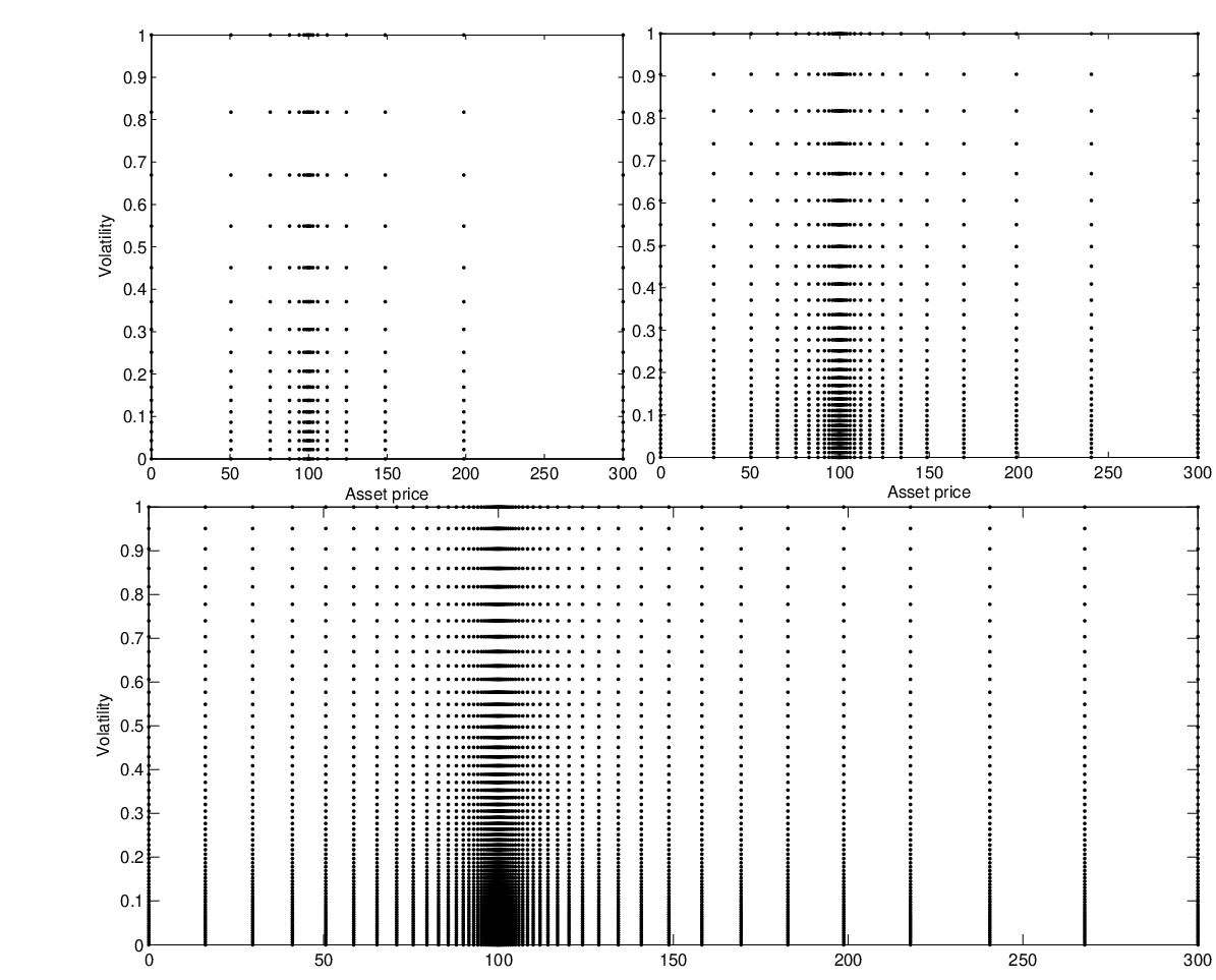
Refer to caption — Figure 1: $\xi_{s}=1$ , $\xi_{y}=10$ , $N_{x},N_{z}=16,32,64$ , respectively. (Note that $N_{x}$ and $N_{z}$ are introduced in relation 3.86.)

Note that the relations (3.8) and (3.9) maps the $[0,S_{max}]\times[0,y_{max}]$ to the $[0,1]\times[0,1]$ . We define

			(3.11)
	$\displaystyle U(x,z,t)=V(s(x),y(z),t),$
	$\displaystyle\widetilde{\mathcal{L}}U^{k}(x,z)=\frac{1}{\Delta t}U^{k+1}(x,z)-(\widetilde{\mathbf{F}}\mathbf{P})\times\nabla U^{k}(x,z)+\mathbf{P}\times[\nabla([\widetilde{\mathbf{E}}*\mathbf{P}^{T}]^{T}\times\nabla U^{k}(x,z))]$
	$\displaystyle~~~~~~~~~~~~~~~-(r+\lambda+\frac{1}{\Delta t})U^{k}(x,z)$
	$\displaystyle~~~~~~~~~~~~~~~+\lambda\int_{0}^{1}U^{k+1}(\widehat{r},z)f(\frac{r(\widehat{r})}{s(x)})\frac{1}{s(x)}r^{\prime}(\widehat{r})d\widehat{r}+\lambda\int_{S_{max}}^{\infty}(r-E)f(\frac{r}{s(x)})\frac{1}{s(x)}dr,$		(3.12)

where the symbol $*$ means component-wise multiplication and also

	$\displaystyle\widetilde{\mathbf{E}}=\frac{1}{2}\left(\begin{array}[]{cc}y(z)s^{2}(x)&\rho\theta s(x)y(z)\\ \rho\theta s(x)y(z)&\theta^{2}y(z)\end{array}\right)~,$
	$\displaystyle\widetilde{\mathbf{F}}=-\left(\begin{array}[]{c}(r-q-\lambda\kappa)s(x)-y(z)s(x)-\rho\frac{\theta}{2}s(x)\\ \xi(\eta-y(z))-\frac{\theta^{2}}{2}-\rho\frac{\theta}{2}y(z)\end{array}\right)^{T}~,$
	$\displaystyle\mathbf{P}=\left(\begin{array}[]{c}\frac{1}{s^{\prime}(x)}\\ \frac{1}{y^{\prime}(z)}\end{array}\right)^{T}~,$
	$\displaystyle r(\widehat{r})=\frac{1}{\xi_{s}}\sinh\Bigg(\widehat{r}\sinh^{-1}(\xi_{s}(S_{max}-E))-(1-\widehat{r})\sinh^{-1}(\xi_{s}E)\Bigg)+E,$

Using the change of variable (3.8), the relations (3.6) are rewritten as follows:

\displaystyle\begin{cases}\widetilde{\mathcal{L}}U^{k}(x,z)=0~,\\ U^{k}(0,z)=0~,~~~~~~U^{k}(1,z)=S_{max}-E~~.\end{cases}

(3.22)

and also, the relations (3.7) are rewritten as follows:

	$\displaystyle U^{k}(x,z)=\max(\lim_{t\rightarrow t_{k+1}^{+}}U^{k}(x,z),\widetilde{\varsigma}(x))~,~~~~~k=0,1,\ldots,M-1,~$		(3.23)
	$\displaystyle U^{M}(x,z)=\widetilde{\varsigma}(x)~,$

where

\displaystyle\widetilde{\varsigma}(x)=\mathrm{max}(s(x)-E,0)~.

(3.24)

3.3 The local weak form

In this section, we use the local weak form instead of the global weak form. The local weak form meshless method was firstly proposed by Atluri et al. [13], in their meshless local Petrov-Galerkin method. The MLPG method constructs the weak form over local sub-domains such as $\Omega_{s}$ , which is a small region taken for each node in the global domain $\Omega=[0,1]\times[0,1]$ . The local sub-domains overlap each other and cover the whole global domain $\Omega$ . This local sub-domains could be any simple geometry like a circle, square, as shown in Figure 2.

For simplicity, we assume the local sub-domains have circular shape. Therefore the local weak form of the approximate equation (3.22) for $\mathbf{x}\in\Omega_{s}^{i}$ , where $\mathbf{x}=(x,z)$ , can be written as

\displaystyle<\widetilde{\mathcal{L}}U^{k},u^{\star}>=0~,

(3.25)

In equation (3.25), $u^{\star}$ is the Heaviside step function

\displaystyle u^{\star}(\mathbf{x})=\begin{cases}1&\mathbf{x}\in\Omega_{s}^{i},\\ 0&o.w.\end{cases}

as the test function in each local domain. Also we define the inner product $<.,.>$ on interior domain and $\{.,.\}$ on boundary as

	$\displaystyle<\widetilde{\mathcal{L}}U^{k},u^{\star}>=\int_{\Omega_{s}^{i}}\widetilde{\mathcal{L}}U^{k}(\mathbf{x})u^{\star}(\mathbf{x})d\Omega~,$		(3.26)
	$\displaystyle\{\widetilde{\mathcal{L}}U^{k},u^{\star}\}=\int_{\partial\Omega_{s}^{i}}\widetilde{\mathcal{L}}U^{k}(\mathbf{x})u^{\star}(\mathbf{x})d\Gamma~,$

which $\Omega_{s}^{i}$ is the local domain associated with the point $i$ , i.e. it is a circle centered at $\mathbf{x}$ of radius $r_{Q}$ . Let $\partial\Omega_{s}^{i}$ denote the boundary of sub-domain $\Omega_{s}^{i}$ .

Eq. (3.26) with the substitution relation (3.12) constitute the following relation

	$\displaystyle<(\widetilde{\mathbf{F}}\mathbf{P})\times\nabla U^{k},u^{\star}>-<\mathbf{P}\times[\nabla([\widetilde{\mathbf{E}}*\mathbf{P}^{T}]^{T}\times\nabla U^{k}(x,z))],u^{\star}>+(r+\lambda+\frac{1}{\Delta t})<U^{k},u^{\star}>$
	$\displaystyle=\frac{1}{\Delta t}<U^{k+1},u^{\star}>+\lambda<\mathcal{W},u^{\star}>+\lambda<\Pi,u^{\star}>$		(3.27)

where

	$\displaystyle\mathcal{W}(z)=\int_{0}^{1}U^{k+1}(\widehat{r},z)f(\frac{r(\widehat{r})}{s(x)})\frac{1}{s(x)}r^{\prime}(\widehat{r})d\widehat{r},$
	$\displaystyle\Pi=\int_{S_{max}}^{\infty}(r-E)f(\frac{r}{s(x)})\frac{1}{s(x)}dr.$

An alternative for $<\mathbf{P}\times[\nabla*([\widetilde{\mathbf{E}}*\mathbf{P}^{T}]^{T}\times\nabla U^{k}(x,z))],u^{\star}>$ related to relation (3.27) can be mentioned as

	$\displaystyle<\mathbf{P}\times[\nabla([\widetilde{\mathbf{E}}\mathbf{P}^{T}]^{T}\times\nabla U^{k}(x,z))],u^{\star}>=<[\mathbf{P}[\nabla(\mathbf{P}\times\widetilde{\mathbf{E}}_{1})+\widetilde{\mathbf{E}}_{2}]]\times\nabla U^{k},u^{\star}>$
	$\displaystyle~~~~~~~~~~~~~~~~~~~~~~~~~~~~~~~~~~~~~~~+<[\texttt{Diag}(\widetilde{\mathbf{E}})\mathbf{P}\mathbf{P}]\times\Delta.U^{k},u^{\star}>+\rho\theta<\frac{s(x)y(z)}{s^{\prime}(x)y^{\prime}(z)}\frac{\partial^{2}}{\partial x\partial z}U^{k},u^{\star}>,$

where

	$\displaystyle\widetilde{\mathbf{E}}_{1}=\frac{1}{2}\left(\begin{array}[]{cc}y(z)s^{2}(x)&0\\ 0&\theta^{2}y(z)\end{array}\right)~,$
	$\displaystyle\widetilde{\mathbf{E}}_{2}=\frac{1}{2}\rho\theta\left(\begin{array}[]{c}s(x)\\ y(z)\end{array}\right)^{T}~,$
	$\displaystyle\Delta.U^{k}=\left(\begin{array}[]{c}\frac{\partial^{2}}{\partial x^{2}}U^{k}\\ \frac{\partial^{2}}{\partial z^{2}}U^{k}\end{array}\right)^{T}~.$

What will be used in here for simplifying the system (3.27) is the divergence theorem as follows

	$\displaystyle<(\widetilde{\mathbf{F}}\mathbf{P})\times\nabla U^{k},u^{\star}>=-<[\nabla.(\widetilde{\mathbf{F}}\mathbf{P})]~U^{k},u^{\star}>+\{[(\widetilde{\mathbf{F}}*\mathbf{P}).\mathbf{\nu}]U^{k},u^{\star}\},$
	$\displaystyle<[\mathbf{P}[\nabla(\mathbf{P}\times\widetilde{\mathbf{E}}_{1})+\widetilde{\mathbf{E}}_{2}]]\times\nabla U^{k},u^{\star}>=-<\nabla.[\mathbf{P}[\nabla(\mathbf{P}\times\widetilde{\mathbf{E}}_{1})+\widetilde{\mathbf{E}}_{2}]]~U^{k},u^{\star}>$
	$\displaystyle~~~~~~~~~~~~+\{[\mathbf{P}[\nabla(\mathbf{P}\times\widetilde{\mathbf{E}}_{1})+\widetilde{\mathbf{E}}_{2}]].\mathbf{\nu}~U^{k},u^{\star}\},$
	$\displaystyle<[\texttt{Diag}(\widetilde{\mathbf{E}})\mathbf{P}\mathbf{P}]\times\Delta.U^{k},u^{\star}>=<\Delta.(\texttt{Diag}(\widetilde{\mathbf{E}})\mathbf{P}\mathbf{P})~U^{k},u^{\star}>-\{[[\nabla[\texttt{Diag}(\widetilde{\mathbf{E}})\mathbf{P}*\mathbf{P}]].\mathbf{\nu}]~U^{k},u^{\star}\}$
	$\displaystyle~~~~~~~~~~~~+\{[[\texttt{Diag}(\widetilde{\mathbf{E}})\mathbf{P}\mathbf{P}]*\nabla U^{k}].\mathbf{\nu},u^{\star}\},$
	$\displaystyle<\frac{s(x)y(z)}{s^{\prime}(x)y^{\prime}(z)}\frac{\partial^{2}}{\partial x\partial z}U^{k},u^{\star}>=<(\frac{s(x)}{s^{\prime}(x)})^{\prime}(\frac{y(z)}{y^{\prime}(z)})^{\prime}U^{k},u^{\star}>-\{(\frac{s(x)}{s^{\prime}(x)})(\frac{y(z)}{y^{\prime}(z)})^{\prime}U^{k}\nu^{1},u^{\star}\}$
	$\displaystyle~~~~~~~~~~~~+\{\frac{s(x)y(z)}{s^{\prime}(x)y^{\prime}(z)}\frac{\partial}{\partial x}U^{k}\nu^{2},u^{\star}\},$		(3.37)

where $\mathbf{\nu}$ is unit outward normal vector on the boundary of the domain of the problem. Substituting relations (3.37) in (3.27), we obtain

	$\displaystyle-<[\nabla.(\widetilde{\mathbf{F}}\mathbf{P})]~U^{k},u^{\star}>+<\nabla.[\mathbf{P}[\nabla*(\mathbf{P}\times\widetilde{\mathbf{E}}_{1})+\widetilde{\mathbf{E}}_{2}]]~U^{k},u^{\star}>$
	$\displaystyle-<\Delta.(\texttt{Diag}(\widetilde{\mathbf{E}})\mathbf{P}\mathbf{P})~U^{k},u^{\star}>-<(\frac{s(x)}{s^{\prime}(x)})^{\prime}(\frac{y(z)}{y^{\prime}(z)})^{\prime}U^{k},u^{\star}>$
	$\displaystyle+(r+\lambda+\frac{1}{\Delta t})<U^{k},u^{\star}>+\{[(\widetilde{\mathbf{F}}\mathbf{P}).\mathbf{\nu}]U^{k},u^{\star}\}-\{[\mathbf{P}[\nabla*(\mathbf{P}\times\widetilde{\mathbf{E}}_{1})+\widetilde{\mathbf{E}}_{2}]].\mathbf{\nu}~U^{k},u^{\star}\}$
	$\displaystyle+\{[[\nabla[\texttt{Diag}(\widetilde{\mathbf{E}})\mathbf{P}\mathbf{P}]].\mathbf{\nu}]~U^{k},u^{\star}\}-\{[[\texttt{Diag}(\widetilde{\mathbf{E}})\mathbf{P}\mathbf{P}]\nabla U^{k}].\mathbf{\nu},u^{\star}\}$
	$\displaystyle+\{(\frac{s(x)}{s^{\prime}(x)})(\frac{y(z)}{y^{\prime}(z)})^{\prime}U^{k}\nu^{1},u^{\star}\}-\{\frac{s(x)y(z)}{s^{\prime}(x)y^{\prime}(z)}\frac{\partial}{\partial x}U^{k}\nu^{2},u^{\star}\}$
	$\displaystyle=\frac{1}{\Delta t}<U^{k+1},u^{\star}>+\lambda<\mathcal{W},u^{\star}>+\lambda<\Pi,u^{\star}>$		(3.38)

It is important to observe that in relation (3.38) exist unknown functions, we should approximate these functions. To this aim the local integral equations (3.38) are transformed in to a system of algebraic equations with real unknown quantities at nodes used for spatial approximation, as described in the next subsection.

3.4 Spatial approximation

Rather than using traditional non-overlapping, contiguous meshes to make the interpolation scheme, the MLPG method uses a local interpolation or approximation to represent the trial or test functions with the values (or the fictitious values) of the unknown variable at some randomly located nodes. We will find a number of local interpolation schemes for this purpose. The radial point interpolation method is certainly one of them. The LRPI scheme is utilized in this paper. In this section, the fundamental idea of the LRPI is reviewed.

Consider a subdomain $\Omega_{\mathbf{x}}$ of $\Omega=[0,1]\times[0,1]$ in the neighborhood of a point $\mathbf{x}$ for the definition of the LRPI approximation of the trial function around $\mathbf{x}$ .

According to the local point interpolation [12], the value of point interpolation approximation of $U^{k}(\mathbf{x})$ at any (given) point $\mathbf{x}\in\Omega$ is approximated by interpolation at $n$ nodes $\mathbf{x}_{1},\mathbf{x}_{2}$ , $\ldots$ , $\mathbf{x}_{n}$ (centers) laying in a convenient neighborhood of $\mathbf{x}$ i.e. $\Omega_{\mathbf{x}}$ . The domain in which these nodes are chosen, whose shape may depend on the point $\mathbf{x}$ , is usually referred to as local support domain. Various different local point interpolation approaches can be obtained depending on the functions used to interpolate $U^{k}(\mathbf{x})$ . In this paper we focus our attention onto the so-called local radial point interpolation method (LRPI), which employs a combination of polynomials and radial basis functions.

To approximate the distribution of function $U^{k}(\mathbf{x})$ in $\Omega_{\mathbf{x}}$ , over a number of randomly located nodes $\{\mathbf{x}_{i}\},~~i=1,2,...,n$ , the radial point interpolation approximation $\widetilde{U}^{k}(\mathbf{x})$ of $U^{k}(\mathbf{x})$ for each $\mathbf{x}\in\Omega_{\mathbf{x}}$ , can be defined by

\displaystyle\widetilde{U}^{k}(\mathbf{x})=\sum_{i=1}^{n}R_{i}(\mathbf{x})a_{i}^{k}+\sum_{j=1}^{m}P_{j}(\mathbf{x})b_{j}^{k}~,

(3.39)

where $P_{1}$ , $P_{2}$ , $\ldots$ , $P_{m}$ denote the first $m$ monomials in ascending order and $R_{1}$ , $R_{2}$ , $\ldots$ , $R_{n}$ are $n$ radial functions centered at $\mathbf{x}_{1}$ , $\mathbf{x}_{2}$ , $\ldots$ , $\mathbf{x}_{n}$ , respectively. Moreover $a_{1}^{k}$ , $a_{2}^{k}$ , $\ldots$ , $a_{n}^{k}$ , $b_{1}^{k}$ , $b_{2}^{k}$ , $\ldots$ , $b_{m}^{k}$ are $n+m$ real coefficients that have to be determined.

As far as the radial basis functions $R_{1}$ , $R_{1}$ , $\ldots$ , $R_{n}$ are concerned, several choices are possible (see, for example, [53]). In this work we decide to use the Wendland’s compactly supported radial basis functions (WCS-RBFs) with $C^{6}$ , $C^{4}$ and $C^{2}$ smoothness [50], as they do not involve any free shape parameter (which is not straightforward to choose, see [54, 55, 56, 57, 58]). WCS-RBFs with $C^{6}$ , $C^{4}$ and $C^{2}$ smoothness degrees are as follows, respectively:

	$\displaystyle R_{i}(s)=(1-r_{i})^{4}_{+}(1+4r_{i}),~~~~~i=1,2,\ldots,n~,$
	$\displaystyle R_{i}(s)=(1-r_{i})^{6}_{+}(3+18r_{i}+35r_{i}^{2}),~~~~~i=1,2,\ldots,n~,$
	$\displaystyle R_{i}(s)=(1-r_{i})^{8}_{+}(1+8r_{i}+25r_{i}^{2}+32r_{i}^{3}),~~~~~i=1,2,\ldots,n~,$

where $r_{i}=\|\mathbf{x}-\mathbf{x}_{i}\|/r^{i}_{w}$ is the distance from node $\mathbf{x}_{i}$ to $\mathbf{x}$ , while $r^{i}_{w}$ is the size of support for the radial function $R_{i}(\mathbf{x})$ . In this study, for simplicity, we set $r^{i}_{w}=r_{w}$ for all $i$ . Also, $(1-r_{i})^{l}_{+}$ is $(1-r_{i})^{l}$ for $0\leq r_{i}<1$ and zero otherwise.

Note that the monomials $P_{1}$ , $P_{2}$ , $\ldots$ , $P_{m}$ are not always employed (if $b_{i}^{k}=0$ , $i=1,2,\ldots,m$ , pure RBF approximation is obtained). In the present work, both the constant and the linear monomials are used to augment the RBFs (i.e. we set $m=4$ ).

By requiring that the function $\widetilde{U}^{k}$ interpolate $U$ at $\mathbf{x}_{1}$ , $\mathbf{x}_{2}$ , $\ldots$ , $\mathbf{x}_{n}$ , we obtain a set of $n$ equations in the $n+m$ unknown coefficients $a_{1}^{k}$ , $a_{2}^{k}$ , $\ldots$ , $a_{n}^{k}$ , $b_{1}^{k}$ , $b_{2}^{k}$ , $\ldots$ , $b_{m}^{k}$ :

\displaystyle\sum_{i=1}^{n}R_{i}(\mathbf{x}_{p})a_{i}^{k}+\sum_{j=1}^{m}P_{j}(\mathbf{x}_{p})b_{j}^{k}=\widehat{U}^{k}(\mathbf{x}_{p})~,~~~~~~p=1,2,\ldots,n.

(3.40)

where $\widehat{U}^{k}$ are the fictitious nodal nodes.

Moreover, in order to uniquely determine $\widetilde{U}^{k}$ , we also impose:

\displaystyle\sum_{i=1}^{n}P_{j}(\mathbf{x}_{i})a_{i}^{k}=0~,~~~~j=1,2,\ldots,m.

(3.41)

That is we have the following system of linear equations:

\displaystyle\mathbf{G}\left[\begin{array}[]{c}\mathbf{a}^{k}\\ \mathbf{b}^{k}\\ \end{array}\right]=\left[\begin{array}[]{c}\mathbf{\widehat{U}}^{k}\\ \mathbf{0}\\ \end{array}\right]~,

where

\displaystyle\mathbf{\widehat{U}}^{k}=\left[\begin{array}[]{cccc}\widehat{U}_{1}^{k}&\widehat{U}_{2}^{k}&\ldots&\widehat{U}_{n}^{k}\end{array}\right]^{T}=\left[\begin{array}[]{cccc}\widehat{U}^{k}(\mathbf{x}_{1})&\widehat{U}^{k}(\mathbf{x}_{2})&\ldots&\widehat{U}^{k}(\mathbf{x}_{n})\end{array}\right]^{T}~,

\displaystyle\mathbf{G}=\left[\begin{array}[]{cc}\mathbf{R}&\mathbf{P}\\ \mathbf{P}^{T}&\mathbf{0}\\ \end{array}\right],

\displaystyle\mathbf{R}=\left[\begin{array}[]{cccc}R_{1}(\mathbf{x}_{1})&R_{2}(\mathbf{x}_{1})&\dots&R_{n}(\mathbf{x}_{1})\\ R_{1}(\mathbf{x}_{2})&R_{2}(\mathbf{x}_{2})&\dots&R_{n}(\mathbf{x}_{2})\\ \vdots&\vdots&\ddots&\vdots\\ R_{1}(\mathbf{x}_{n})&R_{2}(\mathbf{x}_{n})&\dots&R_{n}(\mathbf{x}_{n})\\ \end{array}\right]~,

\displaystyle\mathbf{P}=\left[\begin{array}[]{ccccccc}P_{1}(\mathbf{x}_{1})&P_{2}(\mathbf{x}_{1})&\dots&P_{m}(\mathbf{x}_{1})\\ P_{1}(\mathbf{x}_{2})&P_{2}(\mathbf{x}_{2})&\dots&P_{m}(\mathbf{x}_{2})\\ \vdots&\vdots&\ddots&\vdots\\ P_{1}(\mathbf{x}_{n})&P_{2}(\mathbf{x}_{n})&\dots&P_{m}(\mathbf{x}_{n})\\ \end{array}\right]~,

\displaystyle\begin{array}[]{cccc}\mathbf{a}^{k}=[a_{1}^{k}&a_{2}^{k}&\ldots&a_{n}^{k}]^{T}~,\end{array}

\displaystyle\begin{array}[]{cccc}\mathbf{b}^{k}=[b_{1}^{k}&b_{2}^{k}&\ldots&b_{m}^{k}]^{T}~,\end{array}

Unique solution is obtained if the inverse of matrix $\mathbf{R}$ exists, so that

\displaystyle\left[\begin{array}[]{c}\mathbf{a}^{k}\\ \mathbf{b}^{k}\\ \end{array}\right]=\mathbf{G}^{-1}\left[\begin{array}[]{c}\mathbf{\widehat{U}}^{k}\\ \mathbf{0}\\ \end{array}\right]~.

Accordingly, (3.39) can be rewritten as

\displaystyle\widetilde{U}^{k}(x)=\left[\begin{array}[]{cc}\mathbf{R}^{T}(\mathbf{x})&\mathbf{P}^{T}(\mathbf{x})\\ \end{array}\right]\left[\begin{array}[]{c}\mathbf{a}^{k}\\ \mathbf{b}^{k}\\ \end{array}\right]~,

or, equivalently,

\displaystyle\widetilde{U}^{k}(\mathbf{x})=\left[\begin{array}[]{cc}\mathbf{R}^{T}(\mathbf{x})&\mathbf{P}^{T}(\mathbf{x})\\ \end{array}\right]\mathbf{G}^{-1}\left[\begin{array}[]{c}\mathbf{\widehat{U}}^{k}\\ \mathbf{0}\\ \end{array}\right]~.

Let us define the vector of shape functions:

\displaystyle\mathbf{\Phi}(\mathbf{x})=[\begin{array}[]{cccccc}\varphi_{1}(\mathbf{x})&\varphi_{2}(\mathbf{x})&\dots&\varphi_{n}(\mathbf{x})]\end{array}~,

where

\displaystyle\varphi_{p}(\mathbf{x})=\sum_{i=1}^{n}R_{i}(\mathbf{x})\mathbf{G}^{-1}_{i,p}+\sum_{j=1}^{m}P_{j}(\mathbf{x})\mathbf{G}^{-1}_{n+j,p}~,~~~~p=1,2,\ldots,n~,

(3.82)

and $\mathbf{G}^{-1}_{i,p}$ is the $(i,p)$ element of the matrix $\mathbf{G}^{-1}$ .

Using (3.82) relations (3.4) are rewritten in the more compact form:

\displaystyle\widetilde{U}^{k}(\mathbf{x})=\mathbf{\Phi}(\mathbf{x})\mathbf{\widehat{U}}^{k}~,

(3.83)

or, equivalently,

\displaystyle\widetilde{U}^{k}(\mathbf{x})=\sum_{i=1}^{n}\widehat{U}_{i}^{k}\varphi_{i}(\mathbf{x})~.

(3.84)

It can be easily shown that the shape functions (3.82) satisfy the so-called Kronecker property, that is

\displaystyle\varphi_{i}(\mathbf{x}_{j})=\delta_{ij}~,

(3.85)

where $\delta_{ij}$ is the well-known Kronecker symbol, so that essential boundary and final conditions such as those considered in Section 2 (e.g., relation (3.22)) can be easily imposed. Note also that the derivatives of $\widetilde{U}^{k}$ (of any order) with respect to $x$ or $z$ are easily obtained by direct differentiation in (3.84).

3.5 Discretized equations

Before we show how to discretize model in the form (3.38), we focus on how to select nodal points. Let $X=\{\mathbf{x}_{0},\mathbf{x}_{1},...,\mathbf{x}_{N}\}\subset\Omega$ are scattered meshless points, where some points are located on the boundary to enforce the boundary conditions. In fact, $\mathbf{x}_{0}$ , $\mathbf{x}_{N}~\in\partial\Omega$ . The options’ payoffs considered in this paper are non-smooth functions, in particular their derivatives are discontinuous at the strike price. Therefore, to reduce the losses of accuracy the points of the trial functions are concentrated in a spatial region close to $s=E$ . So, we satisfy this problem using relation (3.10) and the following uniform nodal points along the $x$ and the $z$ directions, respectively:

	$\displaystyle x_{i}=i\Delta x,~~~~~~~i=0,1,...,N_{x},$		(3.86)
	$\displaystyle z_{j}=j\Delta z,~~~~~~~j=0,1,...,N_{z},$

where $\Delta x=1/N_{x}$ , $\Delta z=1/N_{z}$ and $N=(N_{x}+1)(N_{z}+1)$ . It is important to observe that $U^{k+1}(\mathbf{x})$ must be considered as known quantities, since it is approximated at the previous iteration. We want to approximate $U^{k}(\mathbf{x})$ using LRPI approximation. In the MLPG scheme, it is easy to enforce the boundary conditions (3.6) for that the shape function constructed by the LRPI approximation. The LRPI approximation has shape functions with delta function properties, thus it allows one to easily impose essential boundary and initial (or final) conditions.

Substituting the displacement expression in Eq. (3.83) into the local weak form (3.38) for each interior node in $\Omega_{s}^{i}$ the matrix forms of the their discrete equations are obtained as follows

\displaystyle\mathbf{F}\mathbf{\widehat{U}}^{k}=\mathbf{G}\mathbf{\widehat{U}}^{k+1},

(3.87)

where

\displaystyle\mathbf{\widehat{U}}^{k}=[\begin{array}[]{cccccccc}\widehat{U}_{N_{z}+1}^{k}&\widehat{U}_{N_{z}+2}^{k}&\widehat{U}_{2}^{k}&\ldots&\widehat{U}_{N-N_{z}-1}^{k}\end{array}]^{T}_{(N-2N_{z}-1)\times 1}.

Again we should note that in relation (3.5), $\widehat{U}_{0}^{k}$ , $\widehat{U}_{1}^{k},~...,~\widehat{U}_{N_{z}}^{k}$ and $\widehat{U}_{N-N_{z}}^{k},~\widehat{U}_{N-N_{z}+1}^{k},~...,~\widehat{U}_{N}^{k}$ are calculated using the delta function properties easily. Also in the linear system (3.87), $\mathbf{G}=[\mathbf{G}_{N_{z}+1}~~\mathbf{G}_{N_{z}+2}~~...~~\mathbf{G}_{N-N_{z}-1}]^{T}$ is the $(N-2N_{z}-1)\times(N-2N_{z}-1)$ banded matrix with bandwith bw such that

\displaystyle\mathbf{G}_{i}=\frac{1}{\Delta t}\mathbf{\widetilde{E}}_{i}+\sum_{l=0}^{N}{}_{l}\mathbf{\widetilde{L}}_{i},~~~i=N_{z}+1,...,N-N_{z}-1,

where

\displaystyle\{\mathbf{\widetilde{E}}_{i}\}_{j}=\begin{cases}\mathbf{\widetilde{E}}_{ij},&\mathbf{x}_{j}\in X\cap\Omega_{s}^{i},\\ 0,&o.w.\end{cases}

(3.90)

This piecewise function which is defined to $\{\mathbf{\widetilde{E}}_{i}\}$ , is extensible to ${}_{l}\mathbf{\widetilde{L}}_{i}$ . Also $\mathbf{F}=[\mathbf{F}_{N_{z}+1}~~\mathbf{F}_{N_{z}+2}~~...~~\mathbf{F}_{N-N_{z}-1}]^{T}$ is the $(N-2N_{z}-1)\times(N-2N_{z}-1)$ banded matrix with bandwith bw. We have

\displaystyle\mathbf{F}_{i}=\mathbf{\widetilde{A}}_{i}+\mathbf{\widetilde{B}}_{i}+\mathbf{\widetilde{C}}_{i}+\mathbf{\widetilde{D}}_{i}+(r+\lambda+\frac{1}{\Delta t})\mathbf{\widetilde{E}}_{i},~~~i=N_{z}+1,...,N-N_{z}-1.

(3.91)

Again we do emphasize that the piecewise function which is defined to $\{\mathbf{\widetilde{E}}_{i}\}$ in relation (3.90), is extensible to $\mathbf{\widetilde{A}}_{i},~\mathbf{\widetilde{B}}_{i},~\mathbf{\widetilde{C}}_{i}$ and $\mathbf{\widetilde{D}}_{i}$ . Also we can easily see that

	$\displaystyle\mathbf{\widetilde{A}}_{ij}=\int_{\Omega_{s}^{i}}\mathbf{M}(\mathbf{x})\varphi_{j}(\mathbf{x})d\Omega,~~~~~~~~\mathbf{\widetilde{B}}_{ij}=\int_{\partial\Omega_{s}^{i}}\mathbf{N}(\mathbf{x})\varphi_{j}(\mathbf{x})d\Gamma,$
	$\displaystyle\mathbf{\widetilde{C}}_{ij}=\int_{\partial\Omega_{s}^{i}}\mathbf{I}(\mathbf{x})\frac{\partial}{\partial x}\varphi_{j}(\mathbf{x})d\Gamma,~~~~~~~\mathbf{\widetilde{D}}_{ij}=\int_{\partial\Omega_{s}^{i}}\mathbf{\Theta}(\mathbf{x})\frac{\partial}{\partial z}\varphi_{j}(\mathbf{x})d\Gamma,$
	$\displaystyle{}_{l}\mathbf{\widetilde{L}}_{ij}=\lambda\int_{\Omega_{s}^{i}}\int_{\Omega_{s}^{l}}\frac{r^{\prime}(\hat{r})}{s(x)}f(\frac{\hat{r}}{s(x)})\varphi_{j}(\hat{r},z)~d\hat{r}~d\Omega,$
	$\displaystyle\mathbf{\widetilde{E}}_{ij}=\int_{\Omega_{s}^{i}}\varphi_{j}(\mathbf{x})d\Omega,$

where

	$\displaystyle\mathbf{M}(\mathbf{x})=(r-q-\lambda\kappa)\Bigg[\frac{s(x)}{s^{\prime}(x)}\Bigg]^{\prime}+\xi\Bigg[\frac{\eta-y(z)}{y^{\prime}(z)}\Bigg]^{\prime}+\frac{1}{2}y(z)\Bigg[\frac{s^{2}(x)s^{\prime\prime}(x)}{(s^{\prime}(x))^{3}}\Bigg]-y(z)\Bigg[\frac{s(x)}{s^{\prime}(x)}\Bigg]^{\prime}$
	$\displaystyle~~~~~-\frac{\theta^{2}}{2}\frac{1}{y^{\prime}(z)}+\frac{1}{2}\theta^{2}\frac{y(z)y^{\prime\prime}(z)}{(y^{\prime}(z))^{3}}-\Bigg[\frac{s(x)}{s^{\prime}(x)}\Bigg]\Bigg[\frac{y(z)}{y^{\prime}(z)}\Bigg]^{\prime},$
	$\displaystyle\mathbf{N}(\mathbf{x})=-(r-q-\lambda\kappa)\frac{s(x)}{s^{\prime}(x)}\nu^{1}-\xi\frac{\eta-y(z)}{y^{\prime}(z)}\nu^{2}+\frac{s(x)}{s^{\prime}(x)}\Bigg[\frac{y(z)}{y^{\prime}(z)}\Bigg]^{\prime}\nu^{1}+\frac{1}{2}y(z)\frac{s^{2}(x)}{s^{\prime}(x)}\Bigg[\frac{1}{s^{\prime}(x)}\Bigg]^{\prime}\nu^{1}+y(z)\frac{s(x)}{s^{\prime}(x)}\nu^{1}$
	$\displaystyle~~~~~+\frac{1}{2}\theta^{2}\frac{1}{y^{\prime}(z)}\nu^{2}+\frac{1}{2}\frac{y(z)}{y^{\prime}(z)}\Bigg[\frac{1}{y^{\prime}(z)}\Bigg]^{\prime}\nu^{2},$
	$\displaystyle\mathbf{I}(\mathbf{x})=-\frac{1}{2}y(z)\Bigg[\frac{s(x)}{s^{\prime}(x)}\Bigg]^{2}\nu^{1}-\frac{s(x)y(z)}{s^{\prime}(x)y^{\prime}(z)}\nu^{2},$
	$\displaystyle\mathbf{\Theta}(\mathbf{x})=-\frac{1}{2}\theta^{2}\frac{y(z)}{(y^{\prime}(z))^{2}}\nu^{2},$

Finally, combining Eqs. (3.23) and (3.87) lead to the following system:

\displaystyle\begin{cases}\mathbf{F}\mathbf{\widehat{\Xi}}^{k}=\mathbf{G}\mathbf{\widehat{U}}^{k+1}~,\\ \mathbf{\widehat{U}}^{k}=\max\{\mathbf{\widehat{\Xi}}^{k},\mathbf{\widehat{\Pi}}\}~,\end{cases}

(3.92)

to be recursively solved for $k=M-1,M-2,\ldots,0$ , starting from

\displaystyle\mathbf{\widehat{U}}^{M}=\mathbf{\widehat{\Pi}},

(3.93)

where $\mathbf{\widehat{\Pi}}$ are obtained from delta function properties of LRPI approximation and option’s payoff (3.24).

Remark 2: The numerical method proposed in this work require solving at every time step a system of linear equations (systems (3.87)). Now, the matrix $\mathbf{F}$ associated to this system is band with bandwidth bw and well-conditioned, therefore, the aforementioned linear system is solved using the band LU factorization method with partial pivoting, which is particularly suitable for banded matrices. It should also be noted that the complexity of banded LU factorization method with partial pivoting is $\mathcal{O}(2N(2\texttt{bw}+3)(2\texttt{bw}+5))$ . We simply observe that complexity of this algorithm is very lower than complexity of LU factorization method with partial pivoting for strong form of MLPG or global RBF method which is $\mathcal{O}(N^{3}/3)$ . Moreover, as the matrix $\mathbf{F}$ to be inverted are the same for every time step, the band LU factorization can be performed only once at the beginning of the numerical simulation, and thus at each time step the corresponding linear system is efficiently solved by forward and backward recursion (see [59]).

Remark 3: A crucial point in the MLPG is an accurate evaluation of the local integrals. Since the nodal trial functions based on LRPI are highly complicated, an accurate numerical integration of the weak form is highly difficult. In this work, the numerical integration procedure used is 4 points Gauss-Legendre quadrature rule by a suitable change of variables.

3.6 Stability analysis

In this section, we present an analysis of the stability of the presented scheme. At first, we provide a new and simple notation for $\mathbf{\widehat{U}}^{k}$ , $\mathbf{F}$ and $\mathbf{G}$

	$\displaystyle\mathbf{\widehat{U}}^{k}=[\begin{array}[]{cccccccc}\widehat{\mathcal{U}}_{0}^{k}&\widehat{\mathcal{U}}_{1}^{k}&\ldots&\widehat{\mathcal{U}}_{q}^{k}\end{array}]^{T}=[\begin{array}[]{cccccccc}\widehat{U}_{N_{z}+1}^{k}&\widehat{U}_{N_{z}+2}^{k}&\ldots&\widehat{U}_{N-N_{z}-1}^{k}\end{array}]^{T}_{(N-2N_{z}-1)\times 1},$
	$\displaystyle\mathbf{F}=[\mathbf{\mathcal{F}}_{0}~~\mathbf{\mathcal{F}}_{1}~~...~~\mathbf{\mathcal{F}}_{q}]^{T}=[\mathbf{F}_{N_{z}+1}~~\mathbf{F}_{N_{z}+2}~~...~~\mathbf{F}_{N-N_{z}-1}]^{T},$
	$\displaystyle\mathbf{G}=[\mathbf{\mathcal{G}}_{0}~~\mathbf{\mathcal{G}}_{1}~~...~~\mathbf{\mathcal{G}}_{q}]^{T}=[\mathbf{G}_{N_{z}+1}~~\mathbf{G}_{N_{z}+2}~~...~~\mathbf{G}_{N-N_{z}-1}]^{T},$

where $q=N-2N_{z}-2$ . In this scheme, the solution at any time level can be obtained using Eqs. (3.83) and (3.92)

\displaystyle\mathbf{\widetilde{U}}^{k}=\mathbf{\phi}\max\{\mathbf{F}^{-1}\mathbf{G}\mathbf{\phi}^{-1}\mathbf{\widetilde{U}}^{k+1},\mathbf{\widetilde{\Pi}}\}~,

(3.97)

where $\mathbf{\phi}$ is the $(N-2N_{z}-1)\times(N-2N_{z}-1)$ identity matrix that

\displaystyle\mathbf{\widetilde{U}}^{k}=\mathbf{\phi}\mathbf{\widehat{U}}^{k},

and also we have

\displaystyle\mathbf{\widetilde{\Pi}}^{k}=\mathbf{\phi}\mathbf{\widehat{\Pi}}^{k}.

By choosing $k=l$ and using (3.97), we get $\mathbf{\widetilde{U}}^{l}$ . Assume that

\displaystyle\mathbf{\widehat{U}}^{l}=[\begin{array}[]{cccccccc}\widehat{\mathcal{U}}_{0}^{l}&\widehat{\mathcal{U}}_{1}^{l}&\widehat{\mathcal{U}}_{2}^{l}&\ldots&\widehat{\mathcal{U}}_{q}^{l}\end{array}]^{T},

Also, let $\mathbf{U}^{l}_{e}$ be the exact solution at the $l$ th time level with the following components

\displaystyle\mathbf{U}^{l}_{e}=[\begin{array}[]{cccccccc}\mathcal{U}_{e0}^{l}&\mathcal{U}_{e1}^{l}&\mathcal{U}_{e2}^{l}&\ldots&\mathcal{U}_{eq}^{l}\end{array}]^{T},

It is well-known that for any $i=0,1,...,N$ , $\widetilde{\mathcal{U}}^{l}_{i}$ is either less than $\mathcal{U}^{l}_{ei}$ or greater than it i.e.

\displaystyle\widetilde{\mathcal{U}}^{l}_{i}<\mathcal{U}^{l}_{ei},~~~~~~~~~\mathrm{or}~~~~~~~~~~\widetilde{\mathcal{U}}^{l}_{i}\geq\mathcal{U}^{l}_{ei},~~~~~~~\forall~i=0,1,..,q,

Case 1: Firstly, we consider the vector components of $\mathbf{\widetilde{U}}^{l}$ and $\mathbf{U}^{l}_{e}$ which have the following property

\displaystyle\widetilde{\mathcal{U}}^{l}_{i}\geq\mathcal{U}^{l}_{ei},

let us define the vectors ${}_{1}\mathbf{\widetilde{U}}^{l}$ and ${}_{1}\mathbf{U}^{l}_{e}$ as follow

\displaystyle{}_{1}\widetilde{\mathcal{U}}^{l}_{i}=\begin{cases}\widetilde{\mathcal{U}}^{l}_{i},&\widetilde{\mathcal{U}}^{l}_{i}\geq\mathcal{U}^{l}_{ei},\\ 0,&o.w.\end{cases}~~~~~~~~~~~~~{}_{1}\mathcal{U}^{l}_{ei}=\begin{cases}\mathcal{U}^{l}_{ei},&\widetilde{\mathcal{U}}^{l}_{i}\geq\mathcal{U}^{l}_{ei},\\ 0,&o.w.\end{cases}

relation (3.97) can be rewrite using the vector ${}_{1}\mathbf{\widetilde{U}}^{l}$ as follows

\displaystyle{}_{1}\mathbf{\widetilde{U}}^{l}=\mathbf{\phi}\max\{\mathbf{F}^{-1}\mathbf{G}\mathbf{\phi}^{-1}{}_{1}\mathbf{\widetilde{U}}^{l+1},\mathbf{M}\mathbf{\widetilde{\Pi}}\}~,

(3.102)

where $\mathbf{M}$ is a $(N-2N_{z}-1)\times(N-2N_{z}-1)$ matrix

\displaystyle\mathbf{M}_{ij}=\begin{cases}1,&i=j,~~\mathrm{and}~~\widetilde{\mathcal{U}}^{l}_{i}\geq\mathcal{U}^{l}_{ei},\\ 0,&o.w.\end{cases}

(3.103)

The error $\mathbf{E}_{1}^{l}$ at the $l$ th time level is given by

\displaystyle\mathbf{E}_{1}^{l}={}_{1}\mathbf{\widetilde{U}}^{l}-{}_{1}\mathbf{U}^{l}_{e},

(3.104)

It is important to observe that all components of $\mathbf{E}_{1}^{l}$ are positive values, also we conclude

\displaystyle{}_{1}\mathbf{\widetilde{U}}^{l}=\mathbf{E}_{1}^{l}+{}_{1}\mathbf{U}^{l}_{e}.

(3.105)

Using the relations (3.102) and (3.105), we get

\displaystyle\mathbf{E}_{1}^{l}+{}_{1}\mathbf{U}^{l}_{e}=\mathbf{\phi}\max\{\mathbf{F}^{-1}\mathbf{G}\mathbf{\phi}^{-1}{}_{1}\mathbf{U}^{l+1}_{e}+\mathbf{F}^{-1}\mathbf{Q}\mathbf{\phi}^{-1}\mathbf{E}_{1}^{l+1},\mathbf{M}\mathbf{\widetilde{\Pi}}\}~,

(3.106)

we can easily see that the relation (3.106) is converted to the following equation using the maximum function properties:

\displaystyle\mathbf{E}_{1}^{l}+{}_{1}\mathbf{U}^{l}_{e}\leq\mathbf{\phi}\max\{\mathbf{F}^{-1}\mathbf{G}\mathbf{\phi}^{-1}{}_{1}\mathbf{U}^{l+1}_{e},\mathbf{M}\mathbf{\widetilde{\Pi}}\}+\mathbf{\phi}\max\{\mathbf{F}^{-1}\mathbf{G}\mathbf{\phi}^{-1}\mathbf{E}_{1}^{l+1},\mathbf{O}\}~,

(3.107)

where $\mathbf{O}$ is the zero vector. Also we know that

\displaystyle{}_{1}\mathbf{U}^{l}_{e}=\mathbf{\phi}\max\{\mathbf{F}^{-1}\mathbf{G}\mathbf{\phi}^{-1}{}_{1}\mathbf{U}^{l+1}_{e},\mathbf{M}\mathbf{\widetilde{\Pi}}\}~,

(3.108)

Therefore, using (3.107) and (3.108) we can write

\displaystyle\mathbf{E}_{1}^{l}\leq\mathbf{\phi}\max\{\mathbf{F}^{-1}\mathbf{G}\mathbf{\phi}^{-1}\mathbf{E}_{1}^{l+1},\mathbf{O}\}~,

(3.109)

Finally, we obtain

\displaystyle||\mathbf{E}_{1}^{l}||\leq||\mathbf{\phi}\max\{\mathbf{F}^{-1}\mathbf{G}\mathbf{\phi}^{-1}\mathbf{E}_{1}^{l+1},\mathbf{O}\}||\leq||\mathbf{\phi}\mathbf{F}^{-1}\mathbf{G}\mathbf{\phi}^{-1}\mathbf{E}_{1}^{l+1}||\leq||\mathbf{\phi}\mathbf{F}^{-1}\mathbf{G}\mathbf{\phi}^{-1}||||\mathbf{E}_{1}^{l+1}||~,

(3.110)

or, equivalently

\displaystyle||\mathbf{E}_{1}^{l}||\leq||\mathbf{\phi}\mathbf{F}^{-1}\mathbf{G}\mathbf{\phi}^{-1}||||\mathbf{E}_{1}^{l+1}||~,

(3.111)

Case 2. Now, we consider the vector components of $\mathbf{\widetilde{U}}^{l}$ and $\mathbf{U}^{l}_{e}$ which have the following property

\displaystyle\widetilde{\mathcal{U}}^{l}_{i}<\mathcal{U}^{l}_{ei},

suppose that ${}_{2}\mathbf{\widetilde{U}}^{l}$ and ${}_{2}\mathbf{U}^{l}_{e}$ are two vectors defined by

\displaystyle{}_{2}\widetilde{\mathcal{U}}^{l}_{i}=\begin{cases}\widetilde{\mathcal{U}}^{l}_{i},&\widetilde{\mathcal{U}}^{l}_{i}<\mathcal{U}^{l}_{ei},\\ 0,&o.w.\end{cases}~~~~~~~~~~~~~{}_{2}\mathcal{U}^{l}_{ei}=\begin{cases}\mathcal{U}^{l}_{ei},&\widetilde{\mathcal{U}}^{l}_{i}<\mathcal{U}^{l}_{ei},\\ 0,&o.w.\end{cases}

Anyway, another alternative for Eq. (3.97) related to ${}_{2}\mathbf{\widetilde{U}}^{l}$ can be mentioned as

\displaystyle{}_{2}\mathbf{\widetilde{U}}^{l}=\mathbf{\phi}\max\{\mathbf{F}^{-1}\mathbf{G}\mathbf{\phi}^{-1}{}_{2}\mathbf{\widetilde{U}}^{l+1},\mathbf{N}\mathbf{\widetilde{\Pi}}\}~,

(3.112)

where $\mathbf{N}$ is a $(N-2N_{z}-1)\times(N-2N_{z}-1)$ matrix defined by

\displaystyle\mathbf{N}_{ij}=\begin{cases}1,&i=j,~~\mathrm{and}~~\widetilde{\mathcal{U}}^{l}_{i}<\mathcal{U}^{l}_{ei},\\ 0,&o.w.\end{cases}

(3.113)

In this case we propose the Error $\mathbf{E}_{2}^{l}$ at the $l$ th time level

\displaystyle\mathbf{E}_{2}^{l}={}_{2}\mathbf{\widetilde{U}}^{l}-{}_{2}\mathbf{U}^{l}_{e},

(3.114)

It is clear that $\mathbf{E}_{2}^{l}$ is hold as

\displaystyle\mathbf{E}_{2}^{l}\geq 0,

(3.115)

By using relation (3.114), we obtain

\displaystyle{}_{2}\mathbf{\widetilde{U}}^{l}={}_{2}\mathbf{U}^{l}_{e}-\mathbf{E}_{2}^{l}.

(3.116)

Therefore, the relation (3.112) converted to the following equation

\displaystyle{}_{2}\mathbf{U}^{l}_{e}-\mathbf{E}_{2}^{l}=\mathbf{\phi}\max\{\mathbf{F}^{-1}\mathbf{G}\mathbf{\phi}^{-1}{}_{2}\mathbf{U}^{l+1}_{e}-\mathbf{F}^{-1}\mathbf{G}\mathbf{\phi}^{-1}\mathbf{E}_{2}^{l+1},\mathbf{N}\mathbf{\widetilde{\Pi}}\}~,

(3.117)

Moreover, using the maximum function property, we have

\displaystyle{}_{2}\mathbf{U}^{l}_{e}-\mathbf{E}_{2}^{l}\geq\mathbf{\phi}\max\{\mathbf{F}^{-1}\mathbf{G}\mathbf{\phi}^{-1}{}_{2}\mathbf{U}^{l+1}_{e},\mathbf{N}\mathbf{\widetilde{\Pi}}\}-\mathbf{\phi}\max\{\mathbf{F}^{-1}\mathbf{G}\mathbf{\phi}^{-1}\mathbf{E}_{2}^{l+1},\mathbf{O}\}~,

(3.118)

\displaystyle 0\leq\mathbf{E}_{2}^{l}\leq\mathbf{\phi}\max\{\mathbf{F}^{-1}\mathbf{G}\mathbf{\phi}^{-1}\mathbf{E}_{2}^{l+1},\mathbf{O}\}~,

(3.119)

Then, it follows from the norm and maximum property that

\displaystyle||\mathbf{E}_{2}^{l}||\leq||\mathbf{\phi}\max\{\mathbf{F}^{-1}\mathbf{G}\mathbf{\phi}^{-1}\mathbf{E}_{2}^{l+1},\mathbf{O}\}||\leq||\mathbf{\phi}\mathbf{F}^{-1}\mathbf{G}\mathbf{\phi}^{-1}\mathbf{E}_{2}^{l+1}||\leq||\mathbf{\phi}\mathbf{F}^{-1}\mathbf{G}\mathbf{\phi}^{-1}||||\mathbf{E}_{2}^{l+1}||~,

(3.120)

or, equivalently

\displaystyle||\mathbf{E}_{2}^{l}||\leq||\mathbf{\phi}\mathbf{F}^{-1}\mathbf{G}\mathbf{\phi}^{-1}||||\mathbf{E}_{2}^{l+1}||~.

(3.121)

The numerical scheme will be stable if $l\rightarrow\infty$ , the error $||\mathbf{E}_{1}^{l}||\rightarrow 0$ and $||\mathbf{E}_{2}^{l}||\rightarrow 0$ . This can be guaranteed provided $\rho(\mathbf{\phi}\mathbf{F}^{-1}\mathbf{G}\mathbf{\phi}^{-1})\leq 1$ or $\rho(\mathbf{F}^{-1}\mathbf{G})\leq 1$ (because $\mathbf{F}^{-1}\mathbf{G}$ and $\mathbf{\phi}\mathbf{F}^{-1}\mathbf{G}\mathbf{\phi}^{-1}$ are similar matrices), where $\rho$ denoted the spectral radius of the matrix.

For the analysis, we need a simple version of the matrices $\mathbf{F}$ and $\mathbf{G}$ . It is given by

	$\displaystyle\mathbf{F}=\mathbf{\widetilde{A}}+\mathbf{\widetilde{B}}+\mathbf{\widetilde{C}}+\mathbf{\widetilde{D}}+(r+\lambda+\frac{1}{\Delta t})\mathbf{\widetilde{E}},$
	$\displaystyle\mathbf{G}=\frac{1}{\Delta t}\mathbf{\widetilde{E}}+\sum_{l=0}^{N}{}_{l}\mathbf{\widetilde{L}}$

where $\mathbf{\widetilde{A}}$ , $\mathbf{\widetilde{B}}$ , $\mathbf{\widetilde{C}}$ , $\mathbf{\widetilde{D}}$ , $\mathbf{\widetilde{E}}$ and ${}_{l}\mathbf{\widetilde{L}}$ are the $(N-2N_{z}-1)\times(N-2N_{z}-1)$ sparse matrices whose the rows of them are obtain using relation (3.91).

Then we obtain

	$\displaystyle\mathbf{F}=\mathbf{S}+\frac{1}{\Delta t}\mathbf{\widetilde{E}},$		(3.122)
	$\displaystyle\mathbf{G}=\mathbf{Q}+\frac{1}{\Delta t}\mathbf{\widetilde{E}},$

where

	$\displaystyle\mathbf{S}=\mathbf{\widetilde{A}}+\mathbf{\widetilde{B}}+\mathbf{\widetilde{C}}+\mathbf{\widetilde{D}}+(r+\lambda)\mathbf{\widetilde{E}},$
	$\displaystyle\mathbf{Q}=\sum_{l=0}^{N}{}_{l}\mathbf{\widetilde{L}}.$

However, we can consider

	$\displaystyle\mathbf{\widetilde{E}}^{-1}\mathbf{F}=\mathbf{\widetilde{E}}^{-1}\mathbf{S}+\frac{1}{\Delta t}\mathbf{I},$		(3.123)
	$\displaystyle\mathbf{\widetilde{E}}^{-1}\mathbf{G}=\mathbf{\widetilde{E}}^{-1}\mathbf{Q}+\frac{1}{\Delta t}\mathbf{I},$

on the other hand, we know that

\displaystyle\mathbf{F}^{~-1}\mathbf{G}=\mathbf{F}^{~-1}\mathbf{\widetilde{E}}~\mathbf{\widetilde{E}}^{~-1}\mathbf{G}=(\mathbf{\widetilde{E}}^{~-1}\mathbf{F})^{~-1}(\mathbf{\widetilde{E}}^{~-1}\mathbf{G}),

let us define

\displaystyle\mathbf{\Sigma}=\mathbf{\widetilde{E}}^{-1}\mathbf{F},~~~~\mathbf{\Gamma}=\mathbf{\widetilde{E}}^{-1}\mathbf{G},~~~~\mathbf{\Upsilon}=\mathbf{\widetilde{E}}^{-1}\mathbf{S},~~~~\mathbf{\Psi}=\mathbf{\widetilde{E}}^{-1}\mathbf{Q},~~~~

therefore, we can rewrite relation (3.124) as follows

	$\displaystyle\mathbf{\Sigma}=\mathbf{\Upsilon}+\frac{1}{\Delta t}\mathbf{I},$		(3.124)
	$\displaystyle\mathbf{\Gamma}=\mathbf{\Psi}+\frac{1}{\Delta t}\mathbf{I},$

Now by applying Cayley-Hamilton theorem and Gelfand’s formula, we have

\displaystyle\mathbf{\rho}(\mathbf{\overline{F}}^{~-1}\mathbf{\overline{G}})=\mathbf{\rho}(\mathbf{\Sigma}^{-1}\mathbf{\Gamma})\leq\Bigg|\frac{\Delta t\mathbf{\rho}(\mathbf{\Upsilon})+1}{\Delta t\mathbf{\rho}(\mathbf{\Psi})+1}\Bigg|<1,

(3.125)

where $\mathbf{\rho}$ is spectral radius of the matrices. We can easily see that the inequality (3.125) is always satisfied and the scheme will be unconditionally stable if $\rho(\mathbf{\Upsilon})\leq\mathbf{\rho}(\mathbf{\Psi})$ . Figure 3 shows numerically how $\rho(\mathbf{\Upsilon})-\mathbf{\rho}(\mathbf{\Psi})$ varies as a function of $N$ . Recollect that the stability condition is satisfied only when $\rho(\mathbf{\Upsilon})-\mathbf{\rho}(\mathbf{\Psi})\leq 0$ . It can be seen from Figure 3 that this condition is satisfied in the present numerical method.

4 Numerical results and discussions

To get a better sense of the efficiency of the method presented in the current paper, let us employ the scheme in solving some test problems. Following the notation employed in Section 3, let $V$ and $V_{LRPI}$ respectively denote the option price (either European or American) and its approximation obtained using the LRPI method developed in the previous section. To measure the accuracy of the $V_{LRPI}$ method at the current time, the discrete maximum norm and the root mean square relative difference (RMSRD) have been used with the following definitions:

\displaystyle\textrm{MaxError}_{LRPI}=\max_{i=0,1,\ldots,l}\left|V_{LRPI}(S_{i},y_{0},0)-V(S_{i},y_{0},0)\right|,

(4.1)

\displaystyle\textrm{RMSRD}_{LRPI}=\frac{1}{l+1}\sqrt{\sum_{i=0}^{l}\left(\frac{V_{LRPI}(S_{i},y_{0},0)-V(S_{i},y_{0},0)}{V(S_{i},y_{0},0)}\right)^{2}}.

(4.2)

In $\textrm{MaxError}_{LRPI}$ and $\textrm{RMSRD}_{LRPI}$ , $S_{i},~i=0,1,..,l$ are $l+1$ different points that will be chosen in a convenient neighborhood of the strike $E$ , i.e. $S_{i}\in(\frac{4}{5}E,\frac{6}{5}E)$ . For simplicity, in European and American options we set $S_{i}=(0.1i+0.8)E$ , where $i\in\Xi_{1}=\{0,1,2,3,4\}$ or $i\in\Xi_{2}=\{1,2,3\}$ . Note that only in the case of the European option under SV model the exact value of $V$ is available. Therefore to the other methods we use instead the reference prices which are described in previous papers, where they have been obtained by performing an accurate (and also very time-consuming) simulation on a very refined mesh.

In the following analysis, the optimal values of the radius of the local sub-domains is selected using the figures for $MaxError$ (or RMSRD) vs different values of $r_{Q}$ (see Figures 4 and 5 for SV model; Figures 6, 7, 8, 9 and 10 for SVJ model; and Figures 11 and 12 for SVCJ model). The size of $r_{Q}$ is such that the union of these sub-domains must cover the whole global domain i.e. $\cup\Omega_{s}^{i}\subset\Omega$ . It is also worth noticing that the MLS approximation is well-defined only when $\mathbf{G}$ is non-singular or the rank of $\mathbf{P}$ equals $m$ and at least $m$ radial functions are non-zero i.e. $n>m$ for each $\mathbf{x}\in\Omega$ . Therefore, to satisfy these conditions, the size of the support domain $r_{w}$ should be large enough to have sufficient number of nodes covered in $\Omega_{s}^{i}$ for every sample point ( $n>m$ ). In all the simulations presented in this work we use $r_{w}=l~h$ , where $l=1.5,2,2.5,3$ , and $h$ is the distance between the nodes. Figures 4 and 5 for SV model; Figures 6, 7, 8, 9 and 10 for SVJ model; and Figures 11 and 12 for SVCJ model are considered to illustrate the effect of the radius of the local sub-domains $r_{Q}$ and the size of the support domain $r_{w}$ on our solutions. In these figures, the effect of $r_{Q}$ and $r_{w}$ on $MaxError$ (or RMSRD) are shown. The radius of the local sub-domains $r_{Q}$ and the size of the support domain $r_{w}$ should be chosen to reduce the value of $MaxError$ (or RMSRD). From these figures, it can be seen that in all the simulations presented in this work, the accuracy grows as the size of the support domain $r_{w}$ increases gradually. On the other hand, we know that an increase in the size of the support domain $r_{w}$ , increases the CPU time computed in the approximation, and this is a fact that in this paper the best value of the size of the support domain $r_{w}$ is $1.5h$ .

Also, for all models we use $\xi_{s}=1$ and $\xi_{y}=10$ . These values are chosen by trial and error such as to roughly minimize the errors on the numerical solutions.

To show the rate of convergence of the new scheme when $h\rightarrow 0$ and $\Delta t\rightarrow 0$ , the values of ratio with the following formula have been reported in the tables

\displaystyle\mathrm{Ratio}_{LRPI}=\log_{2}\Bigg\{\frac{\textrm{MaxError}_{LRPI}~(\mathrm{or~RMSRD}_{LRPI})~~\textrm{in the previous row}}{\textrm{MaxError}_{LRPI}~(\mathrm{or~RMSRD}_{LRPI})~~\textrm{in the current row}}\Bigg\}.

Also, the computer time required to obtain the option price using the numerical method described in previous section is denoted by $CPU~time$ .

Finally, the numerical implementation and all of the executions are performable by Matlab software, alongside hardware configuration: Intel(R) Core(TM)2 Duo CPU T9550 2.66 GHz 4 GB RAM.

4.1 Test case 1: SV models

To demonstrate the excellent capability of the presented method, first example considers the European and American options under SV model. In particular, we consider the same test case reported in [60, 61, 62, 63, 64, 65, 66, 67], where the option and model parameters are chosen as in Table 1.

Table 1: Model parameters and data. (E.p: European put, A.p: American put, A.c: American call.)

		$E$	$T$ (year)	$r$	$q$	$\xi$	$\eta$	$\theta$	$\lambda$	$\delta$	$\gamma$	$\rho$	$\rho_{j}$	$\nu$
Test case 1
	E.p [68]	10	0.25	0.1	-	5	0.16	0.9	-	-	-	0.1	-	-
	A.p [60, 61, 62, 63, 64, 65, 66, 67]	10	0.25	0.1	-	5	0.16	0.9	-	-	-	0.1	-	-
Test case 2
	E.p [47]	100	0.5	0.03	-	2	0.04	0.25	0.2	0.04	-0.5	-0.5	-	-
	A.p [47]	100	0.5	0.03	-	2	0.04	0.25	0.2	0.04	-0.5	-0.5	-	-
	A.c [3, 48]	100	0.5	0.03	0.05	2	0.04	0.4	5	0.1	-0.005	0.5	-	-
	A.c [3, 48]	100	0.5	0.03	0.05	2	0.04	0.4	5	0.1	-0.005	-0.5	-	-
	A.c [3, 49]	100	0.5	0.03	0.05	2	0.04	0.25	0.2	0.4	-0.5	-0.5	-	-
Test case 3
	E.p [47]	100	0.5	0.03	-	2	0.04	0.25	0.2	0.04	-0.5	-0.5	-0.5	0.2
	A.p [47]	100	0.5	0.03	-	2	0.04	0.25	0.2	0.04	-0.5	-0.5	-0.5	0.2

It should be noted that in all simulations proposed in this work, we have $[0,S_{max}]\times[0,y_{max}]=[0,4E]\times[0,1]$ . Again we do emphasize that in the American option under SV model, the exact value of $V$ is not available. Therefore we use instead the reference prices which are described in [60, 61, 62, 63, 64, 65, 66, 67]. The reference prices for these options are given in Table 2.

Table 2: Reference prices used in American put option under SV model.

References		( $N_{x},~N_{z},~M$ )	$y$	Value at 8	Value at 9	Value at 10	Value at 11	Value at 12	error
Ikonen and Toivanen [69]		(4096,2048,4098)
			0.0625	2.000000	1.107629	0.520038	0.213681	0.082046
			0.25	2.078372	1.333640	0.795983	0.448277	0.242813
Presented method		(2048,1024,1024)
	$C^{2}$		0.0625	2.000003	1.107624	0.520036	0.213682	0.082049	5.00E-06
			0.25	2.078378	1.333643	0.795984	0.448276	0.242809	6.00E-06
	$C^{4}$		0.0625	2.000000	1.107627	0.520038	0.213675	0.082042	4.50E-06
			0.25	2.07837	1.333642	0.795981	0.448276	0.242811	2.00E-06
	$C^{6}$		0.0625	2.000000	1.107628	0.520038	0.21368	0.082044	2.00E-06
			0.25	2.078372	1.333641	0.795981	0.448276	0.242811	2.00E-06
Ito and Toivanen [67]		(2049,1025,1025)
			0.0625	2.000000	1.107621	0.520030	0.213677	0.082044	8.00E-06
			0.25	2.078364	1.333632	0.795977	0.448273	0.242810	8.00E-06
Clarke and Parrott [60]		(513,193,-)
			0.0625	2.0000	1.1080	0.5316	0.2261	0.0907	1.24E-02
			0.25	2.0733	1.3290	0.7992	0.4536	0.2502	7.39E-03
Zvan, Forsyth [62]		(177,103,-)
			0.0625	2.0000	1.1076	0.5202	0.2138	0.0821	1.62E-04
			0.25	2.0784	1.3337	0.7961	0.4483	0.2428	1.17E-04
Oosterlee [61]		(257,257,-)
			0.0625	2.000	1.107	0.517	0.212	0.0815	3.04E-03
			0.25	2.079	1.334	0.796	0.449	0.243	7.23E-04
Yousuf and Khaliq [70]		(400,80,20)
			0.0625	1.9958	1.1051	0.5167	0.2119	0.0815	4.20E-03
			0.25	2.0760	1.3316	0.7945	0.4473	0.2423	2.37E-03
Ikonen and Toivanen [63]		(320,128,64)
			0.0625	2.00000	1.10749	0.51985	0.21354	0.08198	1.88E-04
			0.25	2.07829	1.33351	0.79583	0.44815	0.24273	1.53E-04

Testifying the accuracy, numerical rate of convergence of the solution and CPU time with respect to the number of scattered nodes are of our special interest. To achieve this goal, we apply the local weak form meshless method by employing the radial point interpolation based on Wendland’s compactly supported radial basis functions with $C^{2}$ , $C^{4}$ and $C^{6}$ smoothness together with different choice of $N_{x}$ , $N_{z}$ and $M$ to evaluate European and American options of this financial model. The result are given in Tables 3 and 4.

Table 3: Test case 1: European put option.

( $N_{x},~N_{z},~M$ )	error	Ratio	CPU time	error	Ratio	CPU time	error	Ratio	CPU time
	$C^{2}$			$C^{4}$			$C^{6}$
(16,8,8)	4.30E-05	-	0.00	2.78E-05	-	0.00	2.11E-05	-	0.00
(32,16,16)	1.91E-05	1.17	0.00	7.70E-06	1.85	0.00	7.93E-06	1.41	0.00
(64,32,32)	5.55E-06	1.78	0.00	2.03E-06	1.92	0.00	2.02E-06	1.97	0.00
(128,64,64)	1.72E-06	1.69	0.19	5.37E-07	1.92	0.19	5.40E-07	1.90	0.19
(256,128,128)	4.81E-07	1.84	0.42	1.38E-07	1.96	0.42	1.36E-07	1.99	0.42
(512,256,256)	1.28E-07	1.91	1.80	3.48E-08	1.99	1.80	3.39E-08	2.00	1.80
(1024,512,512)	3.37E-08	1.92	7.01	8.68E-09	2.00	7.01	8.42E-09	2.01	7.01
(2048,1024,1024)	8.89E-09	1.92	24.43	2.16E-09	2.01	24.43	2.09E-09	2.01	24.43

Table 4: Test case 1: American put option.

( $N_{x},~N_{z},~M$ )	error	Ratio	CPU time	error	Ratio	CPU time	error	Ratio	CPU time
	$C^{2}$			$C^{4}$			$C^{6}$
(16,8,8)	7.30E-02	-	0.00	5.16E-02	-	0.00	1.87E-02	-	0.00
(32,16,16)	7.89E-03	3.21	0.00	1.69E-02	1.61	0.00	5.30E-03	1.82	0.00
(64,32,32)	2.48E-03	1.67	0.00	4.67E-03	1.86	0.00	1.43E-03	1.89	0.00
(128,64,64)	1.03E-03	1.27	0.33	1.21E-03	1.95	0.33	3.83E-04	1.90	0.33
(256,128,128)	2.68E-04	1.94	0.81	3.07E-04	1.98	0.81	1.02E-04	1.91	0.81
(512,256,256)	7.09E-05	1.92	2.70	7.73E-05	1.99	2.70	3.13E-05	1.70	2.70
(1024,512,512)	1.98E-05	1.84	11.14	1.92E-05	2.01	11.14	7.94E-06	1.98	11.14
(2048,1024,1024)	6.00E-06	1.72	35.68	4.50E-06	2.09	35.68	2.00E-06	1.99	35.68

Following these consequences, we derive the fast and accurate solutions that possess both properties convergence and stability from the numerical point of view. The tables given in this model obviously confirm this claim. The number of time discretization steps is set equal to nodes distributed in the volatility dimension of the asset price. As we have experimentally checked, this choice is such that in all the simulations performed the error due to the time discretization is negligible with respect to the error due to the LRPI discretization (note that in the present work we are mainly concerned with the LRPI spatial approximation). Paying attention, from these tables we observe that the accuracy grows as the number of nodes increases gradually, this fact can be understood more clear from the data shown in Tables 3 and 4 since as the number of nodes increases, we find the approximations that possess more truly significant digits. Then the option price can be computed with a small financial error in a small computer time. This indicates that the numerical solution converges to the true solution as the number of nodes increases gradually. Again we do confirm that the true solution is available only in European option which is proposed in [68]. Therefore , in American option, we use instead the reference price which is described in [69], where it has been obtained by performing an accurate (and also very time-consuming) simulation on a very refined mesh.

In fact, considering Table 3, by employing $64\times 32$ nodal points in domain and $32$ time discretization steps, European option under SV model is computed with an error of order $O(10^{-6})$ in $0$ second, instead, using $128\times 64$ nodal points and $64$ time discretization steps, the option price is computed with an error of order $O(10^{-7})$ in $0.19$ second and using $512\times 256$ nodal points and $256$ time discretization steps, the option price is computed with an error of order $O(10^{-8})$ in 1.80 second. This means especially that the computer times necessary to perform these simulations are extremely small. Note that, for example, in Table 3, as well as in the following ones, the fact that error is approximately $10^{-6}$ means that $V_{LRPI}(s,y_{0},0)$ is up to at least the 6th significant digit, equal to $V(s,y_{0},0)$ . On the other hand, by looking at Table 4, it can also be seen that in LRPI scheme error of orders $O(10^{-3}),~O(10^{-4})$ and $O(10^{-5})$ are computed using $64\times 32$ , $256\times 128$ and $512\times 256$ nodal points and $32,~128,~256$ time discretization steps, respectively in 0, 0.33 and 0.81 seconds. As the additional point, we can observe that the option price computed by $C^{2}$ , $C^{4}$ and $C^{6}$ Wendland’s compactly supported radial basis functions on sub-domains require the same very small CPU times to reach an accuracy of $6\times 10^{-6}$ , $4.5\times 10^{-6}$ and $2\times 10^{-6}$ on the same number of sub-domains. Therefore, we can simply conclude that in Wendland’s compactly supported radial basis functions, the accuracy grows as the smoothness order of these functions increases. The next issue is examination of the numerical rate of convergence. As the final look at the numerical results in Tables 3 and 4, we can see rate of convergence of LRPI is 2.

4.2 Test case 2: SVJ models

This example, illustrates the applicability of the proposed method to five different option pricing problem under SVJ model with the following specifications

1.

European put option presented in [47],
2.

American put option presented in [47],
3.

American call option with positive correlation presented in [48, 3],
4.

American call option with negative correlation presented in [48, 3],
5.

American call option presented in [49, 3],

where the option and model parameters are chosen as in Table 1.

First, let us consider the European and American put options under stochastic volatility models with Merton’s jump-diffusion considered by Salmi el al. [47]. As was done in [47], for the initial $S_{0}$ we consider three different values $S_{i}$ in a convenient neighborhood of the strike $E$ so that in their the error is greater than elsewhere, i.e. $i\in\Xi_{2}$ . Moreover we set $y_{0}=0.04$ . Besides, as was done in Test case 1, we suppose that $[0,S_{max}]\times[0,y_{max}]=[0,4E]\times[0,1]$ .

Similar to the American SV model in Test case 1, here the true price is not available (neither in the European nor in the American case), thus the true price is replaced with a reference price listed in Tables 5 and 6, which have been obtained in [47] using the projected algebraic multigrid (PAMG) method on an extremely fine grid with 4097, 2049 and 513 nodes in $s$ , $y$ and $t$ directions, respectively.

Table 5: Reference prices used in European put option under SVJ model using model parameters presented in [47].

References		( $N_{x},~N_{z},~M$ )	Value at 90	Value at 100	Value at 110
Salmi [47]		(4097,2049,513)	11.302917	6.589881	4.191455
Proposed method	$C^{2}$	(2048,1024,1024)	11.302908	6.589891	4.191446
	$C^{4}$	(2048,1024,1024)	11.302912	6.589888	4.191449
	$C^{6}$	(2048,1024,1024)	11.302913	6.589887	4.191449

Table 6: Reference prices used in American put option under SVJ model using model parameters presented in [47].

References		( $N_{x},~N_{z},~M$ )	Value at 90	Value at 100	Value at 110
Salmi [47]		(4097,2049,513)	11.619920	6.714240	4.261583
Proposed method	$C^{2}$	(2048,1024,1024)	11.619914	6.714249	4.261568
	$C^{4}$	(2048,1024,1024)	11.619914	6.714247	4.261571
	$C^{6}$	(2048,1024,1024)	11.619916	6.714247	4.261575

Applying the LRPI method based on Wendland’s compactly supported radial basis functions with $C^{2},~C^{4}$ and $C^{6}$ smoothness presented in this paper, we obtain the results tabulated in Tables 7 and 8. It is seen from the tabulated results that the approximations of option price are improved by increasing number of sub-domains and time discretization steps. Thus, the numerical convergence of the solution is obtained. Indeed, it can be seen that the LRPI scheme provides very fast approximation for this model.

Comparing the profiles of approximations, one can conclude that similar to the above discussion, LRPI method with $C^{6}$ smoothness functions is more accurate than the proposed method using Wendland’s radial basis functions with lower smoothness degree, but smoothness degree of basis functions is no effect on CPU time of presented algorithm.

Table 7: Test case 2: European put option under SVJ model using model parameters presented in [47].

( $N_{x},~N_{z},~M$ )	RMSRD	Ratio	CPU time	RMSRD	Ratio	CPU time	RMSRD	Ratio	CPU time
	$C^{2}$			$C^{4}$			$C^{6}$
(16,8,8)	6.72E-03	-	0.04	1.08E-02	-	0.04	7.20E-03	-	0.04
(32,16,16)	3.07E-03	1.15	0.11	3.50E-03	1.62	0.11	2.11E-03	1.77	0.11
(64,32,32)	1.22E-03	1.33	0.30	9.51E-04	1.88	0.30	8.18E-04	1.37	0.30
(128,64,64)	2.29E-04	2.42	0.55	2.53E-04	1.91	0.55	2.27E-04	1.85	0.55
(256,128,128)	6.91E-05	1.73	1.29	6.59E-05	1.94	1.29	6.53E-05	1.80	1.29
(512,256,256)	1.80E-05	1.94	4.17	1.67E-05	1.98	4.17	1.63E-05	2.00	4.17
(1024,512,512)	4.85E-06	1.89	16.33	4.33E-06	1.95	16.33	4.03E-06	2.01	16.33
(2048,1024,1024)	1.59E-06	1.61	58.46	1.06E-06	2.03	58.46	1.00E-06	2.01	58.46

Table 8: Test case 2: American put option under SVJ model using model parameters presented in [47].

( $N_{x},~N_{z},~M$ )	RMSRD	Ratio	CPU time	RMSRD	Ratio	CPU time	RMSRD	Ratio	CPU time
	$C^{2}$			$C^{4}$			$C^{6}$
(16,8,8)	9.91E-03	-	0.07	2.55E-02	-	0.07	7.48E-03	-	0.07
(32,16,16)	1.31E-03	2.92	0.19	7.68E-03	1.73	0.19	2.61E-03	1.52	0.19
(64,32,32)	4.58E-04	1.52	0.49	2.19E-03	1.81	0.49	7.99E-04	1.71	0.49
(128,64,64)	1.81E-04	1.34	0.81	8.20E-04	1.42	0.81	3.09E-04	1.37	0.81
(256,128,128)	7.98E-05	1.18	1.92	2.26E-04	1.86	1.92	8.17E-05	1.92	1.92
(512,256,256)	2.26E-05	1.82	6.53	6.16E-05	1.88	6.53	2.33E-05	1.81	6.53
(1024,512,512)	6.78E-06	1.74	27.11	6.99E-06	3.14	27.11	5.48E-06	2.09	27.11
(2048,1024,1024)	2.19E-06	1.63	92.89	1.76E-06	1.99	92.89	1.26E-06	2.12	92.89

To satisfy our curiosity and due to the fact that it is almost impossible to provide all cases of nodal points and time discretization steps exactly in practice, it is better to consider some of the error values using $32\times 16$ , $128\times 64$ and $512\times 256$ nodal points and $16$ , $64$ and $256$ time discretization steps with CPU times.

To clarify even more, for example, using $32\times 16$ nodal points in domain and 16 time discretization steps, European option under SVJ model is computed with an error of order $O(10^{-3})$ in only $0.11$ second, instead, using $128\times 64$ nodal points and 64 time discretization steps, the option price is computed with an error of order $O(10^{-4})$ in $0.55$ second and using $512\times 256$ nodal points and 256 time discretization steps, the option price is computed with an error of order $O(10^{-5})$ in 4.17 seconds. On the other hand, by looking at Table 8, it can also be seen that in LRPI scheme error of orders $O(10^{-3}),~O(10^{-4})$ and $O(10^{-5})$ are computed using $32\times 16$ , $128\times 64$ and $512\times 256$ nodal points and $16$ , $64$ and $256$ time discretization steps, respectively in $0.19$ , $0.81$ and $6.53$ seconds.

Worthy of being considered at the end, here similar to Test case 1, the rate of convergence of LRPI is 2 (either in the European or in the American case).

Second, we consider the same test-case presented by Chiarella et al. [48] and Ballestra et al. [3], in which the model parameters and the option’s data are chosen as in Table 1. Again, we set $y_{0}=0.04$ , $s=S_{i}$ so that $i\in\Xi_{1}$ , and $[0,S_{max}]\times[0,y_{max}]=[0,4E]\times[0,1]$ . It should be noted that the model is considered using positive and negative correlation. The references value of option pricing is presented in Table 9. In this table, the true price have been obtained in [48] using a finite difference approximation on an extremely fine mesh with 6000, 3000 and 1000 meshes in $s$ , $y$ and $t$ directions, respectively.

Table 9: Reference prices used in American call option under SVJ model using model parameters presented in [48, 3].

	References		( $N_{x},~N_{z},~M$ )	Value at 80	Value at 90	Value at 100	Value at 110	Value at 120
$\rho=0.5$
	Chiarella et. al. [48]		(6000,3000,1000)	1.4843	3.7145	7.7027	13.6722	21.3653
	Ballestra and Sgarra [3]		(250,200,20)	1.4849	3.7159	7.7044	13.6735	21.3661
	Proposed method	$C^{2}$	(2048,1024,1024)	1.4843	3.7145	7.7027	13.6722	21.3653
		$C^{4}$	(2048,1024,1024)	1.4843	3.7145	7.7027	13.6722	21.3653
		$C^{6}$	(2048,1024,1024)	1.4843	3.7145	7.7027	13.6722	21.3653
$\rho=-0.5$
	Chiarella et. al. [48]		(6000,3000,1000)	1.1359	3.3532	7.5970	13.8830	21.7186
	Ballestra and Sgarra [3]		(250,200,20)	1.1356	3.3537	7.5986	13.8852	21.7209
	Proposed method	$C^{2}$	(2048,1024,1024)	1.1359	3.3532	7.5970	13.8830	21.7186
		$C^{2}$	(2048,1024,1024)	1.1359	3.3532	7.5970	13.8830	21.7186
		$C^{2}$	(2048,1024,1024)	1.1359	3.3532	7.5970	13.8830	21.7186

The results of implementing the problem by utilizing the present method with various number of sub-domains and time discretization steps are shown in Tables 10 and 11.

Table 10: Test case 2: American call option under SVJ model using model parameters presented in [48, 3],

\rho=0.5

( $N_{x},~N_{z},~M$ )	RMSRD	Ratio	CPU time	RMSRD	Ratio	CPU time	RMSRD	Ratio	CPU time
	$C^{2}$			$C^{4}$			$C^{6}$
(16,8,8)	2.56E-02	-	0.07	5.47E-02	-	0.07	5.86E-02	-	0.07
(32,16,16)	7.10E-03	1.85	0.19	1.92E-02	1.51	0.19	2.48E-02	1.24	0.19
(64,32,32)	2.36E-03	1.59	0.49	5.54E-03	1.79	0.49	6.74E-03	1.88	0.49
(128,64,64)	8.52E-04	1.47	0.81	1.57E-03	1.82	0.81	1.77E-03	1.93	0.81
(256,128,128)	2.30E-04	1.89	1.92	4.24E-04	1.89	1.92	4.54E-04	1.96	1.92
(512,256,256)	9.67E-05	1.25	6.53	1.11E-04	1.93	6.53	1.12E-04	2.02	6.53
(1024,512,512)	3.04E-05	1.67	27.11	2.81E-05	1.98	27.11	2.67E-05	2.07	27.11
(2048,1024,1024)	9.11E-06	1.74	92.89	7.07E-06	1.99	92.89	6.23E-06	2.10	92.89

Table 11: Test case 2: American call option under SVJ model using model parameters presented in [48, 3],

\rho=-0.5

( $N_{x},~N_{z},~M$ )	RMSRD	Ratio	CPU time	RMSRD	Ratio	CPU time	RMSRD	Ratio	CPU time
	$C^{2}$			$C^{4}$			$C^{6}$
(16,8,8)	4.58E-02	-	0.07	6.24E-02	-	0.07	1.99E-02	-	0.07
(32,16,16)	1.63E-02	1.49	0.19	1.88E-02	1.73	0.19	7.82E-03	1.35	0.19
(64,32,32)	5.70E-03	1.52	0.49	5.08E-03	1.89	0.49	2.14E-03	1.87	0.49
(128,64,64)	1.79E-03	1.67	0.81	1.37E-03	1.89	0.81	6.31E-04	1.76	0.81
(256,128,128)	4.74E-04	1.92	1.92	3.66E-04	1.91	1.92	1.60E-04	1.98	1.92
(512,256,256)	1.42E-04	1.74	6.53	9.54E-05	1.94	6.53	3.97E-05	2.01	6.53
(1024,512,512)	3.86E-05	1.88	27.11	2.43E-05	1.97	27.11	9.86E-06	2.01	27.11
(2048,1024,1024)	1.02E-05	1.92	92.89	6.16E-06	1.98	92.89	2.43E-06	2.02	92.89

Overall, as already pointed out, following the numerical findings in the different errors, convinces us that the error of the proposed techniques decrease very rapidly as the number of sub-domains in domain and time discretization steps increase. In fact, for example, the price of the American option can be computed with 3 and 4 correct significants in only 0.49 and 1.92 seconds, respectively which is excellent and very fast. We emphasize that the ratio shown in Tables 10 and 11 are second order.

As the last experiment, we wish to find an approximation for the American call option under SVJ model considered in [49] and [3]. Assume that $y_{0}=0.04$ , $s=S_{i}$ so that $i\in\Xi_{1}$ , and $[0,S_{max}]\times[0,y_{max}]=[0,4E]\times[0,1]$ . The model parameters and option data are set as in Table 1. What will be used in this model to true solution is presented in Table 12, where they have been obtained by performing an accurate (and also very time-consuming) simulation on a very refined mesh.

Table 12: Reference prices used in American call option under SVJ model using model parameters presented in [49, 3].

References		( $N_{x},~N_{z},~M$ )	Value at 80	Value at 90	Value at 100	Value at 110	Value at 120
Toivanen [49]		(4096,2048,512)	0.328526	2.109397	6.711622	13.749337	22.143307
Ballestra and Sgarra [3]		(250,200,20)	0.328446	2.10875	6.711854	13.747836	22.137798
Proposed method	$C^{2}$	(2048,1024,1024)	0.328522	2.10939	6.711625	13.749343	22.143314
	$C^{4}$	(2048,1024,1024)	0.328524	2.109393	6.711623	13.749339	22.143310
	$C^{6}$	(2048,1024,1024)	0.328524	2.109394	6.711623	13.749339	22.143308

For the sake of brevity, here we only show the Table 13.

Table 13: Test case 2: American call option under SVJ model using model parameters presented in [49, 3].

( $N_{x},~N_{z},~M$ )	RMSRD	Ratio	CPU time	RMSRD	Ratio	CPU time	RMSRD	Ratio	CPU time
	$C^{2}$			$C^{4}$			$C^{6}$
(16,8,8)	1.61E-02	-	0.07	2.25E-02	-	0.07	5.20E-02	-	0.07
(32,16,16)	5.61E-03	1.52	0.19	8.70E-03	1.37	0.19	6.41E-03	3.02	0.19
(64,32,32)	1.89E-03	1.57	0.49	2.48E-03	1.81	0.49	1.88E-03	1.77	0.49
(128,64,64)	6.25E-04	1.60	0.81	6.79E-04	1.87	0.81	5.41E-04	1.80	0.81
(256,128,128)	1.87E-04	1.74	1.92	1.82E-04	1.90	1.92	1.48E-04	1.87	1.92
(512,256,256)	7.24E-05	1.37	6.53	4.49E-05	2.02	6.53	4.08E-05	1.86	6.53
(1024,512,512)	1.98E-05	1.87	27.11	1.13E-05	1.99	27.11	1.07E-05	1.93	27.11
(2048,1024,1024)	5.65E-06	1.81	92.89	2.85E-06	1.99	92.89	2.80E-06	1.94	92.89

4.3 Test case 3: SVCJ models

As the last test case, we aim to study the options under SVCJ model with the parameters and data which are presented as in Table 1. Indeed, we get $y_{0}=0.04$ , $s=S_{i}$ so that $i\in\Xi_{2}$ , and $[0,S_{max}]\times[0,y_{max}]=[0,4E]\times[0,1]$ . The references prices to European and American options are tabulated in Table 14, which have been obtained in [47] using the projected algebraic multigrid (PAMG) method on an extremely fine grid with 4097, 2049 and 513 nodes in $s$ , $y$ and $t$ directions, respectively.

Table 14: Reference prices under SVCJ model using model parameters presented in Test case 3.

	References		( $N_{x},~N_{z},~M$ )	Value at 90	Value at 100	Value at 110
European option
	Salmi [47]		(4097,2049,513)	11.134438	6.609162	4.342956
	Proposed method	$C^{2}$	(2048,1024,1024)	11.134424	6.609173	4.342972
		$C^{4}$	(2048,1024,1024)	11.134429	6.609169	4.342967
		$C^{6}$	(2048,1024,1024)	11.134433	6.609167	4.342964
American option
	Salmi [47]		(4097,2049,513)	11.561620	6.780527	4.442032
	Proposed method	$C^{2}$	(2048,1024,1024)	11.561601	6.780541	4.442047
		$C^{4}$	(2048,1024,1024)	11.561611	6.780536	4.442044
		$C^{6}$	(2048,1024,1024)	11.561615	6.780533	4.442042

Implementing the proposed numerical technique produce the outcomes given by Tables 15 and 16. These tables show the numerically identified solutions for option pricing in European and American option models, respectively.

Table 15: Test case 3: European option.

( $N_{x},~N_{z},~M$ )	RMSRD	Ratio	CPU time	RMSRD	Ratio	CPU time	RMSRD	Ratio	CPU time
	$C^{2}$			$C^{4}$			$C^{6}$
(16,8,8)	3.41E-02	-	0.13	1.59E-02	-	0.13	7.86E-03	-	0.13
(32,16,16)	5.59E-03	2.61	0.22	4.93E-03	1.69	0.22	3.15E-03	1.32	0.22
(64,32,32)	1.53E-03	1.87	0.71	1.35E-03	1.87	0.71	9.30E-04	1.76	0.71
(128,64,64)	4.05E-04	1.92	1.81	3.68E-04	1.88	1.81	2.58E-04	1.85	1.81
(256,128,128)	1.42E-04	1.51	2.49	9.66E-05	1.93	2.49	7.73E-05	1.74	2.49
(512,256,256)	3.64E-05	1.96	6.02	2.50E-05	1.95	6.02	1.96E-05	1.98	6.02
(1024,512,512)	9.30E-06	1.97	24.53	6.42E-06	1.96	24.53	4.86E-06	2.01	24.53
(2048,1024,1024)	2.44E-06	1.93	83.41	1.65E-06	1.96	83.41	1.18E-06	2.04	83.41

Table 16: Test case 3: American option.

( $N_{x},~N_{z},~M$ )	RMSRD	Ratio	CPU time	RMSRD	Ratio	CPU time	RMSRD	Ratio	CPU time
	$C^{2}$			$C^{4}$			$C^{6}$
(16,8,8)	1.51E-02	-	0.13	1.63E-02	-	0.20	1.11E-02	-	0.20
(32,16,16)	2.66E-03	2.51	0.22	2.40E-03	2.76	0.38	2.41E-03	2.21	0.38
(64,32,32)	6.97E-04	1.93	0.71	6.31E-04	1.93	1.01	8.89E-04	1.44	1.01
(128,64,64)	2.97E-04	1.23	1.81	2.08E-04	1.60	3.62	2.50E-04	1.83	3.62
(256,128,128)	8.65E-05	1.78	2.49	6.72E-05	1.63	4.17	7.71E-05	1.70	4.17
(512,256,256)	2.59E-05	1.74	6.02	2.14E-05	1.65	10.96	2.08E-05	1.89	10.96
(1024,512,512)	8.42E-06	1.62	24.53	6.32E-06	1.76	40.00	5.45E-06	1.93	40.00
(2048,1024,1024)	2.47E-06	1.77	83.41	1.79E-06	1.82	137.21	1.42E-06	1.94	137.21

It is seen from Tables 15 and 16 that the approximations are improved by increasing the number of nodes and time discretization steps, since the RMSRD values tend to zero more quickly as the node distributions increase, which confirms convergence property of the proposed method agian. Once again, we wish to state the numerical rate of convergence in the context of this test case. It can be seen that similar to the SV and SVJ models in two previous test cases, we obtain Ratio=2 by applying the LRPI method based on Wendland’s compactly supported radial basis functions with $C^{2},~C^{4}$ and $C^{6}$ smoothness. The approximations are exhibited in Tables 15 and 16 to verify this fact. Putting all these things together, we conclude that the numerical methods proposed in this paper are accurate, convergence and fast.

5 Conclusions

During the last decade, many works have been done to find modifications of classical Black-Scholes model to satisfy these phenomena in financial markets such as the models with stochastic volatility (SV), stochastic volatility models with jumps (SVJ), and stochastic volatility models with jumps in returns and volatility (SVCJ). Hence, an analytical solution for pricing these options is impossible. Therefore, to solve these problems, we need to have a powerful computational method. For the first time in mathematical financial field, we proposed the local weak form meshless methods for option pricing under SV, SVJ and SVCJ models; especially in this paper we focused on one of their scheme named local radial point interpolation (LRPI), based on Wendland’s compactly supported radial basis functions (WCS-RBFs) with $C^{6}$ , $C^{4}$ and $C^{2}$ smoothness degrees.

Overall the numerical achievements that should be highlighted here are as follows:

(1) The price of American option is computed by Richardson extrapolation of the price of Bermudan option. In essence the Richardson extrapolation reduces the free boundary problem and linear complementarity problem to a fixed boundary problem, which is much simpler to solve. Thus, instead of describing the aforementioned linear complementarity problem or penalty method, we directly focus our attention on the partial differential equation satisfied by the price of a Bermudan option which is faster and more accurate than other methods.

(2) The infinite space domain $\mathbb{R}^{+}\times\mathbb{R}^{+}$ is truncated to $[0,S_{max}]\times[0,y_{max}]$ in SVJ and SVCJ models, with the sufficiently large values $S_{max}$ and $y_{max}$ to avoid an unacceptably large truncation error. The options’ payoffs considered in this paper are non-smooth functions, in particular their derivatives, are discontinuous at the strike price. Therefore, to reduce as much as possible the losses of accuracy, the points of the trial functions are concentrated on a spatial region close to the strike prices. So, we employ the change of variables proposed by Clarke and Parrott [51].

(3) As far as the time discretization is concerned, we used the implicit-explicit (IMEX) time stepping scheme, which is unconditionally stable and allows us to smooth the discontinuities of the options’ payoffs. Note that, in stochastic volatility model with jumps, the integral part is a non-local integral, whereas the other parts which are differential operators, are all local. No doubt, since the integral part is non-local operator, a dense linear system of equations will be obtained by using the $\theta$ -weighted discretization scheme. Therefore, to obtain a sparse linear system of equations, it is better to use an IMEX scheme which is noted for avoiding dense matrices. So far, and to the best of our knowledge, published work existing in the literature which use the IMEX scheme to price the options, include [47]. Such an approach is only first-order accurate, however a second-order time discretization is obtained by performing a Richardson extrapolation procedure with halved time step.

(4) Stability analysis of the method is analyzed and performed by the matrix method in the present paper.

(5) Up to now, only strong form meshless methods based on radial basis functions (RBFs) have been used for option pricing under SV model [71]. These techniques yield high levels of accuracy, but have of a very serious drawback such as produce a very ill-conditioned systems and very sensitive to the select of collocation points. Again, we do emphasize that in the new methods presented in this manuscript, coefficient matrix of the linear systems are sparse.

(6) LRPI scheme is the truly meshless methods, because, a traditional non-overlapping, continuous mesh is not required, neither for the construction of the shape functions, nor for the integration of the local sub-domains.

(7) Meshless methods using global RBFs such as Gaussian and multiquadric RBFs have a free parameter known as shape parameter. Despite many research works which are done to find algorithms for selecting the optimum values of $\epsilon$ [54, 55, 56, 72, 73], the optimal choice of shape parameter is an open problem which is still under intensive investigation. In general, as the value of the shape parameter $\epsilon$ decreases, the matrix of the system to be solved becomes highly ill-conditioned. To overcome this drawback of the global RBFs, the local RBFs such as Wendland compactly supported radial basis functions, which are local and stable functions, are proposed which are applied in this work.

(8) In LRPI method, using the delta Kronecker property, the boundary conditions can be easily imposed.

(9) The optimal values of the size of local sub-domain and support domain ( $r_{Q}$ and $r_{w}$ ) are illustrated using the Figures 4 and 5 for SV model; Figures 6, 7, 8, 9 and 10 for SVJ model; and Figures 11 and 12 for SVCJ model for error vs. different values of $r_{Q}$ and $r_{w}$ .

(10) Numerical experiments are presented showing that the LBIE and LRPI approaches are extremely accurate and fast.

(11) Future work will concern an extension to the basket options.

References

[1] M.Yousuf, A. Q. M. Khaliq, B. Kleefeld, The numerical approximation of nonlinear Black-Scholes model for exotic path-dependent American options with transaction cost, I. J. Comput. Math. 89 (2012) 1239–1254.
[2] R. Zvan, P. A. Forsyth, K. R. Vetzal, A general finite element approach for PDE option pricing models, Ph.D. thesis, University of Waterloo, Waterloo (1998).
[3] L. V. Ballestra, C. Sgarra, The evaluation of American options in a stochastic volatility model with jumps: An efficient finite element approach, Comput. Math. Appl. 60 (2010) 1571–1590.
[4] L. V. Ballestra, L. Cecere, A numerical method to compute the volatility of the fractional Brownian motion implied by American options, Int. J. Appl. Math. 26 (2013) 203–220.
[5] W. X. Hong, T. W. Quan, Meshless method based on the local weak-forms for steady-state heat conduction problems, I. J. Heat Mass Transfer 51 (2008) 3103–3112.
[6] L. V. Ballestra, G. Pacelli, A boundary element method to price time-dependent double barrier options, Appl. Math. Comput. 218 (2011) 4192–4210.
[7] H. Hosseinzadeh, M. Dehghan, A new scheme based on boundary elements method to solve linear Helmholtz and semi-linear Poisson’s equations, Eng. Anal. Bound. Elem. 43 (2014) 124–135.
[8] M. Dehghan, H. Hosseinzadeh, Obtaining the upper bound of discretization error and critical boundary integrals of circular arc boundary element method, Math. Comput. Model. 55 (2012) 517–529.
[9] M. Dehghan, H. Hosseinzadeh, Development of circular arc boundary elements method, Eng. Anal. Bound. Elem. 35 (2011) 543–549.
[10] M. Dehghan, H. Hosseinzadeh, Improvement of the accuracy in boundary element method based on high-order discretization, Comput. Math. Appl. 62 (2011) 4461–4471.
[11] M. Dehghan, A. Ghesmati, The Meshless Local Petrov-Galerkin (MLPG) method: A simple and less-costly alternative to the finite element and boundary element methods, Eng. Anal. Bound. Elem. 34 (2010) 324–336.
[12] G. Liu, Y. Gu, An Introduction to Meshfree Methods and Their Programing, Springer, Netherlands, 2005.
[13] S. N. Atluri, S. Shen, Combination of meshless local weak and strong (MLWS) forms to solve the two dimensional hyperbolic telegraph equation, CMES 3 (2002) 11–51.
[14] A. Shirzadi, L. Ling, S. Abbasbandy, Meshless simulations of the two-dimensional fractional-time convection-diffusion-reaction equations, Eng. Anal. Bound. Elem. 36 (2012) 1522–1527.
[15] S. Abbasbandy, A. Shirzadi, MLPG method for two-dimensional diffusion equation with Neumann’s and non-classical boundary conditions, Appl. Numer. Math. 61 (2011) 170–180.
[16] S. Abbasbandy, H. R. Ghehsareh, M. S. Alhuthali, H. H. Alsulami, Comparison of meshless local weak and strong forms based on particular solutions for a non-classical 2-D diffusion model, Eng. Anal. Bound. Elem. 39 (2014) 121–128.
[17] M. Dehghan, D. Mirzaei, Meshless local Petrov-Galerkin (MLPG) method for the unsteady magnetohydrodynamic (MHD) flow through pipe with arbitrary wall conductivity, Appl. Numer. Math 59 (2009) 1043–1058.
[18] M. Dehghan, D. Mirzaei, The meshless local Petrov-Galerkin MLPG method for the generalized two-dimensional non-linear Schrodinger equation, Eng. Anal. Bound. Elem. 32 (2008) 747–756.
[19] K. Parand, J. A. Rad, Numerical solution of nonlinear Volterra-Fredholm-Hammerstein integral equations via collocation method based on radial basis functions, App. Math. Comput. 218 (2012) 5292–5309.
[20] J. A. Rad, S. Kazem, K. Parand, A numerical solution of the nonlinear controlled Duffing oscillator by radial basis functions, Comput. Math. Appl. 64 (2012) 2049–2065.
[21] P. Assari, H. Adibi, M. Dehghan, A meshless method for solving nonlinear two-dimensional integral equations of the second kind on non-rectangular domains using radial basis functions with error analysis, J. Comput. Appl. Math. 239 (2013) 72–92.
[22] P. Assari, H. Adibi, M. Dehghan, A meshless discrete galerkin (MDG) method for the numerical solution of integral equations with logarithmic kernels, J. Comput. Appl. Math. 267 (2014) 160–181.
[23] H. Lin, S. N. Atluri, Meshless local Petrov-Galerkin (MLPG) method for convection-diffusion problems, Comput. Model. Eng. Sci. 1 (2000) 45–60.
[24] K. Parand, J. A. Rad, Kansa method for the solution of a parabolic equation with an unknown spacewise-dependent coefficient subject to an extra measurement, Comput. Phys. Commun., (2012) 184 (2013) 582–595.
[25] S. Kazem, J. A. Rad, K. Parand, A meshless method on non-Fickian flows with mixing length growth in porous media based on radial basis functions, Comput. Math. Appl. 64 (2012) 399–412.
[26] T. Belytschko, Y. Lu, L. Gu, Element-free galerkin methods, Int. J. Numer. Methods Eng. 37 (1994) 229–256.
[27] W. Liu, S. Jun, Y. Zhang, Reproducing kernel particle methods, Int. J. Numer. Methods Fluids 21 (1995) 1081–1106.
[28] J. M. Melenk, I. Babuska, The partition of unity finite element method: basic theory and applications, Comput. Methods. Appl. Mech. Eng. 139 (1996) 289–314.
[29] S. N. Atluri, T. Zhu, A new meshless Local Petrov-Galerkin (MLPG) approach in computational mechanics, Comput. Mech. 22 (1998) 117–127.
[30] H. Lin, S. N. Atluri, The meshless local Petrov-Galerkin (MLPG) method for solving incompressible Navier-Stokes equations, Comput. Model. Eng. Sci. 2 (2001) 117–142.
[31] A. Shirzadi, V. Sladek, J. Sladek, A local integral equation formulation to solve coupled nonlinear reaction-diffusion equations by using moving least square approximation, Eng. Anal. Bound. Elem. 37 (2013) 8–14.
[32] S. M. Hosseini, V. Sladek, J. Sladek, Application of meshless local integral equations to two dimensional analysis of coupled non-fick diffusion-elasticity, Eng. Anal. Bound. Elem. 37 (2013) 603–615.
[33] V. Sladek, J. Sladek, Local integral equations implemented by MLS-approximation and analytical integrations, Eng. Anal. Bound. Elem. 34 (2010) 904–913.
[34] J. Sladek, V. Sladek, C. Zhang, Transient heat conduction analysis in functionally graded materials by the meshless local boundary integral equation method, Comput. Mat. Sci. 28 (2003) 494–504.
[35] J. Sladek, V. Sladek, J. Krivacek, C. Zhang, Local BIEM for transient heat conduction analysis in 3-D axisymmetric functionally graded solids, Comput. Mech. 32 (2003) 169–176.
[36] M. Dehghan, D. Mirzaei, Meshless local boundary integral equation (LBIE) method for the unsteady magnetohydrodynamic (MHD) flow in rectangular and circular pipes, Comput. Phys. Commun. 180 (2009) 1458–1466.
[37] P. Jaillet, D. Lamberton, B. Lapeyre, Variational inequalities and the pricing of American options, Acta Appl. Math. 21 (1990) 263–289.
[38] F. Black, M. Scholes, The pricing of options and corporate liabilities, J. Polit. Econ. 81 (1973) 637–659.
[39] Y. C. Hon, X. Mao, A radial basis function method for solving options pricing models, Finance Eng. 8 (1999) 31–49.
[40] Y. C. Hon, A quasi-radial basis functions method for American options pricing, Comput. Math. Appl. 43 (2002) 513–524.
[41] L. Andersen, J. Andreasen, Jump-diffusion processes: Volatility smile fitting and numerical methods for option pricing, Rev. Derivatives Res. 4 (2000) 231–262.
[42] S. Salmi, J. Toivanen, An iterative method for pricing American options under jump-diffusion models, Appl. Numer. Math. 61 (2011) 821–831.
[43] R. C. Merton, Option pricing when underlying stock returns are discontinuous, J. Financ. Econ. 3 (1976) 125–144.
[44] S. G. Kou, A jump-diffusion model for option pricing, Manage. Sci. 48 (2002) 1086–1101.
[45] D. Bates, Jumps and stochastic volatility: the exchange rate processes implicit in Deutschemark options, Rev. Fin. Studies 9 (1996) 69–107.
[46] D. Duffie, J. Pan, K. Singleton, Transform analysis and asset pricing for affine jump-diffusions, Econometrica 68 (2000) 1343–1376.
[47] S. Salmi, Numerical methods for pricing options under jump-diffusion processes, Ph.D. thesis, University of Jyvaskyla (2013).
[48] C. Chiarella, B. Kang, G. H. Meyer, A. Ziogas, The evaluation of American option prices under stochastic volatility and jump-diffusion dynamics using the method of lines, Int. J. Theor. Appl. Finance 12 (2009) 393–425.
[49] J. Toivanen, A componentwise splitting method for pricing American options under the Bates model, in: W. Fitzgibbon, Yu. Kuznetsov, P. Neittaanmaki, J. Periaux, O. Pironneau (Eds.), Applied and Numerical Partial Differential Equations: Scientific Computing, Simulation, Optimization and Control in a Multidisciplinary Context, in: Computational Methods in Applied Sciences, 15, Springer, 2010, 213-227.
[50] H. Wendland, Scattered Data Approximation, Cambridge University Press, New York, 2005.
[51] N. Clarke, K. Parrott, Multigrid for American option pricing with stochastic volatility, Appl. Math. Finance 6 (1999) 177–195.
[52] P. Wilmott, J. Dewynne, S. Howison, Option Pricing: Mathematical Models and Computation, Oxford Financial Press, 1996.
[53] M. D. Buhmann, Radial Basis Functions: Theory and Implementations, Cambridge University Press, New York, 2004.
[54] A. H. D. Cheng, M. A. Golberg, E. J. Kansa, Q. Zammito, Exponential convergence and H- $c$ multiquadric collocation method for partial differential equations, Numer. Meth. Part. D. E. 19 (2003) 571–594.
[55] R. E. Carlson, T. A. Foley, The parameter $r^{2}$ in multiquadric interpolation, Comput. Math. Appl. 21 (1991) 29–42.
[56] G. Fasshauer, J. Zhang, On choosing “optimal” shape parameters for RBF approximation, Numer. Algorithms 45 (2007) 346–368.
[57] L. V. Ballestra, G. Pacelli, A radial basis function approach to compute the first-passage probability density function in two-dimensional jump-diffusion models for financial and other applications, Eng. Anal. Bound. Elem. 36 (2012) 1546–1554.
[58] L. V. Ballestra, G. Pacelli, Computing the survival probability density function in jump-diffusion models: A new approach based on radial basis functions, Eng. Anal. Bound. Elem. 35 (2011) 1075–1084.
[59] G. H. Golub, C. F. V. Loan, Matrix Computation, The Johns Hopkins University Press, 1989.
[60] N. Clarke, K. Parrott, The multigrid solution of two-factor American put options, Technical Report 96-16, Oxford Comp. Lab, Oxford (1996).
[61] C. W. Oosterlee, On multigrid for linear complementarity problemswith application to American-style options, Electron. Trans. Numer. Anal. 15 (2003) 165–185.
[62] R. Zvan, P. A. Forsyth, K. R. Vetzal, Penalty methods for American options with stochastic volatility, J. Comput. Appl. Math. 91 (1998) 199–218.
[63] S. Ikonen, J. Toivanen, Operator splitting methods for pricing American options under stochastic volatility, Numer. Math. 113 (2009) 299–324.
[64] S. Ikonen, J. Toivanen, Efficient numerical methods for pricing American options under stochastic volatility, Numer. Meth. Partial Differ. Equ. 24 (2008) 104–126.
[65] J. Persson, L. Sydow, Pricing American options using a space-time adaptive finite difference method, Math. Comput. Simul. 80 (2010) 1922–1935.
[66] S. P. Zhu, W. T. Chen, A predictor-corrector scheme based on the ADI method for pricing American puts with stochastic volatility, Comput. Math. Appl. 62 (2011) 1–26.
[67] K. Ito, J. Toivanen, Lagrange multiplier approach with optimized finite difference stencils for pricing American options under stochastic volatility, Siam J. Sci. Comput. 31 (2009) 2646–2664.
[68] S. L. Heston, A closed-form solution for options with stochastic volatility with applications to bond and currency options, The Review of Financial Studies 6 (1993) 327–343.
[69] S. Ikonen, J. Toivanen, Efficient numerical methods for pricing american options under stochastic volatility, Numer. Methods Partial Differential Equations 24 (2008) 813–825.
[70] M. Yousuf, A. Q. M. Khaliq, B. Kleefeld, An efficient ETD method for pricing American options under stochastic volatility with nonsmooth payoffs, Numer. Meth. Partial Differential Eq. 29 (2013) 1864–1880.
[71] L. V. Ballestra, G. Pacelli, Pricing European and American options with two stochastic factors: A highly efficient radial basis function approach, J. Econ. Dyn. Cont. 37 (2013) 1142–1167.
[72] S. Rippa, An algorithm for selecting a good parameter $c$ in radial basis function interpolation, Advan. Comp. Math. 11 (1999) 193–210.
[73] A. E. Tarwater, A parameter study of Hardy’s multiquadric method for scattered data interpolation, Report UCRL-53670, Lawrence Livermore National Laboratory, 1985.

	$\displaystyle<(\widetilde{\mathbf{F}}\mathbf{P})\times\nabla U^{k},u^{\star}>=-<[\nabla.(\widetilde{\mathbf{F}}\mathbf{P})]~U^{k},u^{\star}>+\{[(\widetilde{\mathbf{F}}*\mathbf{P}).\mathbf{\nu}]U^{k},u^{\star}\},$
	$\displaystyle<[\mathbf{P}[\nabla(\mathbf{P}\times\widetilde{\mathbf{E}}_{1})+\widetilde{\mathbf{E}}_{2}]]\times\nabla U^{k},u^{\star}>=-<\nabla.[\mathbf{P}[\nabla(\mathbf{P}\times\widetilde{\mathbf{E}}_{1})+\widetilde{\mathbf{E}}_{2}]]~U^{k},u^{\star}>$
	$\displaystyle~~~~~~~~~~~~+\{[\mathbf{P}[\nabla(\mathbf{P}\times\widetilde{\mathbf{E}}_{1})+\widetilde{\mathbf{E}}_{2}]].\mathbf{\nu}~U^{k},u^{\star}\},$
	$\displaystyle<[\texttt{Diag}(\widetilde{\mathbf{E}})\mathbf{P}\mathbf{P}]\times\Delta.U^{k},u^{\star}>=<\Delta.(\texttt{Diag}(\widetilde{\mathbf{E}})\mathbf{P}\mathbf{P})~U^{k},u^{\star}>-\{[[\nabla[\texttt{Diag}(\widetilde{\mathbf{E}})\mathbf{P}*\mathbf{P}]].\mathbf{\nu}]~U^{k},u^{\star}\}$
	$\displaystyle~~~~~~~~~~~~+\{[[\texttt{Diag}(\widetilde{\mathbf{E}})\mathbf{P}\mathbf{P}]*\nabla U^{k}].\mathbf{\nu},u^{\star}\},$
	$\displaystyle<\frac{s(x)y(z)}{s^{\prime}(x)y^{\prime}(z)}\frac{\partial^{2}}{\partial x\partial z}U^{k},u^{\star}>=<(\frac{s(x)}{s^{\prime}(x)})^{\prime}(\frac{y(z)}{y^{\prime}(z)})^{\prime}U^{k},u^{\star}>-\{(\frac{s(x)}{s^{\prime}(x)})(\frac{y(z)}{y^{\prime}(z)})^{\prime}U^{k}\nu^{1},u^{\star}\}$
	$\displaystyle~~~~~~~~~~~~+\{\frac{s(x)y(z)}{s^{\prime}(x)y^{\prime}(z)}\frac{\partial}{\partial x}U^{k}\nu^{2},u^{\star}\},$		(3.37)

	$\displaystyle-<[\nabla.(\widetilde{\mathbf{F}}\mathbf{P})]~U^{k},u^{\star}>+<\nabla.[\mathbf{P}[\nabla*(\mathbf{P}\times\widetilde{\mathbf{E}}_{1})+\widetilde{\mathbf{E}}_{2}]]~U^{k},u^{\star}>$
	$\displaystyle-<\Delta.(\texttt{Diag}(\widetilde{\mathbf{E}})\mathbf{P}\mathbf{P})~U^{k},u^{\star}>-<(\frac{s(x)}{s^{\prime}(x)})^{\prime}(\frac{y(z)}{y^{\prime}(z)})^{\prime}U^{k},u^{\star}>$
	$\displaystyle+(r+\lambda+\frac{1}{\Delta t})<U^{k},u^{\star}>+\{[(\widetilde{\mathbf{F}}\mathbf{P}).\mathbf{\nu}]U^{k},u^{\star}\}-\{[\mathbf{P}[\nabla*(\mathbf{P}\times\widetilde{\mathbf{E}}_{1})+\widetilde{\mathbf{E}}_{2}]].\mathbf{\nu}~U^{k},u^{\star}\}$
	$\displaystyle+\{[[\nabla[\texttt{Diag}(\widetilde{\mathbf{E}})\mathbf{P}\mathbf{P}]].\mathbf{\nu}]~U^{k},u^{\star}\}-\{[[\texttt{Diag}(\widetilde{\mathbf{E}})\mathbf{P}\mathbf{P}]\nabla U^{k}].\mathbf{\nu},u^{\star}\}$
	$\displaystyle+\{(\frac{s(x)}{s^{\prime}(x)})(\frac{y(z)}{y^{\prime}(z)})^{\prime}U^{k}\nu^{1},u^{\star}\}-\{\frac{s(x)y(z)}{s^{\prime}(x)y^{\prime}(z)}\frac{\partial}{\partial x}U^{k}\nu^{2},u^{\star}\}$
	$\displaystyle=\frac{1}{\Delta t}<U^{k+1},u^{\star}>+\lambda<\mathcal{W},u^{\star}>+\lambda<\Pi,u^{\star}>$		(3.38)