Hybrid guiding-centre/full-orbit simulations in non-axisymmetric magnetic geometry exploiting general criterion for guiding-centre accuracy
Abstract
To identify under what conditions guiding-centre or full-orbit tracing should be used, an estimation of the spatial variation of the magnetic field is proposed, not only taking into account gradient and curvature terms but also parallel currents and the local shearing of field-lines. The criterion is derived for general three-dimensional magnetic equilibria including stellarator plasmas. Details are provided on how to implement it in cylindrical coordinates, and in flux coordinates that rely on the geometric toroidal angle. A means of switching between guiding-centre and full-orbit equations at first order in Larmor radius with minimal discrepancy is shown. Techniques are applied to a MAST (Mega Amp Spherical Tokamak) helical core equilibrium in which the inner kinked flux-surfaces are tightly compressed against the outer axisymmetric mantle and where the parallel current peaks at the nearly rational surface. This is put in relation with the simpler situation , for which full orbits and lowest order drifts are obtained analytically. In the kinked equilibrium, the full orbits of NBI fast ions are solved numerically and shown to follow helical drift surfaces. This result partially explains the off-axis redistribution of NBI fast particles in the presence of MAST Long-Lived Modes (LLM).
I Introduction
Fast ions play an important role in tokamaks and other fusion devices. Ohmic heating being insufficient to reach ignition because the collisionality in the plasma decreases with its temperature, additional heating systems are envisaged. Neutral beam injection (NBI) or ion cyclotron resonance heating (ICRH) will create significant populations of energetic particles which, via collisional processes and over slowing-down timescales, will transfer energy to the bulk plasma. The efficient design of those heating systems requires the accurate modelling of the dynamics of fast ions. At the level of hybrid kinetic-MHD, the interaction between supra-thermal populations and the background plasma depends on the individual motion of energetic particles inside the magnetic geometry. Analytic models are useful to understand the physics, however to make contact with more realistic phenomena, numerical approaches are better suited. Resolving the full-orbit of particles in strong magnetic fields is rather strenuous, sometimes superfluous. Most approaches therefore solve the guiding-centre drift equations (GCDE). The latter can be derived from full-orbit equations by truncating their Taylor expansion in Larmor radius [1]. At any given order, Hamiltonian properties can be recovered by retaining selected higher-order terms [2]. A systematic derivation of GCDE is elegantly obtained via Lie perturbation theory of the non-canonical phase-space Lagrangian [3]. In most orbit simulations, first-order GCDE are used on the basis that the magnetic field is slowly varying with respect to the Larmor radius. There are situations, especially in three-dimensional configurations, where the field variation is large and where the primary assumptions of the guiding-centre approximation are not cleanly satisfied. Being able to quantify the field variation is important in order to assess the applicability of GCDE.
In this paper, a numerical criterion is proposed for anticipating where the magnetic field has large variations with respect to Larmor radius, taking into account not only gradients and curvature but the total perpendicular variation. The resulting criterion is applied to NBI fast particles in 3D helical core equilibria. In these magnetic configurations, the inner flux-surfaces are firmly kinked against the outer axisymmetric mantle. Strong parallel currents develop at the radial position where the q-profile is closest to unity. The field variation in the helical core is significant enough to challenge first order GCDE so that full-orbits must be studied to confirm the transport properties that were established in previous work [4]. In the latter, the redistribution of NBI fast ions in the area where the flux surfaces are uncompressed was explained by 3D guiding-centre drift motion. It must be verified that the drift effects caused by the helical geometry are still true for the full particle motion.
The paper is organised as follows. In section II, the field variation criterion for inspecting the limits of first-order GCDE is explained. Details are given on how this criterion can be measured for flux coordinates with the geometrical toroidal angle as well as for cylindrical coordinates. In section III, full-orbit equations in general curvilinear coordinates are recalled. A procedure to switch between particle and guiding-centre variables with minimal discrepancy between the two phase-spaces is shown. In section IV, the variation of the magnetic field in an extreme case of MAST helical core is evaluated. From the full-orbits of a given set of fast particles, the position of the guiding-centres is verified to depict the same drift surfaces as with GCDE. Focus is brought on deeply passing particles for which guiding-centre and full-orbit trajectories are in principle the same.
II Estimation of magnetic field variations
The guiding-centre approximation is often loosely justified by assuming that the scale length of the magnetic field is large compared with the gyroradius, or simply that gradients in the magnetic strength are weak, . It is reminded that there are situations where gradients of and even curvature are absent, but the variation of the field can still be strong. For example, the following magnetic field in Cartesian coordinates11 1 It is immediately verified that this is a valid magnetic field, i.e. .
| (1) |
is such that its modulus, , is constant and . Hence, there are no gradients, , and no curvature (see [5] for definition)
where . If the direction of the magnetic field is rapidly changing with respect to the coordinate and if this variation compares with the particle’s Larmor radius, the first order GCDE break down. Indeed, for this particular magnetic field, the guiding-centre motion is described by and and does not depend on the value of the shearing parameter . The full particle motion, which can be solved analytically (see appendix VI.1), is strongly dependent on in the sense that above a certain threshold (see equation (14)), the motion is not even along the initial parallel axis. If is small, it is found that the average drift velocity for a particle of mass and charge actually approaches
where is the initial parallel velocity of the particle, its initial perpendicular velocity and the gyro-frequency. This shows that the guiding-centre does not simply follow , but undergoes a drift even though and , due to the shearing of field-lines. This effect is consistent with the so-called Baños drift [6] appearing at second order in the guiding-centre expansion (see equation (18) and associated text).
GCDE are typically derived by expanding the magnetic field around the position of the guiding-centre , where is the position of the particle, the position of the guiding-centre and a vector of the size of the Larmor radius perpendicular to the magnetic field. At first order, the magnetic field is approximated as
Such an expansion can be qualified as reasonable as long as the variation of the field is much smaller than the field itself, i.e.
This criterion should be respected when using first-order GCDE. Hereafter, an explicit computation of the field variation is detailed for general magnetic fields and in curvilinear coordinates.
First, it is useful to express the Larmor radius as the perpendicular projection of a random vector, . Then, the idea is to view the desired scalar quantity as a bi-linear form
where Einstein summation rule applies (and will apply by default throughout the paper). The hat notation is to stress that the components are those of the vector expressed in an orthonormal (Cartesian) basis in the lab frame. The importance of this statement will become clear later. The spectral theorem states that an orthonormal basis of eigenvectors always exists for . In other words, becomes an eigenvector if rotated correctly. This also means that the maximum of with respect to , i.e. the maximum eigenvalue of matrix , will correspond to the maximum variation of the magnetic field in the perpendicular direction. In standard Cartesian coordinates , is written
where are the Cartesian components of the magnetic vector field and . For the purely-sheared magnetic field example given in equation (1), the Jacobian matrix reduces to
and the maximum eigenvalue is . This implies that a linear expansion in Larmor radius does notice the shearing of field-lines and the presence of parallel currents.
Representing the field and its derivatives in Cartesian coordinates is not always convenient because those coordinates are not native to the geometry of the system. Cylindrical or flux coordinates are preferred for applying this criterion in the case of toroidal magnetic fields that are relevant to tokamak and stellarator physics. If are those coordinates, is a covariant derivative
or alternatively
where the covariant basis, the contravariant basis, the contravariant and covariant components of the magnetic field, is recognised as the Christoffel symbol of first type and of second type. The scalar product in curvilinear coordinates is now expressed as a contraction with the metric tensor, . The tensor M becomes (multiple possibilities)
with .
If the tensor is diagonalised in the curvilinear basis, it will yield the amplitude of the variations along a non-orthonormal basis, which is not desired. The tensor must first be transformed to an orthonormal basis before diagonalisation
The relevant matrix to diagonalise is thus composed of the following product of matrices
| (2) |
with , , and (or and ). The maximum eigenvalue of , , will then provide the local estimate of the maximum variation of the magnetic field in Cartesian coordinates. It is straightforward to find the eigenvalues of . One is zero due to the projection in the perpendicular direction, i.e. . The remaining pair are obtained via the quadratic equation ,
where . is evidently the maximum eigenvalue and is noticed to be bound by (quicker to evaluate).
Finally, putting all the pieces together, the criterion that must verify first-order GCDE is
| (3) |
where is the particle mass, its charge, the perpendicular velocity, the energy in the perpendicular direction and the magnetic moment, which is an adiabatic constant of the particle motion.
Applied to toroidal devices where the magnetic field strength , the field variation approximately corresponds to the gradient of the magnetic field, which is on axis. Considering fusion alphas (4He+2) for example, the factor [kg/C]1/2 and [eV]1/2 so criterion (3) coarsely corresponds to . The ratio represents a few percent in tokamaks with a large major radius and a strong magnetic field like ITER. In spherical tokamaks like MAST where m and T, the variation length-scale due to gradients corresponds to of the Larmor radius for alpha particles at keV. As it is argued in this paper, not only gradients give rise to field variations but also curvature, parallel currents and the shearing of field-lines. Therefore, the value of is higher than and the range of “valid” energies for first-order guiding-centre theory is all the more reduced (i.e. quadratically).
Applied to the purely-sheared magnetic field of equation (1), the criterion reads
meaning that the error between the guiding-centre and the average particle trajectory is of order , as expected from the discussion of full-orbits in appendix VI.1 and the drift ordering.
A list of convenient expressions of covariant derivatives and projectors is derived in curvilinear coordinates in the appendix VI.2.2 for the application to general plasma equilibrium fields. In section III, criterion (3) is used as a trigger to switch between GCDE and full-orbit equations. It is also applied in section IV.0.1 to the case of NBI fast particles in a MAST helical core equilibrium in order to inspect the regions of strong field variation and reveal the features of this particular magnetic configuration.
III Guiding-centre to full-orbit equations switching
The derivation of first-order guiding-centre equations via non-canonical phase-space Lagrangian principles will not be repeated, as the reader may prefer referring to [3, 7], applied to general straight field-line coordinates to [8], and to curvilinear coordinates to [4]. The less common derivation of full-orbit equations in curvilinear coordinates is briefly recalled. The starting point is the standard Lagrangian of a charged particle in a general electromagnetic field
| (4) |
where are the particle’s coordinates, the contravariant components of its velocity, the particle mass, the particle charge, the covariant components of the metric tensor, the covariant components of the vector potential and the electrostatic potential (if any). The Euler-Lagrange equations eventually yield the following equations of motion in the context of time-independent coordinate systems,
| (5) |
where is the anti-symmetric Levi-Cività tensor, the Christoffel symbol of second type compensating for inertial forces due to the curvilinear coordinate system, the contravariant components of the magnetic field and the contravariant components of the electric field. In the framework of general relativity, this result is identical to the geodesic equations of a charged particle.
Solving the full-orbit equations is computationally heavy. Worse, the smaller the Larmor radius, the harder it is to resolve the small gyration of the particle around the field-lines and a full-orbit calculation becomes less precise than using a guiding-centre formulation. It is useful to be able to switch instantaneously between GCDE and full-orbit equations and to focus numerical resources only where the GCDE are inadequate. Figure 1 shows an example of a KeV ion undergoing a banana orbit in an axisymmetric equilibrium of a MAST hybrid plasma. When its guiding-centre enters an area of the magnetic configuration where the field variation criterion (3) is above the arbitrary threshold choice of , the algorithm switches between GCDE and full-orbit equations and vice-versa when (3) is below .


(left) banana orbit of a ion at KeV, and computed over 7 bounce periods (s) using GCDE/full-orbit switching with a threshold for criterion (3) of . The background colours highlight the field variation felt by the particle (dark black patch is above the threshold). Light grey lines depict flux surfaces.
(right) the first plot shows the relative error in energy (solid black line) and relative error in toroidal momentum (dashed red line) in time. The invariance of and converges to machine precision () for this collisionless orbit by using a sufficiently small time-step. The second plot is the evolution of the particle’s radial coordinate , where is the poloidal magnetic flux ( its value on the last closed flux-surface). The third plot displays the field variation from equation (3) felt at the guiding-centre position (black). The last plot displays the relative variation of the first-order magnetic moment in time.
The mapping between particle and guiding-centre variables is performed here at first order in a expansion. This implies that the guiding-centre trajectory follows the average particle motion with an error that scales proportionally to the field variation , as explained in section II. Divergences are minimised by making sure that constants of motion match in the two phase-spaces and that the switching process is triggered in an area of the magnetic field where its variation is small. A small discrepancy is yet induced when switching from guiding-centre to particle variables, as observed on the left plot of figure 1. In this example of a barely trapped particle, despite exact conservation of energy and toroidal momentum, a slight change in the position of the bounce tips is caused by the imperfect match of at first-order in Larmor radius between the particle and the guiding-centre. The magnetic moment varies by during the full-orbit portion. A second-order expansion of GCDE as in [9] would help to reduce this discrepancy.
This switching algorithm is appropriate in conjunction with Monte-Carlo operators (for e.g. Coulomb collisions with the background, charge exchange, anomalous transport, etc.), where the random kicks perturb the particle’s motion to greater extent than the switching process, as observed in figure 2.


III.0.1 From particle to guiding-centre variables
The mapping from the particle coordinates to the guiding-centre coordinates is a surjection in the sense that an infinite number of particles share the same guiding-centre. At first order, the guiding-centre position is calculated from the particle variables as
| (6) |
It is recommended to do this displacement in Cartesian coordinates if the transformation from Cartesian to curvilinear coordinates is known (or if an inverse mapping or fast root finding algorithm is available). Otherwise, it helps to perform this operation in a pseudo-Cartesian coordinate system where the basis vectors are nearly unit vectors, and then invert back to curvilinear coordinates (see appendix VI.3).
After setting the guiding-centre position, it is important to ensure that the guiding-centre energy and the particle energy are equal since they are identical constants of motion in the presence of static electromagnetic fields, i.e.
The particle toroidal momentum and the guiding-centre’s in axisymmetric systems are also supposed to match, i.e.
From the two previous equations, even for non-axisymmetric or time-varying fields, it is reasonable to express the guiding-centre velocity variables as a function of the particle phase-space coordinates in the following way
| (7) | ||||
| (8) |
By doing so, neither the energy nor the toroidal momentum of the particle can be seen to change on figure 1.
In magnetic field representations relevant for tokamak and stellarator equilibria, the toroidal component of the vector potential is, up to a gauge choice, equal to the poloidal magnetic flux (an important flux function sometimes used as a radial coordinate). Equations (7-8) are simplified by linearly expanding in gyro-radius, for example and .
III.0.2 From guiding-centre to particle variables
Changing from the guiding-centre to the particle phase-space is not as straight-forward, in the sense that the direction of in the perpendicular plane to can be chosen arbitrarily. For most plasma relevant magnetic fields, the dominant source of field variation appears from the gradient of the field strength. The gyro-angle is thus chosen such that the modulus of the magnetic field varies the least from the particle position to the guiding-centre position. The norm of the perpendicular velocity at both positions is then nearly the same
The same argument applied to shows that the parallel velocity . To decide the particle position, the Larmor radius vector is thus chosen perpendicularly to
| (9) |
where . With this prescription, the perpendicular velocity vector at the guiding-centre position is determined as
The total velocity vector of the particle at the guiding-centre position is
and is assumed to be the same at the particle position. In Cartesian coordinates, this means that the components of the velocity vector are equal at both locations. In curvilinear coordinates, these components must be re-evaluated because the basis vectors change (mathematical problem referred to as parallel transport of a vector)
| (10) |
This operation preserves the modulus of the velocity vector, , and ensures that the particle’s energy is defined equally to the guiding-centre’s. Applying several coordinate transformations (matrix multiplications) is however sensitive to truncation error, as observed from the relative increase in energy in the bottom plot of figure 1.
In axisymmetry, matching from the guiding-centre to the particle position is enforced so that there is no variation of the red dashed curve in first plot of 1. This is performed by scaling the parallel and perpendicular component accordingly. Depending on the field variation, a small discrepancy is induced by the variation of the magnetic moment along the full-orbit. This produces a small change in the bounce tips position which eventually saturates over successive switches after an artificial re-positioning. Barely trapped particles are most sensitive to changes in , so figure 1 illustrates a delicate example. A better match is obtained between guiding-centre and full-orbits of passing particles. The discrepancy due to the switching is easily controlled by adjusting the threshold of criterion (3). The action of Monte-Carlo operators in slowing-down simulations has a more important impact on the orbits, as observed on figure 2 where collisions with the background plasma causes de-trapping and diffusion.
IV Fast ion orbits in MAST helical core
The MAST Long-Lived Mode (LLM) [12] is assumed to be a saturated ideal internal kink mode with dominant non-axisymmetric mode structure, that can be modelled as a 3D helical core magnetic equilibrium [13] using codes such as VMEC [14] or ANIMEC [15]. This static solution to the ideal MHD force balance equation is found for slightly reversed q-profile22 2 In this section, the symbol will refer to the q-profile and should not be confused with its earlier use as the particle charge. where (but ). The amplitude of the helical displacement normalised to the minor radius, noted , probably reaches more than in MAST [12, 16]. The confinement of fast ions is observed experimentally to be affected during LLM activity in MAST, as particles are relocated away from the central region of the plasma [17]. Numerical studies using guiding-centre theory have modelled the redistribution of NBI fast ions during these helical states [4]. In what follows, criterion (3) is applied to fast ions in an extreme helical core case where , in order to visualise the regions where the field variation is severe. Full-orbits are verified to reproduce the exotic guiding-centre drift motion that was encountered in previous work.
IV.0.1 Magnetic field variations


Due to the low-aspect ratio of the MAST tokamak and its relatively high value of plasma beta, the field variation can become quite strong even in the case of axisymmetry. The widest problematic region for first-order GCDE is located on the low field side of the core where the field variation can rise up to for deuterium ions with KeV ( cm), as seen on figure 3 showing a map of the field variation at different toroidal angles for an equilibrium with a helical core of amplitude . Strong parallel currents develop in the transition region between the helical core and the axisymmetric mantle (see figure 5(b)) because the q-profile is close to unity. Figure 4 shows the field variation profile at and at (mid-plane) as a function of major radius as well as its various constituents. It is observed that the bump on the low-field side of the core is mainly caused by the parallel curl of the magnetic field. The discrepancies between guiding-centre and full-orbit calculations are expected to be magnified in this region, mostly affecting the interpretation of the parallel velocity, as discussed at the beginning of section II and in appendix VI.1.
Due to the geometry of the helical kink, flux-surfaces are tightly compressed against the axisymmetric mantle on one side of the core, whereas they separate on the other side (see light grey lines representing flux-surfaces in figure 3). Because of the abrupt transition between helical core and axisymmetric mantle, the field variation spikes in the zone where the flux-surfaces are compressed, as seen on figure 4. The field-lines effectively avoid this zone, as demonstrated in figure 5(a) displaying the path of a single field-line at a given flux label in the transition region on the periodic plane formed by the geometric poloidal and toroidal angles. The uncompressed region is more densely visited by field-lines than the compressed region such that their bending (S-shape) is more pronounced in the latter region. Even though the shear of the q-profile is low (zero at ), the local pitch of the field varies extensively within a flux-surface as well as from one surface to the next, such that the field-lines are locally strongly sheared, analogously to example (1). In the limit where the -profile reaches unity and in the framework of ideal MHD, an infinite current sheet will form. Resistive effects would however soften the sharp transition in generating magnetic islands and a different approach for generating the equilibrium should be considered for the resonant case.


The smooth representation of the abrupt transition between helical core and axisymmetric mantle was greatly facilitated by the Spline-Fourier interpolation scheme [18].
IV.0.2 Full-orbits and guiding-centre drift surfaces
In the helical core equilibrium just as in axisymmetric magnetic fields, the guiding-centre trajectories of energetic particles sketch out drift surfaces. In axisymmetric magnetic fields, drift surfaces are a consequence of the conservation of toroidal momentum, effectively guaranteeing particle confinement. In helical states, the fact that drift surfaces exist indicates that there is a non-trivial constant of motion (possibly a combination of toroidal and poloidal momentum33 3 Typically, in the uncompressed region, the -profile is close to unity and relatively constant (low shear), which would indicate helical symmetry.). On a poloidal cut at a fixed toroidal angle, drift surfaces are reduced to closed contours, progressively drawn by the punctures of the guiding-centre trajectory across that same vertical plane. Drift surfaces are present as long as particles do not transit from the helical region to the axisymmetric outer mantle, as seen figure 6(a) showing the guiding-centre trajectories computed from full particle orbits. If they exit the core, their motion is randomised by successively following helical and axisymmetric drift surfaces (see figure 6(b)). These examples show that particle confinement is not necessarily degraded by the helical kink, moreover that the outer mantle is acting as a confining pinch.
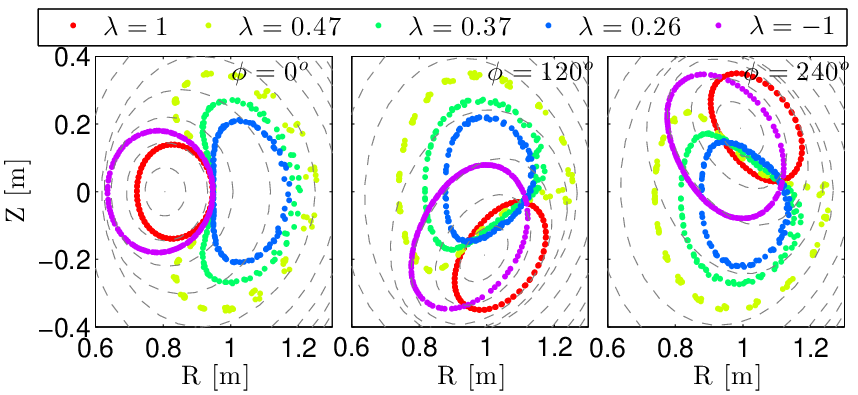

The magnetic axis naturally intersects some drift surfaces located in the core region such that orbits often pass through that singular point. This is a major difference with axisymmetric cases where difficulties with the magnetic axis only occur through collisional processes.
IV.0.3 Deeply-passing particles
The MAST Positive Ion Neutral Injector (PINI) emits neutrals at the energy of KeV. Larmor radii of trapped particles at these energies are a few centimetres large, but since injection is tangential, the kind of fast particles produced are almost exclusively deeply-passing particles, especially in the core region near the helical magnetic axis. It is instructive to focus on single particle orbits with initial pitch-variable close to unity (small magnetic moment). In particular, the guiding-centre equations of particles with a pitch-variable equal to unity (zero magnetic moment), yield constant. For such value of the pitch-variable, the drift surfaces associated to their motion are closest to flux-surfaces, as seen on figure 6. While all counter-passing particles travel around the original magnetic axis (see figure 7(b)), some co-passing particles circulate on drift surfaces that do not enclose the helical magnetic axis in the region of uncompressed flux-surfaces (see figure 7(a)). They move around a helical drift axis, positioned on the opposite side of the magnetic axis inside the kinked core. That behaviour is in part responsible for off-axis redistribution of NBI fast particles, evidenced by MAST neutron camera traces [17] and illustrated using a guiding-centre drift approach in slowing-down simulations [4].


In a full-orbit formulation, particles can develop small gyro-motion even if their pitch-variable is initially equal to unity (zero Larmor radius) depending on the bending of field-lines. The magnetic moment is not constant, but oscillates around an average value. In the case of helical cores, it is found that, even with strong field variations in the core region, full-orbit calculations of deeply-passing particles yield similar drift surfaces. Baños corrections to the drift equations are proportional to the magnetic moment, thus deviations are expected to be minimal for deeply-passing particles. Furthermore, the region of compressed flux-surface is geometrically very small such that few NBI particles are deposited in it. A low fraction of guiding-centres cross through this area, similarly to field-lines avoiding the region (see figure 5(a)). Previous results on NBI fast particle redistribution in the helical core of MAST is thus supported by this full-orbit analysis.
It is however reported that the investigation of fast particles with larger Larmor radii (ICRH or fusion alphas) in similar MAST magnetic configurations will probably require the use of higher-order GCDE or a full-orbit approach. The switching techniques described in section III in conjunction with the field variation criteria of section II would greatly help completing fast ion confinement simulations given moderate computational resources.
V Conclusion
In order to evaluate the limits of first order guiding-centre approximation, a method for estimating the total perpendicular variation of the magnetic field is proposed. It entails finding the largest eigenvalue of a matrix, composed of covariant derivatives of the magnetic field, projections and coordinate transformations. Although lengthy to expand on paper, this operation is easily performed on a computer and can be used within orbit simulations to quickly asses the validity of first order GCDE. It is also an instructive tool to probe the magnetic configuration for understanding its characteristics, i.e. regions of strong gradients, high curvature or large parallel currents.
A procedure to pass from guiding-centre to particle phase-space and vice-versa is described, that is employed when a particle enters or leaves a region of the magnetic configuration where the field variation is above a given threshold. Numerical resources are thus saved on particles with low energy for particles with larger Larmor radii. The switching technique is suitable for slowing-down simulations over long time-scales since the Monte-Carlo collision operators dilute the small error caused by the switching. With this algorithm, future simulations will yield more exact saturated fast ion populations, optimally using computational resources.
The field variation criterion is applied to a case of heavily distorted helical core equilibrium in MAST. It is reported that, for energetic particles of around KeV, the proposed field variation criterion reaches on the low-field side of the core and spikes in the narrow region where the flux-surfaces are compressed. The appearance of parallel currents explains the upsurge of field variation, as the pitch of field-lines varies extensively within a flux-surface and creates local shear.
Helical drift surfaces are obtained solving the particles’ full-orbits and tracing their guiding-centre trajectories. Confinement is guarantied by the existence of drift surfaces inside the core and by axisymmetry in the outer layers of the plasma. The kinked structure impacts on the deposition of NBI fast ions, as co-passing particles gather in the uncompressed flux-surface region. Full-orbit simulations confirm that the guiding-centre formalism was sufficient to model the NBI redistribution phenomena, mainly because NBI populations have small Larmor radii and close to zero magnetic moment. The investigation of more energetic and less tangential populations in MAST require however the use of higher-order GCDE or a full-orbit approach.
In future work, slowing-down simulations will benefit from the switching technique to yield saturated fast ion distributions that are exact even in strongly varying magnetic fields. The implementation of second order corrections to the GCDE will result in a lighter system of equations valid for intermediate field variations and an adjustment to the proposed criterion will be sought.
Acknowledgements
The authors are grateful to S. P. Hirshman for the use of the ANIMEC/VMEC code for the equilibrium simulations, to S. Brunner, L. Villard, D. Brunetti, J. Dominski and J. Faustin for insightful discussions. This work was supported in part by the Swiss National Science Foundation.
VI Appendix
VI.1 Charged particle orbits in a constant but sheared magnetic field
As an example of magnetic deformations that are completely ignored by the leading order terms of the guiding-centre approximation, it is instructive to solve the motion of charged particles in the constant, curvature-free but sheared magnetic field . Up to a gauge choice, the vector potential is . Hence the Lagrangian of such particle is written
The problem is integrable by virtue of the three constants of motion that can be deduced from the symmetries of the above Lagrangian:
Embracing the freedom of fixing the origin and orientation of the and axis, there is no loss in generality to consider the case where, at ,
i.e. , and . The non-linear coupled system of equations describing the motion of a charged particle respecting those initial conditions is then
| (11) | ||||
| (12) | ||||
| (13) |
where is the usual gyro-frequency. Equation (13) is similar to that of a pendulum, for which the solution is entirely expressed in terms of elliptic integrals. For , equations (11-13) properly reduce to those of a charged particle in a constant magnetic field pointing in the -direction, for which the solution is the well-known helical motion , and . In the special case where , the velocity along becomes constant, i.e. and the trajectory is circular in the plane, i.e. and with a radius of .
The motion in the -direction is bounded () only if
| (14) |
where is the maximum amplitude in the -direction. This condition demonstrates that if the Larmor radius is somewhat larger than the characteristic length of field-line shearing, particles do not necessarily perform a closed gyro-motion. If they do, the period of the closed motion is
where is the complete elliptic integral of first kind. The average velocity along the axis, which is the direction of the magnetic field at the guiding-centre position, is
where is the complete elliptic integral of second kind. By expanding at leading order in the shearing parameter , the correction to the average particle motion along the parallel direction is
| (15) |
The average parallel velocity is
Using (11-12) and after some algebra, the correction to the average parallel velocity is written
| (16) |
Therefore, at leading order, there is a difference between the average particle motion and the average parallel velocity
| (17) |
This paradoxical result is consistent with the so-called Baños drift [6, equation (37)], for which an interpretation is given in [19, appendix B] as well as in [7, p.718]. In this example of magnetic fields with no gradient nor curvature, the guiding-centre equations must be extended with second order terms in order to encompass the shearing of field-lines. In a Hamiltonian formalism, this can be performed starting with the second order guiding-centre Lagrangian derived in [3, equations (32-33)],
which yields Euler-Lagrange equation that coincides with (15)
| (18) |
The guiding-centre motion along the field-lines is thus different from the parallel velocity. The latter variable is interpreted in the guiding-centre phase-space as a pivot variable that includes the parallel curl of the magnetic field and the shearing of field-lines.
VI.2 Field variation estimation in various coordinates
VI.2.1 Toroidal coordinates with geometric toroidal angle
The field variation can be estimated with algebraic expressions of reasonable length in curvilinear coordinates where the toroidal angle is equal to the geometric angle. Derivatives of the magnetic field can be evaluated either in the covariant or the contravariant representation. For example, the matrix of interest is written
| (19) |
where are Cartesian coordinates, curvilinear coordinates. The perpendicular projection is the following contravariant tensor
the covariant derivative is
and the Christoffel symbol of first type is used
An other option is to lean on
| (20) |
where the covariant derivative is the mixed tensor
and the Christoffel symbol of second type is used
In theory, the two options (19-20) yield identical results but in practice, computing equation (20) is numerically more stable around the singular magnetic axis. In flux coordinates, divergent metric terms such as are naturally multiplied by terms going to zero like in the Christoffel symbol of second type . Such cancellation happens later in the matrix multiplication of (19) which makes it more prone to truncation errors.
VI.2.2 Cylindrical coordinates
In cylindrical coordinates , the metric is simpler
The Christoffel symbols of first type are mostly zero except for
Therefore the covariant derivative is written as
or alternatively
The perpendicular projection matrix is expressed as
VI.3 Small vector displacements in curvilinear coordinates
In Cartesian coordinates, is simply written , where are the Cartesian components of the Larmor radius vector. In curvilinear coordinates, the coordinates are formally written . This non-linear equation is simple to solve if the mapping from Cartesian to curvilinear coordinates is known. This mapping is not often provided and only the transformation from curvilinear to Cartesian is available. Then, one relies on root finding algorithms (slow) or linearisation (fast). For current applications, it is sufficient to expand at lowest order in gyro-radius, i.e.
| (21) |
where are the components of the Larmor radius in curvilinear coordinates. From prescription (9), those components are
where
Flux coordinates are however singular near the magnetic axis and this expansion can lead to wrong results when the norm of the basis vectors diverge. For this reason, it is preferable to linearise in a pseudo-Cartesian system. For example, if is a radial flux label, is a poloidal angle and is a toroidal angle, the pseudo-Cartesian coordinates are defined
where is the major radius and the minor. Then, the small displacement is written in the pseudo-Cartesian system as
where the jacobian matrix is easily obtained from (VI.3) and are again the components of the Larmor radius in curvilinear coordinates (21). After this operation, the coordinates are easily inverted back to the original curvilinear coordinates.
References
- [1] Northrop, T. G., Reviews of Geophysics 1 (1963) 283.
- [2] Boozer, A. H., Physics of Fluids 23 (1980) 904.
- [3] Littlejohn, R. G., Journal of Plasma Physics 29 (1983) 111.
- [4] Pfefferlé, D. et al., Nuclear Fusion 54 (2014) 064020.
- [5] D’Haeseleer, W., Flux coordinates and magnetic field structure: a guide to a fundamental tool of plasma structure, Springer series in computational physics, Springer-Verlag, 1991.
- [6] Baños, A., Journal of Plasma Physics 1 (1967) 305.
- [7] Cary, J. R. and Brizard, A. J., Rev. Mod. Phys. 81 (2009) 693.
- [8] White, R. B. and Chance, M. S., Physics of Fluids 27 (1984) 2455.
- [9] Belova, E. V., Gorelenkov, N. N., and Cheng, C. Z., Physics of Plasmas (1994-present) 10 (2003) 3240.
- [10] Boozer, A. H. and Kuo-Petravic, G., Physics of Fluids (1958-1988) 24 (1981) 851.
- [11] Albergante, M., Fasoli, A., Graves, J., Brunner, S., and Cooper, W., Nuclear Fusion 52 (2012) 094016.
- [12] Chapman, I. T. et al., Nuclear Fusion 50 (2010) 045007.
- [13] Cooper, W. A. et al., Plasma Physics and Controlled Fusion 53 (2011) 074008.
- [14] Hirshman, S. P. and Whitson, J. C., Physics of Fluids 26 (1983) 3553.
- [15] Cooper, W. A. et al., Computer Physics Communications 180 (2009) 1524.
- [16] Brunetti, D., Graves, J., Cooper, W., and Terranova, D., Nuclear Fusion 54 (2014) 064017.
- [17] Cecconello, M. et al., Nuclear Fusion 52 (2012) 094015.
- [18] Pfefferlé, D., Cooper, W., Graves, J., and Misev, C., Computer Physics Communications 185 (2014) 3127 .
- [19] Northrop, T. G. and Rome, J. A., Physics of Fluids (1958-1988) 21 (1978) 384.