Monte Carlo Search for Very Hard KSAT Realizations
for Use in Quantum Annealing
Abstract
Using powerful Multicanonical Ensemble Monte Carlo methods from statistical physics we explore the realization space of random K satisfiability (KSAT) in search for computational hard problems, most likely the ’hardest problems’. We search for realizations with unique satisfying assignments (USA) at ratio of clause to spin number that is minimal. USA realizations are found for -values that approach from above with increasing number of spins . We consider small spin numbers in . The ensemble mean exhibits very special properties. We find that the density of states of the first excited state with energy one is consistent with an exponential divergence in : . The rate constants for and of KSAT with USA realizations at are determined numerically to be in the interval at and at . These approach the unstructured search value with increasing . Our ensemble of hard problems is expected to provide a test bed for studies of quantum searches with Hamiltonians that have the form of general Ising models.
Keywords:
Spin Glass , Monte Carlo , Quantum Adiabatic Computation1 Introduction
Random satisfiability problems like three satisfiability (3SAT) and its generalization KSAT form a corner stone of complexity theory, a very active research branch in formal logic and computer science. In these theories one is concerned with logical forms defined on some bit space and one discusses the question whether or not there exists an assignment that turns the value of the logical form into “true”. The decision problem of KSAT and its accompanying function problem: the actual calculation of at given for belong to the class of NP complete theories [1], which for all practical purposes implies computational intractability. In these theories it is very common that worst case realization ensembles of forms exhibit an algorithm dependent complexity , that rises exponentially with the number of bits . The rate constants are smaller than the unstructured search value but at the same time can take values that are finite fractions of . This implies, that there exist problems which are not solvable even for small numbers of bits like , neither by analytic nor numeric methods, even usung brute computational force.
It is the privilege of statistical physics to turn the abstract notion of satisfiability into studies of Hamiltonian systems upon mapping the bit degrees of freedom via for to Ising degrees of freedom , and upon introducing a suitable Hamiltonian whose ground-states at energy map one by one to the satisfying assignments of . One may either consider classical statistical physics where the theory is supplied by artificial thermal fluctuations at inverse temperature within the framework of the canonical partition function or alternatively, consider the quantum statistical theory of Pauli spins and with the quantum partition function
| (1.1) |
where quantum fluctuations at low are tuned via an external parameter . For both cases the mathematical intractability is encoded into physical theories and it is an exciting research topic to study its consequences i.e., phase transitions and correlations from various points of view. For the classical theory it was shown, that computational intractability is related to a phase transition - the SAT transition - along the principal parameter direction of random KSAT theories [2], the ratio hereby denoting the ratio of clause to spin numbers. In a later effort complexity related observables were determined analytically within the framework of replica symmetry breaking theory for random 3SAT [3], and also numerically in large scale simulations [4]. In particular the critical point of the 3SAT transition was determined to be analytically. For the quantum theory, and within quantum information theory it was conjectured that adiabatic quantum computations (AQC) based on the properties of could possibly obtain ground states of in polynomial physical time [5, 6]. For hard 3SAT realizations it turned out however, that early findings on polynomial ground state search times had to be corrected to exponentially large ones [7] for the simplest case of AQC making use of a transverse magnetic field and a linear -parameter schedule. A similar finding was made recently for a another satisfiability theory: Exact Cover [8].
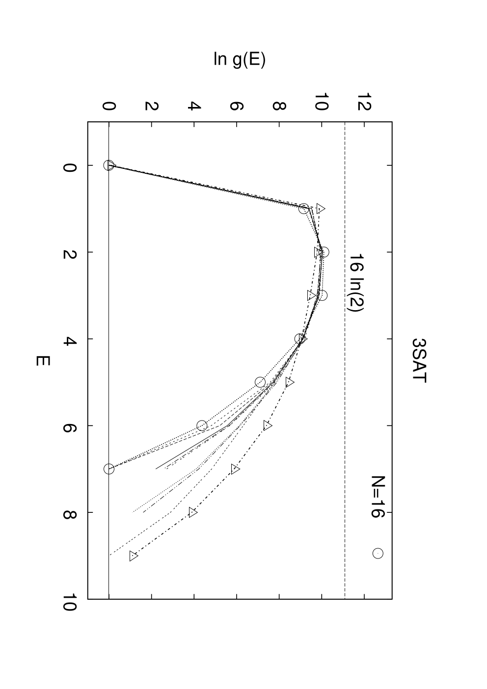
Within the current work we execute a very use-full exercise prior to the actual studies of complexity related observables in physical theories. We restrict the admissible set of all KSAT Hamiltonians, namely random KSAT realizations with ensemble mean , to a much smaller ’hard’ set of Hamiltonian’s with corresponding ensemble mean. The index denotes the ensemble members which for reasons of computer time limitations have finite number throughout the paper. As far as ground-state searches are concerned our problem set is targeted at hard problems - most likely the ’hardest problems’ - which otherwise and within are exponentially rare. Our problems are constructed under specific constraints:
- 1.
The ground-state to any is unique, which if denotes the density of states function (DOS) implies . Such problem realizations possess unique satisfying assignment’s (USA).
- 2.
For a given number of spins and for realizations with the number of clauses is minimal. The parameter is then minimal too . E.g. : we find that USA realizations in 3SAT for follow .
- 3.
The set of problem realizations is drawn with unique probability from the set of realizations.
Similar realizations have lately been considered for 3SAT in Ref. [9] with a weaker constraint on the value , which had the value . The minimal KSAT values within this work turn out to approach from above independent of with increasing . In short: we are constructing USA realizations in KSAT at asymptotically.
At the heart of our numerical calculations is a Markov Chain Monte Carlo study of the partition function
| (1.2) |
which partitions the realization space of random KSAT within respect to , the ground-state multiplicity. Once the Markov Chain Monte Carlo visits the sector (USA) corresponding problems are collected on the disk of a computer. Similar flat histogram sampling methods, like Wang-Landau [10] and Multicanonical [11] simulations have recently been used in complexity theory in an attempt to sample the density of states function in 3SAT for spin numbers that prohibit exact enumeration [12]. The final part of the paper classifies measures of complexity within typical problem realizations in .
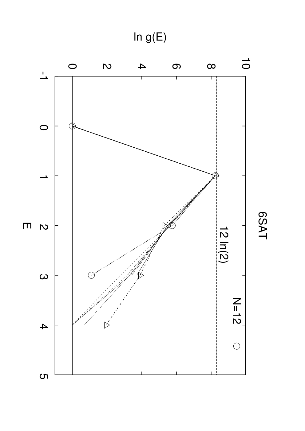
Today’s understanding on the origin on the complexity of the physical search in frustrated and disordered systems pictures a free energy landscape in which as a function of the value , a finite number of solution clusters is accompanied by an exponentially large number of almost solution clusters at energy near but above the ground-state. All clusters are separated by finite free energy barriers. The situation resembles the search for a needle - or several needles - in a haystack. A simplified mechanism operates within our hard problem ensemble . We find, that the phase space volume at is exponentially large in the number of degrees of freedom , see the examples of displayed in Fig.(1). Thus first: for all of the considered KSAT theories with up to we encounter the generic situation: a single needle is searched in a haystack of exponential large size 11 1 The theories at are NP-complete while at there exist mathematical polynomial time algorithms that find the ground-state even though is exponentially large.. Second: we find numeric evidence that actual values of are extremal i.e., maximal under the condition of minimal , which in turn justifies the notion of most likely the ’hardest problems’.
2 Theory, Hard Problems and Monte Carlo Simulation
2.1 Theory and Observables
In KSAT one considers logical forms - a function - whose truth value can either be true or false and which are defined on a space of Boolean degrees of freedom - bits - with . In the satisfiability problem one asks for the existences of assignment’s i.e., bits that would evaluate the function at the value true. Solving the function problem implies the explicit calculation of a single satisfying assignment or, of all different satisfying assignments if there are several of those. The logical form is the conjunctive normal form of clauses : , which only evaluates true if all clauses with evaluate true simultaneously. Any of the clauses is the disjunction of integer literals with and :
| (2.1) |
A clause is true, if at least one of its literals evaluates true. For example, in 3SAT there are configurations of literals on the clause which evaluate true and just one with truth value false. In addition, a literal is either a bit or its negation and, the actual identification of a literal with a specific bit - or its negation - is controlled by a map , that associates clauses and clause-positions to the index set of bits. The map and the possibility of negations at the literal positions are free parameters of the theory. In an Hamiltonian theory they can be used to introduce ensembles with mean over random disorder as well as random frustration, a possibility that is heavily exploited in this work. It is implicitly understood, that tautologies i.e., contradicting pairs within clauses like as well as redundancies i.e., duplicate literals like or are not admitted to the theory.

The physical degrees of freedom are classical Ising spins with and without loss of generality, true on each bit is identified with spin up . Let us introduce functions in an attempt to write the Hamiltonian as a sum of terms: , where each term corresponds to a clause and, where the ground-states of at energy can be identified one by one with the satisfying assignments of . For this purpose we note that spins of the clause add up to the sum , which takes different values . Consequently the polynomial
| (2.2) |
has the value for all spin configurations except one, if only all spins are down: with . For the latter case , which implies an energy-gap of value unity. For the function is a linear combination of the spins n-point functions , , … , with a maximum of value . For purposes of illustration we present the 2SAT and 3SAT cases. For 2SAT we obtain the anti-ferromagnet at finite field
| (2.3) |
while in 3SAT
| (2.4) |
The necessary frustrations are encoded in a matrix array which for each clause and position with follows the pattern of negations within , a negation induces an while otherwise . We mention that in random KSAT, which we denote by the ensemble mean , values of are drawn with equal probability . The final form of the KSAT Ising Hamiltonian is
| (2.5) |
and is the basis of our studies. Its principal parameters for are the ratio of clause numbers over namely , and the particular assignments of spins to clauses via the map , as well as the settings within the frustration matrix . We denote a specific setting of the latter map and matrix a realization and study ensemble mean expectation values of observables at fixed throughout the paper.

Once the Hamiltonian is given we formally define the canonical partition function which at temperature allows the definition of physical observables as there are the internal energy , or the specific heat . The canonical partition function has the spectral representation
| (2.6) |
where denotes the density of states (DOS):
| (2.7) |
For KSAT theories is integer valued, has finite support on the integer values of the compact interval and an integral . A satisfiable Boolean form induces , while corresponds to an that only has one unique satisfying assignment (USA). Boolean forms, that cannot be satisfied have . The quantity also is denoted the microcanonic phase space volume of the energy one energy surface.

Our knowledge of the statistical properties of K satisfiablity stems from extensive analytical [3] and numerical studies [2] of random KSAT, which have demonstrated the existence of a transition, possibly a phase transition at values . The SAT to UNSAT transition separates at low a phase where formulas are satisfied in the mean, from a phase at large where formulas can not be satisfied. Numerical data for the probability of un-satisfiable formulas within the mean of random KSAT are displayed in Fig.(2) and illustrate the statement. The data are of similar quality as the data obtained by Selman and Kickpatrick in 1996 [2]. The consensus is that probable realizations within random KSAT are ’hardest’, i.e. computational most intractable, at and in the vicinity of the transition point . However, this does not exclude the existence of still ’harder’ i.e., worst case realizations which at arbitrary are hidden in the tails of probability distribution functions for complexity related observables with small, possibly very small probabilities.
2.2 Search for Hard Problems
The starting point of our search for ’hard’ realizations are observations that concern realizations with USA. If one considers USA realizations in 3SAT for the smallest spin number and clause number one inevitably arrives at the realization
| (2.8) |
which encodes the unique ground state . This particular example is one of eight that all encode USA’s for , and is turned in a readable form upon permuting clause and literal indices. It has interesting specific properties:
- 1.
FOR is the minimal form with a USA. For and there are no USA realizations in 3SAT.
- 2.
The density of states only has two values and . All spin flips acting on the ground-state lift the energy surface by just one unit to . The states with have dis-proportional large multiplicity and therefore is hidden. This suggests that still ’minimal’ but larger forms at values could inherit a similar property. These must exist at as one can introduce additional spins and clauses one by one. For example, if we introduce a fourth spin and extend by one clause to an form with comparable property, then
(2.9) The latter form encodes the unique ground state and has the density of states and respectively. Again configurations have large multiplicity.
- 3.
Within of eq.(2.8) there are exactly clauses - those with two negations - which in the unique solution are solved by just one true literal. There are in addition clauses which are solved by two literals and clauses which are solved by three literals. Also, there exists a polynomial transformation of 3SAT to maximal independent set (MIS) [13]. It is easy to show, that a unique ground-state of the 3SAT problem transforms into a degenerate ground-state in the corresponding MIS problem. The ground-state multiplicity MIS, , has the value
(2.10) on . We note that of turns out to be while and remain having values and , and thus also is constant at . It is suggested that ’minimal’ but larger () forms can have indices that are of magnitude , which in turn limits the volume to finite values. Finite values imply vanishing ground state entropy density under the polynomial transformation from 3SAT to MIS.

The existence of examples with interesting properties guides our expectations. The question is raised whether USA and 3SAT realizations at the ratio of clause to spin numbers
| (2.11) |
exist for arbitrary and what their properties are ? In absence of useful mathematical methods we use Monte Carlo simulations in order to actually construct members of the ensemble at , and in a later measurement step we determine their properties. In particular we calculate , the multiplicity of the energy one surface. It is then necessary to employ biased Monte Carlo sampling techniques, as in the vicinity of USA realizations within random 3SAT have exponentially small probability. Finally it is easy to generalize our arguments to arbitrary . For KSAT with we expect USA realizations with minimum clause number at
| (2.12) |
under the condition that .
2.3 Monte Carlo Search and Checks
The Monte Carlo simulation performs a stochastic estimate of the biased partition function
| (2.13) |
which for is evaluated on the phase space of all possible random KSAT realizations for a given KSAT Hamiltonian eq.(2.5). The bias, as expressed by the Boltzmann factor , is introduced along the lines of Multicanonical Ensemble simulations [11] and serves the purpose to lift the probabilities of rare configurations in the Markov chain. The Monte Carlo is expected to perform a random walk in and whenever the sector is visited an ensemble member of is stored on the disk of a computer. Our Monte Carlo is quite un-conventional and essential remarks are in order:
- 1.
The Markov chain of configurations consists of realizations as specified by their maps and frustration matrix . Each problem realization is attached to a Hamiltonian theory with density of states that can be evaluated at , . The calculation of for a given configuration unfortunately takes computational steps. Our Monte Carlo simulation therefore is limited to small numbers of spins. We studied KSAT theories for and . We were able to generate ensembles of statistical independent members each for maximum spin numbers and respectively. Minimum spin numbers always are ..
- 2.
Configurations are updated with Metropolis updates [14]. The initial problem realization at is subject to a trial-update which targets . The Markov chain accept probability for the move is
(2.14) and as usual, if the update is rejected the initial configuration stays within the Markov Chain.
- 3.
Trial updates are generated randomly on the space of random KSAT realizations. One chooses a random clause and clause position and at trial values and , which are uniformly distributed on the measure of the theory. The absence of redundancies and tautologies constrains the admissible move set. The typical number of Monte Carlo moves for the simulation of is . For the larger values it was necessary to repeat the simulations with different random number sequences possibly 10, up to several 10 times. The numerical data, as presented in the paper, consumed one month of computer time on a processor workstation cluster.
- 4.
The biased partition function of eq.(2.13) serves as a tool to facilitate Monte Carlo sampling of different sectors in random KSAT and in particular the sector (USA) is sampled efficiently. There is however an additional benefit. After finishing the biased Monte Carlo simulation a final reweighing step restores the un-biased partition function
| (2.15) |
which on the space of random KSAT realizations simply counts the probability of multiplicities . Given we can determine expectation values of known observables within random KSAT, which provide consistency checks on the correctness of the Monte Carlo simulation. A list and a comparison to numerical data follows:
- 1.
In random KSAT there is always a finite probability of problem realizations with non-vanishing multiplicity. In fact one can calculate the mean multiplicity
(2.16) on combinatorial grounds at arbitrary exactly [12], which simply yields
(2.17) In Fig.(3) we compare selected measurement data for with the exact result for various values of , and . The Monte Carlo data agree with the combinatorial result very well.
- 2.
One may wonder whether a theory with an entirely regular will contain a non-regular structure at the SAT to UNSAT transition . However, the constraint expectation value of the quantity , under omission of the sector does in fact show non-trivial behavior. Within the SAT phase it equals the ground-state entropy density , for which long time ago [15] and for the theories 2SAT and 3SAT an series-expansion was calculated within replica symmetry breaking theory up to order . In Fig.(4) we compare our numerical data in 2SAT and 3SAT with the series expansions results. The figure contains two curves, which for 2SAT for and for 3SAT for are indistinguishable from the numerical data points. Finally we note for random KSAT, that the probability of an un-satisfiable formula has the simple representation
(2.18) The data are displayed in Fig.(2).
The main reason for the use of quite elaborate Monte Carlo techniques is the rareness of USA realizations for , in particular for the conjectured exact point , as given in eq.(2.12). For all our theories with and and for typical like we search the -parameter space also at -values below for USA realizations. Neither Multicanonical Ensemble simulations for several weight functions , nor Wang Landau simulations or, alternatively simulated annealing runs in - ever produced a USA realization for below . However, at eq.(2.12) USA realizations are found. The relative probability for the occurrence of unique satisfying assignment’s within random KSAT is
| (2.19) |
We display in Fig.(5) data in 3SAT for spins. appears to be a slowly varying function above , with a maximum around and with a rapid decrease towards minimal and very small values at and, problems with larger appear to be increasingly improbable. The asymptotic decay of is consistent with an exponential decay with in 3SAT and is depicted in the inset of Fig.(5). In addition at fixed spin number values of turn out to be even smaller if larger values are considered. We quote and for the twelve spin theory with and in 4SAT. Finally we present for purposes of illustration a specific 3SAT realization for spins and clauses:
| (2.20) |
For it encodes the unique ground state - zero corresponding to spin down and one corresponding to spin up - and is characterized by the phase space volumes , and . USA realizations for the given parameter values have probability to occur by chance within random 3SAT. The full density of states of eq.(2.20) is depicted in Fig.(1), see the triangles in the figure. Finally the stochastic nature of the Monte Carlo search result is apparent if one compares the random structure of eq.(2.20) with the regular structure in eq.(2.8).
3 Properties of Hard KSAT Realizations

2 0.34762(112) 0.65 3 0.56918(096) 1.87 4 0.63620(015) 0.66 5 0.66574(025) 2.55 6 0.67934(014) 0.30
For each of the generated problem realizations within the ensemble and as defined by the partition function of eq.(2.15) for , we calculate the density of states eq.(2.7). We determine its mean on the surface
| (3.1) |
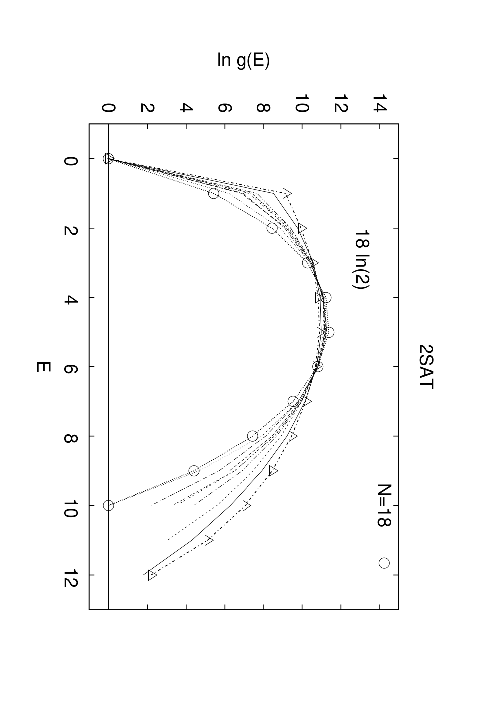
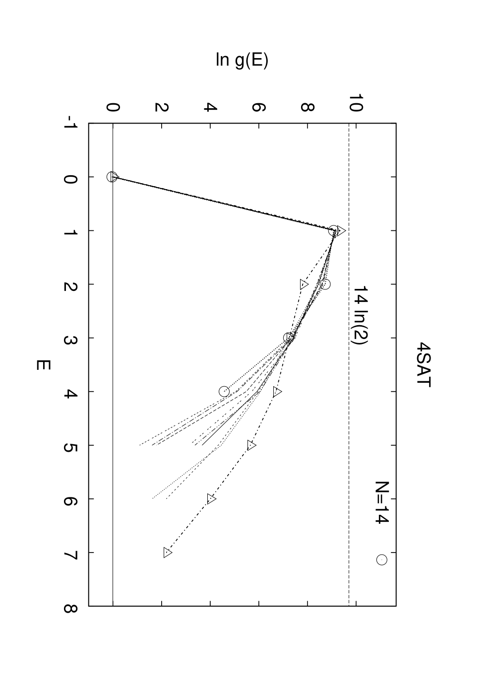
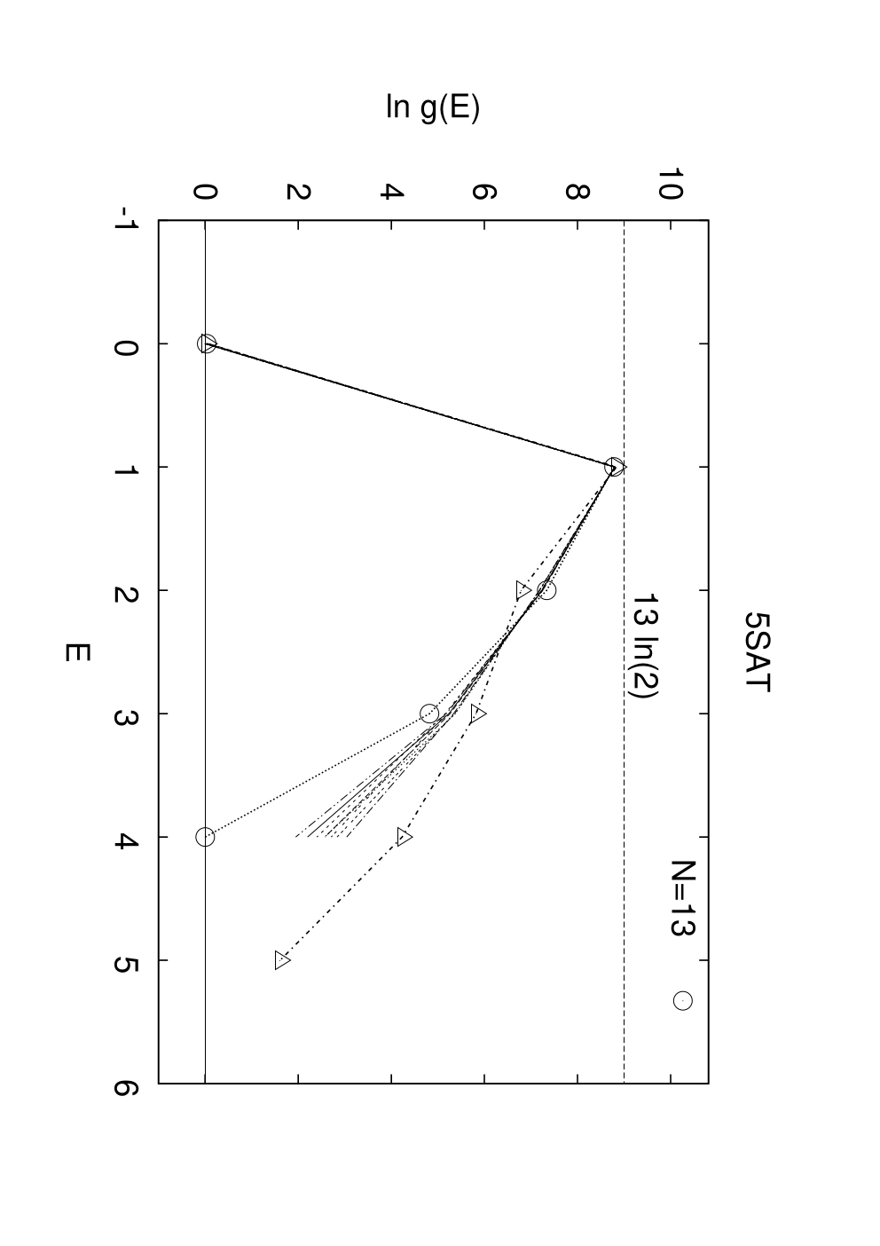
Selected data for the density of states with are displayed in Figures Fig.(6) and Fig.(7) for the KSAT theories. They complement the 3SAT data displayed in Fig.(1). In each case the multiplicity of configurations exhibits a step that is of magnitude for the given number of spins . Our final numerical data for the mean multiplicity of configurations , in the theories 2SAT, 3SAT and 6SAT are displayed in Fig.(8). The numerical data are consistent with an exponential growth
| (3.2) |
for large values of with finite growth rate constants . Subsequently, we performed fits to the data in order to determine the shape of the singularity eq.(3.2) and to measure values of the rate constants in KSAT theories with . Restricting the fit interval to the cases with we obtain acceptable -values for the fit. The final rate constants and -values of the fits are contained in Table 1. The -dependence of the rate constants is also depicted in the inset of Fig.(8). Starting from a moderate value for the rate constant in 2SAT, , we obtain in 3SAT and, beyond the rate constants rapidly approach the unstructured search value . For 6SAT the rate constant is .

A classical statistical model with a density of states , that squeezes an exponential large number of configurations into the first energy level above the ground-state, see the right panel of Fig.(7) is certainly a very special theory. Let us recall the ferromagnetic Ising model, which in any dimension has a ground-state degeneracy as well as a multiplicity at the first energy level. Polynomial singularities in are the consequence of theories with local interactions. However, the class of problems considered here does not possess this property.

The spin configurations at energy will have a phase space distribution and it is interesting to know, whether that distribution is biassed towards the ground state configuration. For this purpose we calculate the overlap to the ground state
| (3.3) |
where denotes ground state spins. For purposes of illustration we display in in Fig.(10) the number histogram for a single problem in 2SAT. We obtain a bell-shaped overlap distribution which actually is slightly biassed away form the ground state to the negative half space. We note that the histogram carries entries at and thus the ground state is accessible via single spin flips from the surface. We also have analyzed the connectivity of configurations. Using ballistic shooting we find that any two configurations are connected by sequences of single spin flips without leaving . This is different from spin glasses where in general there are several connectivity components and corresponding free energy barriers. Any single spin flip dynamics e.g. Metropolis updates can easily explore the surface.

We also consider the canonical ensemble eq.(2.6). We calculate the internal energy with , as well as the specific heat , as a function of the inverse temperature . For 3SAT we display and for and spins in Fig.(11). A theory with a finite energy gap is expected to possess a freezing phase transition at low, possible very low temperatures below which and for values the internal energy approaches its asymptotic ground-state value . The numerical data in fact confirm the presence of freezing, with a position as given by the position of a pronounced peak in the specific heat, see the inset of Fig.(11). Figure (9) displays data in 3SAT, which as a function of exhibit a blatant linear dependence, see the straight lines in Fig.(11). We remark that at the freezing point configurations with coexist with a single configuration at the ground-state energy.

A popular algorithm within the canonical ensemble for the solution of optimization problems is simulated annealing (SA) [16]. Simulated annealing runs will have to use temperature annealing schedules with temperatures low enough to reach the freezing point at e.g. for 16 spins in 3SAT and, then will have to explore number of possibilities to finally arrive at the ground-state. The process will consume an exponentially large amount of time, if is exponentially large. We do not expect, that other algorithmic improvements like kinetic Monte Carlo methods [17] can avoid the exponential singularity.
We have implemented simulated annealing for the problem set in 3SAT. We use the canonical partition function eq.(2.6) and choose a random initialized spin-configuration. We then perform local Metropolis spin updates in a multi-spin coded computer program [18, 19]. We employ compute time farming on a parallel computer with a parallel random number generator of Marsaglia [20]. Each annealing trajectory is started at the very high temperature
| (3.4) |
and terminates after Sweeps i.e., Monte Carlo steps where is the spin number, at the exact temperature
| (3.5) |
We use a polynomial temperature schedule
| (3.6) |
where is the sweep number and constants are determined to meet the boundary conditions on the temperature. For each problem we repeat the annealing trajectories times with different random numbers and determine the mean success probability with of successful ground-state searches after the sweep has been finished. Our measure of SA search run-time is
| (3.7) |
at target success rate one-half : . The procedure is repeated for a possible realizations and at all values of . The correlation of run-times with the density of states is linear for 3SAT, as can be inspected in Fig.(12) for a selected set of problems at various . These run times are quite short. If e.g. at the energy surface has degenerate spin configurations a typical number of Monte Carlo Steps is sufficient to solve the problem at a success rate of one half. However if the target success rate is demanded to be very close to unity larger times are needed. Our findings imply that the classical compute time for solving problems with simulated annealing goes like with values as given in Table 1. It is this kind of singularity a quantum search has to compete with.
4 Conclusion

Within the scope of the present work, we have generated prototype problem realizations within KSAT theories, which under the constraint of a unique satisfying assignment (USA) at minimal clause number develop extremal statistical properties. The phase space volume at the minimal energy gap is exponentially large and likewise for a given KSAT theory maximal. The idea was formulated in by Znidaric [9] but in absence of efficient Monte Carlo methods it was not worked out at minimal clause number and at large values of the rate constants . The class of problems as presented here exemplifies our current understanding of physical search complexity in random systems in a straight and simple way: A single ground state is hidden in an exponentially large phase space volume at the first energy gap. For the theories with large almost all spin configurations are collapsed to the surface, except the one ground state configuration at . In this situation there exists no distance measure or cluster property which within the surface would allow the detection of a direction, as to where the ground state could be searched for. Representatives of the ensemble can be obtained at request from the author.
The given problems at and in this work are constructed on problem Hamiltonians that contain higher order interactions of spins like . From a physics point of view it would possibly be nicer to eliminate such unphysical couplings and stay with only 2-point spin couplings, as well as magnetic fields. We mention that all the Hamiltonians at can be transformed via polynomial transformations to Maximal Independent Set (MIS),see [13], which in fact can be represented by 2-point and magnetic field spin couplings only. It is plausible to assume that these after polynomial transformation retain their “hardness”.
The design of problem realizations with specific properties facilitates the subsequent study of proper defined search efficiency’s in processes, that can possibly be implemented on a physical device e.g., a quantum computer. For purposes of illustration we mention here quantum annealing within the quantum partition function of eq.(1.1). Search times for ground-state calculations via quantum annealing are expected to be bounded by below through a gap-correlation length , which is determined from spin-spin correlations along the imaginary Trotter Suzuki time of at the quantum critical point. For 3SAT we present in Fig.(13) preliminary numerical results for in the median average of the hard problem ensemble. The data, as indicated by the straight line in the figure, show in fact also an exponential singularity of a similar type as in eq.(3.2), that now is governed by a quantum rate constant , a value that is close to of Table 1. The caveat however is, that in presence of a Landau Zener avoided level crossings quantum run-times for linear quantum annealing schedules show a quadratic singular behavior [21], which leaves the quantum search efficiency far behind the classical search. Similar exponential singularities at smaller values of were already observed for quantum 3SAT on a set of ’weaker’ problems [7]. A detailed study of quantum search complexities on the set of hard problems in 2SAT has just been completed [22] and complements the less physical findings of this work.
Finally we mention that the spin numbers in this work are embarrassing small, as the Monte Carlo search on the problem set consumes exponentially large resources. We can safely say that with current methods it is not possible to generate a corresponding ensemble of problems even for spin numbers as small as . It is however not excluded, that single problem representatives can be found by clever heuristic construction. We emphasize that we do not want to give up the ensemble property because otherwise we would be studying arbitrary mathematical problems. This will be relevant for search complexity distributions which are expected to exhibit ensemble properties.
Acknowledgement: Calculations were performed under the VSR grant JJSC02 and an Institute account SLQIP00 at Jülich Supercomputing Center on various computers.
References
- [1] S. A. Cook, Proc. Third Annual ACM Symposium on the Theory of Computing, (ACM, New York, 1971) 151.
- [2] B. Selman and S. Kirkpatrick, Artificial Intelligence 81, Issues 1-2, (1996) 273.
- [3] M. Mezard, G. Parisi and R. Zecchina, Science 297,(2002) 812.
- [4] A. Mann and A. K. Hartmann, Phys. Rev. E 80, (2009) 066108.
- [5] T. Kadowaki and H. Nishimori, Phys. Rev. E 58, (1998) 5355.
- [6] E. Farhi, J. Goldstone, S. Gutmann, and M. Sipser, arXiv:quant-ph/0001106, (2001); E. Farhi, J. Goldstone, S. Gutmann, J. Lapan, A. Lundgren, and D. Preda, Science 292, (2001) 472.
- [7] T. Neuhaus, M. Peschina, K. Michielsen and H. De Raedt, Phys. Rev. A 83, (2011) 012309.
- [8] A. P. Young, S. Knysh, and V. N. Smelyanskiy, Phys. Rev. Lett. 101, (2008) 170503 and Phys. Rev. Lett. 104, (2010) 020502.
- [9] M. Z̆nidaric̆, Phys. Rev. A 71, (2005) 062305 .
- [10] F. Wang and D. P. Landau, Phys. Rev. Lett. 86, (2001) 2050.
- [11] B. A. Berg and T. Neuhaus, Phys. Rev. Lett. 68, (1992) 9.
- [12] S. Ermon, C. Gomes and B. Selman in “A Flat Histogram Method for Computing the Density of States of Combinatorial Problems”, IJCAI 2011, Proceedings of the 22nd International Joint Conference on Artificial Intelligence, Barcelona, Catalonia, Spain (2011).
- [13] V. Choi in "Adiabatic Quantum Algorithms for the NP-Complete Maximum-Weight Independent Set, Exact Cover and 3SAT Problems", arXiv:1004.2226v1 [quant-ph] (2010).
- [14] N. Metropolis, A. Rosenbluth, M. Rosenbluth, A. Teller and E. Teller, Journal of Chemical Physics 21 (1953) 1087; W. K. Hastings, Biometrika. 57 (1970) 97.
- [15] R. Monasson and R. Zecchina, Phys. Rev. E 56 (1997) 1357.
- [16] S. Kirkpatrick, C. D. Gelatt and M. P. Vecchi, Science 220 (1983) 4598.
- [17] A. B. Bortz, M. H. Kalos and J. L. Lebowitz, Journal of Computational Physics 17 (1975) 10.
- [18] S. Wansleben, J. G. Zabolitzky and C. Kalle, J. of Statist. Phys. 37, Issue 3-4 (1984) 271.
- [19] G. Bhanot, D. Duke and R. Salvador, J. Stat. Phys. 44, Issue 5-6 1986) 985.
- [20] G. Marsaglia, J. Stat. Software 8, 14, (2003) 1.
- [21] C. Zener, Proceedings of the Royal Society of London A 137 (1932) 696.
- [22] T. Neuhaus, “Quantum Searches in a Hard 2SAT Ensemble”, preprint, November 2014.