Thermodynamics of the Topological Kondo Model
Abstract
Using the thermodynamic Bethe ansatz, we investigate the topological Kondo model, which describes a set of one-dimensional external wires, pertinently coupled to a central region hosting a set of Majorana bound states. After a short review of the Bethe ansatz solution, we study the system at finite temperature and derive its free energy for arbitrary (even and odd) number of external wires. We then analyse the ground state energy as a function of the number of external wires and of their couplings to the Majorana bound states. Then, we compute, both for small and large temperatures, the entropy of the Majorana degrees of freedom localized within the central region and connected to the external wires. Our exact computation of the impurity entropy provides evidence of the importance of fermion parity symmetry in the realization of the topological Kondo model. Finally, we also obtain the low-temperature behaviour of the specific heat of the Majorana bound states, which provides a signature of the non-Fermi-liquid nature of the strongly coupled fixed point.
Keywords:
topological Kondo , thermodynamic Bethe ansatz , Majorana , non-Fermi-liquid , star junctionPACS
05.30.Fk , 71.10.Pm , 73.22.-f , 73.63.Rt1 Introduction
The possibility of faithfully simulating quantum low dimensional systems gives today the unique opportunity of testing against experiments predictions made by powerful methods – such as bosonization [1] (see also Schulz et al. in [2]), conformal field theory [3], integrable models and Bethe ansatz [4] – developed in theoretical investigations of strongly correlated condensed matter and spin systems. As a result, one may now confidently apply the above methods to newly engineered quantum systems relevant for the fabrication of quantum devices as well as for the realization, in a easily controllable setting, of new phases of matter such as the non-Fermi liquid phases realized in Dirac materials [5] and in overscreened multi-channel Kondo models [6]. Within the new models made accessible to theoretical investigations, great opportunities are offered by the analysis of pertinent junctions of one dimensional systems such as ladders and star junctions [7, 8, 9, 10, 11, 12].
Networks of one dimensional models attracted much attention over the past few years. In pioneering works [13, 14] a star junction of three quantum wires enclosing a magnetic flux was studied: modelling the wires as Tomonaga-Luttinger liquids (TLL), the authors of Ref. [13, 14] were able to show the existence of an attractive finite coupling fixed point, characteristic of the geometry of the circuit. Later, a repulsive finite coupling fixed point was found in a T-junction of one dimensional Bose liquids [15]. Crossed TLL were also the subject of many investigations both analytical [16] and numerical [17]: these analyses pointed out that, in crossed TLLs, the junction induces behaviours similar to those arising from quantum Kondo impurities in condensed matter physics [18]. For what concerns the analysis of junctions of spin chains, in ref. [19] it was argued that novel critical behaviours emerge when crossing at a point two spin Heisenberg models since, as a result of the crossing, some operators turn from irrelevant to marginal, leading to correlation functions exhibiting power law decays with non-universal exponents. Star junctions of Josephson junction arrays were investigated in [20] with the result that a finite coupling fixed point was also emerging in these superconducting systems. With Majorana fermions [21] star junctions of quantum wires become very attractive since these geometries facilitate their braiding [22] allowing, at least in principle, for the engineering of quantum circuits relevant for the implementation of quantum protocols [23, 24].
The very close relation between the phase diagram emerging from the investigation of networks of quantum one-dimensional systems (quantum spin chains and quantum wires, essentially) and the one typical of multichannel Kondo models was established only very recently. In the two papers [25, 26] it was shown that a star junction of three critical Ising models and a star junction of three XX models may be made equivalent to the two channel and the four channel over-screened Kondo model, respectively. To achieve their exact mapping, these authors used a generalization of the Jordan-Wigner transformation needed to satisfy the anticommutation relations between fermions located on different legs of the junction. For this purpose, one modifies the usual Jordan-Wigner transformation by the addition of an auxiliary space made - for a star junction of three spin chains - by three Klein factors, i.e. three real anti-commuting fields, lying at the inner boundary of each chain. As a result, in these realizations of the multichannel Kondo model, the central spin, with which the Jordan-Wigner fermions interact, is realized as a non-local combination of three Klein factors. The Kondo effect occurring when bulk fermions scatter on a composite “spin” non-locally encoded by any number of Klein factors located at different space points provides a realization of the topological Kondo effect. Since one expects that an extended spin is less sensitive to noise and decoherence, it is generally believed that this realization of Kondo models could “naturally“ be much more robust than the one realized by other means (for example with quantum dots [27]).
In an effort to look for new experimental realization of a two-channel Kondo Model the authors of [28, 29] showed that, in pertinent circuit regimes, networks of quantum wires supporting edge Majorana modes [30] provide a first experimentally attainable realization of the so-called Topological Kondo effect. Subsequently, the spin dynamics [31], as well as the exact solution for finite number of electrons [32], was investigated. In realistic cases the topological Kondo effect may be realized in networks of quantum wires supporting edge Majorana modes. For instance, it takes place when a mesoscopic superconducting island, capacitively coupled with the ground, hosts a set of Majorana bound states, which may be the Majorana edge modes (MEMs) of a set of spin-orbit coupled nanowires (green in figure 1 in colour version) laying on this superconductor. Note that, in this realization, the MEMs always appear in pairs, localized at the opposite ends of the nanowire. As a result, the central region of a circuit realizing the topological Kondo effect contains always an even number of MEMs. Nevertheless, it is always possible to couple only an odd number of MEMs to external wires, thus leaving an odd number of Majorana modes decoupled from the rest of the system.

Coulomb interactions among the electrons within the external leads are not essential for the topological Kondo effect and will not be accounted for in the following. However, for the host superconducting region, they play an essential role, since they determine its charging energy [28, 31]. We focus on the temperature regime , which implies that, for all real processes, the number of electrons on the island is conserved. We emphasize that, at least at low temperature, the MEMs must be the only degrees of freedom in the central region which are involved in the dynamics. Under these conditions, the effective low-energy Hamiltonian describing the TKM is [28, 29, 33, 34]
| (1) | |||||
and, manifestly, preserves fermion parity. Here are the (complex) Fermi fields describing electrons in the wires and satisfying canonical anticommutation relations
| (2) |
while the are Majorana fields constrained in a box connected with the wires and satisfying the Poisson algebra
| (3) |
The symmetric matrix is the analogue of the coupling with the magnetic impurity in the usual Kondo problem. The couplings represent a direct interaction between only a pair of Majorana fermions and can be made exponentially small by considering the MEMs sufficiently separated in space [35]. This model coincides with the one studied in [32]. A related, yet different model, with real spinless fermions in the bulk, has been analysed in [36].
If of the MEMs are coupled to the external wires, this set of MEMs may be regarded as a "Majorana spin": in contrast to a conventional spin the ”Majorana spin” is non-locally encoded in the spatially separated MEMs and governed by the orthogonal symmetry group . It has been found [28, 29, 33, 34] that the topological Kondo model (TKM) provides a natural realization of the quantum critical point described by a Wess-Zumino-Witten-Novikov boundary conformal field theory [37, 38, 39, 3] and support non-Fermi-liquid ground states.
In this paper, using the thermodynamic Bethe ansatz (TBA), we investigate the thermodynamics of the TKM with an arbitrary number of wires . For this purpose, we study a system with a thermodynamically large number of electrons in contact with an heat bath at temperature and at fixed density and perform the thermodynamic limit as in (12). Our analysis allows to derive the free energy of the TKM for arbitrary number of external wires, to compute the ground state energy as a function of the number of wires and of their couplings to the Majorana modes, as well as the low temperature behaviour of the specific heat of the central region.
An outline of the structure of the paper and of our results is as follows: In section 2 we review the exact solution of the TKM, as provided in [32].
In section 3 we derive the exact free energy of the TKM made by wires coupled with MEMs in the central region. Here, we write the TBA equations for both even and odd . In section 3.3 we obtain, in a closed form, the exact ground state energy shift due to the presence of the Majorana modes in the central region
| (4) |
as a function of the effective tunnelling strength between the wires.
In section 4, we compute the entropy associated with the Majorana degrees of freedom localized in the central region both for and . This will provide us with the exact expression of the impurity entropy of the TKM, in these two relevant limits. As expected, for , the computation of the entropies amounts to determine the dimension of the Hilbert space associated with the MEMs localized in the central region and coupled with the external wires of the circuit. We find:
| (5) |
which summarizes equations (58) and (67) for even and for odd values of , respectively. Equation (5) shows that the dimension of the impurity Hilbert space of wires for odd equals the dimension of the Hilbert space of a system with (even) wires. As a result, for and for any given it is always possible to preserve fermion parity symmetry since [35] with an even number of Majorana modes one can always make the lowest-energy eigenstate of (1) an eigenstate of the fermion number parity. As a result, the dimension corresponds to the dimension of Majorana modes projected to a definite fermion number parity sector. Remarkably, this result, stemming only from TBA, is consistent with the approach used in [32], where the projection to a definite fermion parity sector was needed to ensure the equivalence of the TKM for specific values of to multi-channel Kondo and Coqblin-Schrieffer models.
For the analysis of the limit of the impurity entropy, one should recall [40] that, in one-dimensional problems (or effectively one-dimensional, as in the present case) with boundaries or impurities, the general form of the logarithm of the partition function of a critical system of size at temperature behaves like
| (6) |
In eq. (6), , is the central charge and characterizes the conformal field theory describing the low-temperature critical point and , where is the ”ground state degeneracy“, is a lengt-independent term which may appear without breaking conformal invariance. Remarkably, is a universal quantity which can be a non-integer number for . The computation of is given in section 4 using the TBA in the limit and yields:
| (7) |
This expression summarizes equations (60) and (69) and agrees with the conformal perturbation theory [40] predictions given, for any , in [32].
Finally, we show in section 5 that the system exhibits non-Fermi liquid behaviour at low temperatures by computing the temperature dependence of the specific heat of the Majorana modes in the central region. We find that the power expansion exhibits a term proportional to . We argue that the power originates only from the symmetry of the strong-coupling fixed point.
2 The Bethe ansatz solution
The diagonalization of (1) has been performed in [32] and it is based on the overall symmetry of the problem and on the results of [41] (see also [42]). The exact solution has been constructed using the general symmetry and the equivalence of the cases with wires to some impurity problems whose diagonalization had been performed earlier [43, 44, 6, 45].
The Bethe Ansatz provides the exact quantized momenta of the bulk electrons as a function of the solution of a set of nested Bethe ansatz equations. The energy is read from the eigenvalues of the transfer matrix [41] as:
| (8) |
where
| (9) |
and is the length of each wire. The set of rapidities satisfies, for even number of branches , the system of coupled algebraic equations (Bethe equations):
| (10) |
The set of integers , denoting the number of roots in each level of the nested Bethe ansatz, defines a sector corresponding to given eigenvalues of the Cartan operators of the lie algebra , generating the group with even [41].
For an odd number of branches , the energy is given again by (8), but the rapidities solve now the system [41]:
| (11) |
associated this time with the non simply-laced algebra, generating the group with odd . We refer to [25] for the Bethe equations of this model.
In the following section, we will use the notation and the results shown here to derive the thermodynamics of the TKM.
3 The thermodynamic Bethe ansatz
In this section, we study the temperature dependence of the free energy of the system by means of the thermodynamic Bethe ansatz, which will allow for considerably simpler exact expressions for the thermodynamic quantities when the system size is large. The thermodynamic limit is defined as:
| (12) |
In this limit the roots of the system (10), are known to group into clusters of roots with the same real part and equally spaced imaginary parts, called “string” solutions of the Bethe equations.
3.1 Even number of branches: M=2K
In this case, the roots at each level group as follows:
| (13) |
in which the real number is the string “center”, i.e., the common real part of the solution, the index denotes the level, the subscripts and denote the string index and the root index within the bound state.
The number of such clusters goes to infinity, while the spacing of the string centers goes to zero in the limit of infinite number of sites: therefore, a more convenient description is given in terms of densities of solutions. In particular, we will denote by the density of solutions of length at the -th level of the nesting and by the density of unoccupied levels (holes) for the same type of configurations.
We first substitute the form (13) for the solutions of the Bethe equations into (10), then we group the terms of the products in the RHS according to their real part (string center). Then, we multiply all the equations corresponding to the different roots in the same string among them and we consider times the logarithm of the resulting equation. The kernel associated with the “scattering” of an -string and an -string is (hat denotes Fourier transform):
| (14) |
On the other hand, the logarithmic derivative of the function produces the kernel , where the symbol denotes convolution
| (15) |
and
| (16) |
The resulting density equations are:
| (17) | |||||
in which there appear the function and the matrix
| (18) |
encodes the structure of the algebra.
It is possible to write the free energy at temperature in the usual way as
| (19) |
where is the entropy of the whole system and is computed counting the number of states associated to a given root density as (sum over repeated indexes is implied):
| (20) | |||||
The partition function will be dominated by the root configurations corresponding to the densities that make the free energy stationary in the thermodynamic limit. These can be selected by imposing the variation of (19) with respect to to be vanishing, also taking into account the constraint (17). Defining
| (21) |
such configurations are characterized by the saddle point equations:
| (22) |
with for , and . We have chosen to measure all the energies rescaled by and defined the dimensionless temperature ( is the Boltzmann constant). The matrix:
| (23) |
is the inverse of (14). The saddle point equations can be put in a more explicit form as (assume ):
| (24) | |||||
The case () is instead written as:
With the aid of these functions, it is now possible to write the free energy in a more compact way. It differs from the free energy of uncoupled wires by terms which are , which can therefore be associated with the Majorana degrees of freedom in the central region and dubbed "junction" free energy. We write it as:
| (25) |
The latter expression contains an infinite sum over the string lengths and is therefore not very convenient for numerical evaluation. Hence, we multiply the system (24) by the matrix , i.e., the inverse of the matrix defined in (18) and extract an equality for . In the case the matrix reads:
| (26) |
For higher , one has the symmetric matrix:
| (27) |
This matrix has already appeared in [46] for the TBA associated to an integrable quantum field theory with symmetry, apart from an overall normalization. Substituting into (25), we obtain the final result for the junction free energy in a more compact form:
| (28) |
where
| (29) |
is the Majorana contribution to the ground state energy (see also [47, 45]). The case of () is the one considered in [32]. The formula (28) is valid for the topological Kondo with any even number of branches.
3.2 Odd number of branches: M=2K+1
We present now the thermodynamic Bethe ansatz for a system with an odd number of concurring branches. The case , i.e., three wires connected with three MEMs in the central region, is equivalent to the four-channel Kondo model [26]. Its Bethe equations and thermodynamics have been studied in [44]. The case is somewhat special, as there are only two levels present, and can be read in [32]. The right-hand side of the last of the equations (11) implies that, in the thermodynamic limit, the -th level roots to group into “close” strings such as:
| (30) |
For all the other levels, the strings are of the “wide” type (13).
Once again, we substitute the form of the solutions (13) and (30) into (11), group the terms in the RHS according to their real part and multiply among them all the equations which show a root of the same string solution in the RHS. We then take the logarithm and multiply by and, when taking the thermodynamic limit, rewrite the resulting equations in terms of string densities as
| (31) | |||||
with the matrices (in Fourier transform)
| (32) |
and
| (33) |
in which represents the inverse length of the -th root of the algebra and is equal to one for all the long roots and to for the short root associated to the -th node, while and .
The thermodynamics is not very different from the one for even number of wires, overall, and pass through the computation of the variation of the free energy (19) with respect to the string densities with the constraint (31). Here, however, the root length and the string length are not independents, hence we have a more complicated matrix in the equations for the sting densities, which implies that one will have more than one frequency appearing in the Fourier transform of (31). For this reason, we shall be rather pedantic in the subsequent exposition, even if similar results are already available in literature [43, 48, 46, 44, 25].
From the minimization of the free energy of the system at the effective temperature (defined in section 3.1) we obtain a saddle point condition for the function (21):
| (34) |
The resulting free energy is (the units and the dimensionless temperature have been defined in section 3.1)
| (35) |
where the second term, subleading in the number of particles, represents the free energy of the MEMs located at the junction. This is a rather inconvenient expression, for we have an infinite sum over all the string lengths. In order to simplify it, we define the matrices:
| (36) |
and following [46], we multiply the saddle equations above by the matrix and obtain
| (37) | |||||
We now consider the functions
| (38) |
and we multiply the system (34) on the left by the function and sum over , obtaining:
| (39) |
with the matrix
| (40) |
The following step is to compute , the inverse of the matrix (40), and solve for . In particular
| (41) | |||||
with (see also [46]). Now we substitute our findings into equation (35) and isolate the effective temperature dependence of the junction free energy:
| (42) | |||||
with the pseudoenergies satisfying the system of equations (37). The temperature-independent part of the junction free energy is:
| (43) |
having substituted the definition (41).
3.3 The ground state energy
We have summarized the results for the shift of ground state energy due to the coupling of wires with the Majorana bound states in equation (4) which is of the same form of the impurity contribution in the Kondo effect (see e.g. [47]). This expression can be obtained for even and for odd by making use of a standard integral representation of the logarithm of the -function [49] into the integral expressions (29) and (43).
When the coupling between legs goes to zero, the junction energy vanishes linearly in the coupling with the Majorana box
| (44) |
with a coefficient which is independent of the number of legs. In figure 2, we show some example of (4) as a function of and . It is interesting to note that the next non vanishing order in the expansion is , with coefficient depending on the number of branches.

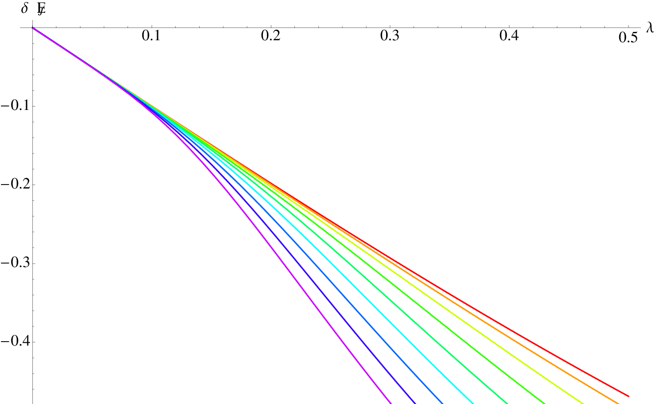
In the strong coupling limit , the energy goes to a constant value as
| (45) |
with being the logarithmic derivative of the function. This quantity is monotonous in the coupling and is plotted in Figure 3. Here, it should be noted that there exists a point at intermediate where the scaling with changes.

4 The entropy of the Majorana edge modes
In this section, we compute the entropy at of the MEMs and determine the dimension of the Hilbert space of the additional Majorana degrees of freedom localized at the concurring ends of the wires. We will compute the infinite-temperature limit of the entropy of the central region by looking at the asymptotic behaviour of the free energy of the localized Majorana modes, which in this limit is indeed dominated by the entropy and goes as .
In addition, we compute the entropy of the ground state for . The residual entropy found at zero temperature shows that the degrees of freedom introduced by the Majorana modes, are in a non-trivial superposition of degenerate states. We will obtain the entropy of the central region at from the first-order temperature correction to the free energy [45]
| (46) |
which in turn is obtained by substituting the zero-temperature solutions to the TBA systems (24) and (37).
Similarly to what observed in [50, 51], the systems (24) and (37) admit constant solutions [52, 53] both when and when . These solutions satisfy a set of coupled algebraic equations which we call “asymptotic” TBA. These are a simplified version of the TBA equations: we introduce them in section 4.1 for even and in section 4.4 for odd . Remarkably, the solution of this system can be parametrized in a similar way in the low- and in the high-temperature limits. Therefore, we will be able to study the high-temperature limit in sections 4.2 and 4.5 for even and for odd number of wires, respectively. We will also be able to study the low-temperature limit in sections 4.3 and 4.6, respectively for even and for odd values . The following sections will be devoted to the analysis of the TBA equations for even and odd number of branches.
4.1 The asymptotic TBA: even number of branches
Let us analyse the system (24): due to the boundedness of the source term, located in the equation for , the infinite temperature limit removes such term from the system. As a consequence, a constant solution appears. The presence of such solution, which only occurs in the limits of zero and at infinite temperature, greatly simplifies the analysis of the TBA equations. In fact, we plug such constant ansatz into (24) and rewrite the system in terms of the quantities
| (47) |
obtaining
| (48) |
It is implicit, here, that for . The solution of this system corresponds to the asymptotic value of the solution of the TBA equations at , when the source term disappears.
On the other hand, when the temperature goes to zero, the positive-defined driving term diverges to for all the values of the argument. As a result, it is possible to substitute another rapidity-independent ansatz into the TBA equations and one obtains once again the system (48), this time with the boundary condition
| (49) |
coming from the definition (47). On the contrary, at infinite temperature, since there are no divergences that can force one order of solutions to vanish, we expect for all values of and . Therefore, the very same set of algebraic equations (48) holds in the two regimes, high and low temperature, yet these regimes are distinguished by the boundary conditions (49) only.
Once we have the asymptotic solutions at infinite or at zero temperature, we insert them into the formula for the free energy (28). Then the constant asymptotic solution factors out of the integral, and one obtains that the temperature dependence of the free energy is given by
| (50) |
in which there appear the filling fractions
| (51) |
Note that (50) represents both the leading contribution to the free energy as and the first order correction in a low-temperature expansion. Of course, the asymptotic solutions for the s will be different in the two cases.
The solution to (48) is given in [53, 52] by the expression:
| (52) |
The quantities are objects which only depend on the overall symmetry of the problem and satisfy [54] the system of equations
| (53) | |||||
| (54) |
with initial conditions
| (55) |
It is understood that for all , as well as for all .
The expressions above are written in terms of sums of characters of the corresponding Lie algebra representations, each built on a given highest weight described in [53]. Such characters are specialized to the point , where is the Weyl vector, given by the sum of the fundamental weights The complex number is determined from the dual Coxeter number of the symmetry algebra ( for the algebra) and the positive integer ; the latter is the order at which the vanishing of the solution is imposed, as described below and in [53], and for the sake of definiteness it will be in the low-temperature limit and in the high-temperature limit.
4.2 The high temperature limit
Analogously to the results for the spin- Heisenberg spin chain and the multichannel Kondo model, we seek a rational solution to (48), which is non-vanishing for all the s. In particular, this is obtained when (or ). Then the characters appearing in (55) yield, by definition, the dimension of the representation of highest weight . In particular, we have:
| (57) |
By inserting such a solution into (55) and the latter into (56) we obtain the asymptotic fillings, corresponding to the solution at high temperature of the TBA system. These are explicitly listed in appendix A. By substituting these into (50) and evaluating it numerically for several values of , we conclude that
| (58) |
Note that, for , (58) yields the impurity entropy of the -channel Kondo model, while, for , the formula reproduces the impurity entropy of the Coqblin-Schrieffer model [45] with impurity in the fundamental representation. These correspondences are possible only if the dimension is the dimension of Majorana fermions projected to a definite fermion number parity sector. Indeed, four MEMs have a Hilbert space of dimension , while the Hilbert space of a localized spin- magnetic impurity, such as the one characterizing the two-channel Kondo model, only has dimension . The same reasoning applies to the case , for which the Hilbert space has dimension , corresponding to the dimension of the Hilbert space of six MEMs of given fermion number parity.
4.3 The low temperature limit
As observed earlier, at we need to solve (48) with the constraint (49). This is written in terms of the specialized characters of the irreducible representations of the algebra at the point , which corresponds to the choice in (55). These are provided in [54] as:
| (59) |
At this particular specialization, these three characters are enough [53] to determine the full solution recursively, thanks to the constraint (49), which implies the property , , , established in [53]. In fact, in (56), we only need the , . If , we can specialize the first of (53) for and, using , solve for . Analogously, we obtain recursively the results up to , which is most rapidly done by solving numerically the recurrence.
4.4 The asymptotic TBA: odd number of branches
In the same way as for even , the driving term disappears from the system (37) both in the high- and in the low-temperature limits. Therefore, the TBA system is reduced to:
| (61) | |||||
and the two regimes are distinguished by the fact that (49) has to be imposed at , while we have for all and all at . Note that for .
The solution to (61) is again given by (52), but now the s are solutions [54] of:
| (62) | |||||
with initial conditions given by
| (63) |
in which the dual Coxeter number is for the algebra.
The solution to (62), in turn, is provided in [53]. In order to evaluate the free energy, all we will be needing are the expressions:
| (64) | |||||
in which we note that only the numbers appear and they can be read in (63) once specialized to a particular value of . By using the definition (51) into the free energy (42), one obtains
| (65) |
for the junction free energy. This holds both as the leading order as and as the first order in a low- expansion, provided the corresponding asymptotic fillings are inserted.
4.5 The high temperature limit
We select the solution of (62) with in the initial values (63). Then, the specialized characters become – by definition – equal to the dimension of the corresponding representation. In particular:
| (66) |
Inserting such solutions into (64) we obtain the expressions listed in appendix A. Plugging them into (65) and evaluating numerically for several values of (odd) , we conclude that
| (67) |
for all odd values of ().
For , the dimension of the Hilbert space of four Majorana fermions with projection on a given fermion number parity sector is , the same as a for a localized spin- impurity such as the one characterizing the four-channel Kondo model. A related example has been addressed earlier in [55], who pointed out that, in a very similar setting, namely a junction of wires with three MEMs interacting among them, the Hamiltonian can be written in terms of Pauli matrices as well as in terms of operators satisfying (3). However, one expects to find inconsistency between the two operatorially equivalent formulations, in particular in the degeneracy of the spectrum. In fact, one can build a one-to-one correspondence between the Hilbert spaces only if the fermion number parity is considered.
4.6 The low temperature limit
As , we need to evaluate the solution of (61) with the constraint (49). Hence, we specialize the characters in (63) to the point , corresponding to in the initial values (63). From the expressions:
| (68) |
and rewriting the constraint (49) as , for and , as in [53], we can solve recursively the system (62). Once again, this is most efficiently done numerically. Evaluating the free energy of the MEMs by the use of (64) into (65) for several values of , we conclude that the ground state entropy produced by the topological Kondo term is
| (69) |
which shows that our thermodynamic Bethe ansatz agrees with the results of [32], obtained by boundary conformal field theory.
5 The specific heat of the Majorana edge modes
A signature of the non Fermi liquid nature of the strongly coupled fixed point is given by the next term in the expansion (46). In this section, we shall see that it is indeed of order . As a consequence, the Majorana contribution to the specific heat behaves at low temperatures as
| (70) |
where the (dimensionless) Kondo temperature depends on the coupling between legs as
| (71) |
A non-integer power is a strong and experimentally detectable signature of the presence of a non Fermi liquid fixed point. In particular, it is related to the operator content of the conformal field theory describing the fixed point at strong coupling, as explained in [39].
The power we find is indeed the same as what derived from the conformal dimension of the leading irrelevant operator in the conformal perturbation theory of [31] around the strongly coupled critical point. Therefore, we confirm such result from our Bethe ansatz computation. Also in this approach, it has its origin in the overall symmetry of the problem only, since what characterizes the Kondo model in the TBA equations, i.e., the functional form of the source term, disappears in the derivation of the -system. The latter is uniquely specified by the symmetry of the model, and the periodicity of the associated TBA equations is all we have used to determine the power characterizing the temperature dependence of the specific heat as .
5.1 Even number of branches
Following [45, 47], we focus on the rapidity regime , which introduces the first temperature corrections to the asymptotic values of the TBA functions. In fact, in this regime the source term is very small, being , so that the ratio with the temperature in the denominator gives a finite result and the rapidity dependence appears in the solution. For intermediate and large positive values of the rapidity, instead, the solutions of the TBA equations quickly approach their asymptotic zero-temperature value. It is convenient, in this regime, to shift the rapidities as , with .
Similarly to (47), we can define
| (72) |
and, starting from (24), we see that the s satisfy, for even and at low temperature, the following TBA system
| (73) | |||||
in which
| (74) |
and the only temperature dependence is the one implicit in the definition (72). The case is:
We now look at the free energy (28) and shift the integration variable as above. In order to express the temperature in terms of the Kondo temperature (71), we need to rescale the integration variable as , which brings its temperature dependence for into the form ()
| (75) |
In order to evaluate this expression, being the TBA equations (73) symmetric in the exchange , one only needs the functions
| (76) |
which come directly from the definitions (16) and (27). The case is again written as (75) with
| (77) |
Having already isolated the term in the free energy which is linear in the temperature, originating from the asymptotic value of the functions s, we now concentrate on the following term, which in turn comes from the low-temperature dependence on the rapidity of these functions.
Being the source term exponential and given the relation , a reasonable ansatz [56] is that, at low enough temperatures, the exponential behaviour of the source term is retained and we can assume the form
| (78) |
with being the already discussed asymptotic values. Under the ansatz (78), the free energy becomes
| (79) |
where the term linear in has been computed in section 4.1.
In order to fix the coefficient , we note that from the TBA systems (73) a universal -system for the analytic continuation in the complex plane of the functions can be derived, as explained in [57]. Universality, in this context, means that the source term of the integral equations disappear, i.e., that only the structure of the TBA is retained in the -system, while the source, characterizing the Kondo models, plays no role. We refer the reader to the original literature [57] for the explicit form of the -system and just state here that its solutions have periodicity:
| (80) |
which has been obtained in [58, 59] for both even and odd . It follows (see [60]) that they can be expanded in powers of the variable .
Substituting this expansion in the free energy (79) and using (70), we obtain that the specific heat of the MEMs vanishes at as the power law .
For , this value reproduces the results of [45] for the equivalent Coqblin-Schrieffer models.
5.2 Odd number of branches
We repeat here the procedure for an odd number of branches. After the change of variable we obtain, again at low temperatures and with the definitions (72) and (74), the TBA system
| (81) | |||||
The temperature dependence of the free energy for an odd number of legs and can then be rewritten as
| (82) | |||||
with the functions:
| (83) | |||||
As explained for even , substituting the ansatz (78) into (82), the free energy turns into
| (84) | |||||
whose linear term has been determined in section 4.4. This expression, using (70), proves that the specific heat vanishes as a power law of . The power itself is identified through the periodicity of the corresponding -system, as found in [58, 59]:
| (85) |
which proves that the power law is just the one stated in (70) and, therefore, that the system at the strong coupling fixed point cannot be modeled by a Fermi liquid.
For , this agrees with the known results for the four-channel Kondo model. We note in passing that the determination of a the specific heat characteristic power through the periodicity of the associated -system is, remarkably, more general than for the model considered. For instance, the formula , which can be proved from the periodicity properties assessed in [58] too, works in general for the classes of impurity models. In fact, for the -channel Kondo model, the level of the Bethe ansatz is , while the dual Coxeter number for is . Therefore , which is an elegant way of deriving an established result [43, 56, 39]. In the -species Coqblin-Schrieffer model, the dual Coxeter number is , hence the specific heat power law at low temperatures reads , as obtained in [45].
6 Concluding remarks
We have used the thermodynamic Bethe ansatz to provide an exhaustive analysis of the thermodynamics of the topological Kondo model. This model describes physical situations where external quantum wires concur in a central region, where the electrons interact with an extended “spin”, formed by spatially distant Majorana modes. The model has symmetry. Our study provided the thermodynamics of this model for arbitrary and a proof that this model represents a natural description of non-Fermi liquid quantum critical points associated with the Wess-Zumino-Witten-Novikov boundary conformal field theory. Indeed, a key result of our work is the exact computation of the low temperature behaviour of the specific heat of the central region. We have found that
where is the Kondo temperature and argued that the non-integer power originates only from the symmetry of the strong-coupling fixed point.
We have derived the exact free energy of the topological Kondo model and provided, in a closed form, the exact ground state energy shift due to the presence of the Majorana edge modes localized in the central region as a function of the effective interaction between the fermions in the external wires and the localized modes.
We have computed the entropy associated to the Majorana degrees of freedom localized in the central region – the so-called impurity entropy – both for and for . Our analysis provided the exact asymptotic expressions of the impurity entropy of the topological Kondo model for arbitrary .
For , the computation of the entropy determines the dimension of the Hilbert space associated to the Majorana edge modes localized in the central region and connected to the external wires. We found that the dimension of the Hilbert space corresponds to the Hilbert space of Majorana modes with projection to a definite fermion parity sector. This shows that it is always possible to preserve, for any given , fermion parity symmetry. Thus, conservation of the fermion number parity is an essential feature of the topological Kondo model.
Despite the topological Kondo Hamiltonian having been derived as an effective low-temperature model, at higher temperature, the topological Kondo effect is expected to survive as long as there are no processes breaking the fermion parity, e.g., single-electron tunnelling to or from the island, which become relevant.
Throughout this paper, we have assumed that the Majorana bound states in the central region were sufficiently separated in space so as to allow to neglect the direct coupling between pairs of Majorana modes. The inclusion of such terms should be an interesting extension of our work, since these terms are known to induce - for sufficiently low temperature - the crossover between different non Fermi liquid phases and could provide a signature of the presence of Majorana bound states in the central region.
Networks of quantum wires with Majorana edge modes realize the topological Kondo effect only when the superconducting central region is capacitively coupled with the ground [28, 29, 33, 34]; when the superconducting central region is floating, the system exhibits remarkable even-odd effect in the tunnelling conductance through the central region [30]. Both situations can be tested experimentally with present day technology, leading to the exciting possibility of an experimental test of exact results stemming from Bethe ansatz.
Ising spin chain realizations of the topological Kondo model have been also recently investigated in [36]. It was argued that this kind of system exhibits Fermi liquid behaviour at the strong-coupling fixed point when the number of legs is even, while it produces a non-Fermi liquid when the number of legs is odd. This feature, due to the reality of the fermions in the bulk, is manifest, e. g., in the low temperature behaviour of the specific heat and marks a difference with the model analysed in this paper, which reaches a non Fermi liquid fixed point at low temperatures for all values of .
Networks of chains could provide a basis for constructing alternative experimental realizations of the topological Kondo model investigated in this paper: their implementation could be realized in ultra-cold atom platforms and we think that it would be a very interesting line of future research to investigate feasibility and detection schemes in such setups.
Acknowledgements: We would like to thank N. Crampé, D. Cassettari, G. Dossena, R. Egger, A. Kuniba, A. Ferraz, A. Sedrakyan and A. Tsvelik for useful discussions and suggestions, as well as Nordita for hospitality during the program Quantum Engineering of States and Devices. The work has been carried on with the aid of the high performance computer system of the International Institute of Physics - UFRN, Natal, Brazil P.S. and F.B. acknowledge financial support from the Ministry of Science, Technology and Innovation of Brazil. P.S. thanks the Ministry of Science, Technology and Innovation of Brazil MCTI and UFRN/MEC for financial support and CNPq for granting a Bolsa de Produtividade em Pesquisa. V.K. is supported by the grant and H.B. acknowledges support from the Armenian grant and the Armenian-Russian grant . H.B. and V.K. are grateful to the International Institute of Physics of UFRN (Natal) for hospitality.
Appendix A Some explicit expressions for the asymptotic filling fractions
For the sake of clarity, we provide below the expressions for the first-order fillings at high temperature, which are connected with the solution of the TBA equations through (51), and give some more detail on the low-temperature asymptotic fillings as well. These directly follow from the procedure explained in section 4.
A.1 Even number of branches
At high temperature, as illustrated in the main text, we substitute the dimension of the fundamental highest-weight representations (57) into (55), thus obtaining all the for . Then we consider the system (53) with , which allows to compute all the for . Without any further iteration, we are provided an asymptotic high-temperature solution for the filling fractions by the use of (52). This solution is (56), which reads explicitly:
| (86) | |||||
Note that these values provide the occupation at high temperature of the real solutions of the Bethe equations by the use of (21).
The low-temperature limit is greatly simplified by the condition , , , discussed in section 4.3. In fact, we know from (55) and (59) and we can use it as an initial condition in order to start a numerical recursive solution of the system (53) with . In this way, we derive
| (87) |
and so on for , … , until having determined . We perform this recursion numerically. We already know from (55) and (59). By plugging the solution of this recurrence into (52), we obtain the asymptotic filling fractions.
A.2 Odd number of branches
In the high-temperature limit, we have all the for by substituting the dimension of the fundamental highest-weight representations (66) into (63). We now consider the system (62) with . This allows to compute all the for . Without any further effort, we can already compute all the for , by means of (52):
| (88) | |||||
In the low-temperature asymptotic limit, we know by means of (63) and (68). Moreover, we know that , , , as discussed in [58] and section 4.3. We can then use the system (62) with to set up a recurrence and determine numerically . The recurrence goes exactly as in the even- case and starts as:
| (89) |
and so on. We already know , again from (63) and (68). We substitute the solution of the procedure into (52) and obtain the desired asymptotic filling fractions .
References
- [1] T. Giamarchi. Quantum Physics in One Dimension. International Series of Monographs on Physics. Clarendon Press, 2003.
- [2] G. Morandi, P. Sodano, A. Tagliacozzo, and V. Tognetti. Field Theories for Low-Dimensional Condensed Matter Systems: Spin Systems and Strongly Correlated Electrons. Springer Series in Solid-State Sciences. Springer, 2000.
- [3] Philippe Di Francesco, P. Mathieu, and D. Senechal. Conformal Field Theory. Graduate Texts in Contemporary Physics. Springer, 1997.
- [4] V.E. Korepin, N.M. Bogoliubov, and A.G. Izergin. Quantum Inverse Scattering Method and Correlation Functions. Cambridge Monographs on Mathematical Physics. Cambridge University Press, 1997.
- [5] T.O. Wehling, A.M. Black-Schaffer, and A.V. Balatsky. Dirac materials. Advances in Physics, 63(1):1–76, 2014.
- [6] P. Schlottmann and P.D. Sacramento. Multichannel kondo problem and some applications. Advances in Physics, 42(6):641–682, 1993.
- [7] O. Houde, D. Kadio, and L. Pruvost. Cold atom beam splitter realized with two crossing dipole guides. Phys. Rev. Lett., 85:5543–5546, Dec 2000.
- [8] T. Schumm, S. Hofferberth, L. M. Andersson, S. Wildermuth, I. Groth, I. Bar-Joseph, J. Schmiedmayer, and P. Krüger. Observation of chiral currents with ultracold atoms in bosonic ladders. Nature Physics, 1:57–62, 2005.
- [9] D. Gallego, S. Hofferberth, T. Schumm, P. Krüger, and J. Schmiedmayer. Optical lattice on an atom chip. Opt. Lett., 34(22):3463–3465, Nov 2009.
- [10] G. L. Gattobigio, A. Couvert, G. Reinaudi, B. Georgeot, and D. Guéry-Odelin. Optically guided beam splitter for propagating matter waves. Phys. Rev. Lett., 109:030403, Jul 2012.
- [11] M. Atala, M. Aidelsburger, M. Lohse, J. T. Barreiro, B. Paredes, and I. Bloch. Observation of chiral currents with ultracold atoms in bosonic ladders. Nature Physics, 10:588–593, 2014.
- [12] K. Agarwal, E. G. Dalla Torre, B. Rauer, T. Langen, J. Schmiedmayer, and E. Demler. Chiral prethermalization in supersonically split condensates. arXiv:1402.6716, 2014.
- [13] C. Chamon, M. Oshikawa, and I. Affleck. Junctions of three quantum wires and the dissipative hofstadter model. Phys. Rev. Lett., 91:206403, Nov 2003.
- [14] M. Oshikawa, C. Chamon, and I. Affleck. Junctions of three quantum wires. Journal of Statistical Mechanics: Theory and Experiment, 2006(02):P02008, 2006.
- [15] A. Tokuno, M. Oshikawa, and E. Demler. Dynamics of one-dimensional bose liquids: Andreev-like reflection at junctions and the absence of the aharonov-bohm effect. Phys. Rev. Lett., 100:140402, Apr 2008.
- [16] K. Kazymyrenko and B. Doucot. Regular networks of Luttinger liquids. Phys. Rev. B, 71:075110, Feb 2005.
- [17] H. Guo and S. R. White. Density matrix renormalization group algorithms for y-junctions. Phys. Rev. B, 74:060401, Aug 2006.
- [18] I. Affleck. Quantum Impurity Problems in Condensed Matter Physics. ArXiv e-prints, sep 2008.
- [19] S. A. Reyes and A. M. Tsvelik. Crossed spin- heisenberg chains as a quantum impurity problem. Phys. Rev. Lett., 95:186404, Oct 2005.
- [20] D. Giuliano and P. Sodano. Y-junction of superconducting josephson chains. Nuclear Physics B, 811:395–419, apr 2009.
- [21] F. Wilczek. Majorana returns. Nature Physics, 5:614–618, 2009.
- [22] J. Alicea, Y. Oreg, G. Refael, F. von Oppen, and M. P. A. Fisher. Non-abelian statistics and topological quantum information processing in 1d wire networks. Nature, 446:167–171, 2007.
- [23] M.A. Nielsen and I.L. Chuang. Quantum Computation and Quantum Information. Cambridge Series on Information and the Natural Sciences. Cambridge University Press, 2000.
- [24] C. Nayak, S. Simon, A. Stern, M. Freedman, and S. Das Sarma. Non-abelian anyons and topological quantum computation. Rev. Mod. Phys., 80:1083–1159, Sep 2008.
- [25] A.M. Tsvelik. Topological Kondo effect in star junctions of Ising magnetic chains. Exact solution. New J.Phys., 16:033003, 2014.
- [26] N. Crampé and A. Trombettoni. Quantum spins on star graphs and the kondo model. Nuclear Physics B, 871(3):526 – 538, 2013.
- [27] R. M. Potok, I. G. Rau, Hadas Shtrikman, Yuval Oreg, and D. Goldhaber-Gordon. Observation of the two-channel kondo effect. Nature, 446:167–171, 2007.
- [28] B. Béri and N. R. Cooper. Topological kondo effect with majorana fermions. Phys. Rev. Lett., 109:156803, Oct 2012.
- [29] A. Altland and R. Egger. Multiterminal coulomb-majorana junction. Phys. Rev. Lett., 110:196401, May 2013.
- [30] A. Zazunov, P. Sodano, and R. Egger. Even-odd parity effects in majorana junctions. New Journal of Physics, 15(3):035033, 2013.
- [31] A. Altland, B. Beri, R. Egger, and A. M. Tsvelik. Majorana spin dynamics in the topological Kondo effect. Phys. Rev. Lett., (113):076401, 2014.
- [32] A. Altland, B. Béri, R. Egger, and A. M. Tsvelik. Bethe ansatz solution of the topological kondo model. Journal of Physics A: Mathematical and Theoretical, 47(26):265001, 2014.
- [33] B. Béri. Majorana-klein hybridization in topological superconductor junctions. Phys. Rev. Lett., 110:216803, May 2013.
- [34] A. Zazunov, A. Altland, and R. Egger. Transport properties of the coulomb-majorana junction. New Journal of Physics, 16(1):015010, 2014.
- [35] Gordon W. Semenoff and Pasquale Sodano. Stretching the electron as far as it will go. Electron.J.Theor.Phys., 10:157–190, 2006.
- [36] A M Tsvelik. Topological kondo effect in star junctions of ising magnetic chains: exact solution. New Journal of Physics, 16(3):033003, 2014.
- [37] I. Affleck. A Current Algebra Approach to the Kondo Effect. Nucl.Phys., B336:517, 1990.
- [38] I. Affleck and A.W.W. Ludwig. The Kondo effect, conformal field theory and fusion rules. Nucl.Phys., B352:849–862, 1991.
- [39] I. Affleck and A.W.W. Ludwig. Critical theory of overscreened kondo fixed points. Nuclear Physics B, 360(2-3):641 – 696, 1991.
- [40] Ian Affleck and Andreas W. W. Ludwig. Universal noninteger “ground-state degeneracy” in critical quantum systems. Phys. Rev. Lett., 67:161–164, Jul 1991.
- [41] E. Ogievetsky, N. Reshetikhin, and P. Wiegmann. The principal chiral field in two dimensions on classical lie algebras: The bethe-ansatz solution and factorized theory of scattering. Nuclear Physics B, 280(0):45 – 96, 1987.
- [42] H. J. De Vega and M. Karowski. Exact bethe ansatz solution of o(2n) symmetric theories. Nuclear Physics B, 280(0):225 – 254, 1987.
- [43] A.M. Tsvelick. The thermodynamics of multichannel kondo problem. Journal of Physics C: Solid State Physics, 18(1):159, 1985.
- [44] N. Andrei and C. Destri. Solution of the multichannel kondo problem. Phys. Rev. Lett., 52:364–367, Jan 1984.
- [45] A. Jerez, N. Andrei, and G. Zarand. Solution of the multichannel coqblin-schrieffer impurity model and application to multilevel systems. Phys. Rev. B, 58:3814–3841, Aug 1998.
- [46] A. Babichenko. From S matrices to the thermodynamic Bethe ansatz. Nucl.Phys., B697:481–512, 2004.
- [47] N. Andrei, K. Furuya, and J. H. Lowenstein. Solution of the kondo problem. Rev. Mod. Phys., 55:331–402, Apr 1983.
- [48] P. D. Sacramento and P. Schlottmann. Thermodynamics of the n-channel kondo model for general n and impurity spin s in a magnetic field. Journal of Physics: Condensed Matter, 3(48):9687, 1991.
- [49] M. Abramowitz and I.A. Stegun. Handbook of Mathematical Functions. Dover, New York, fifth edition, 1964.
- [50] H.M. Babujian. Exact solution of the isotropic heisenberg chain with arbitrary spins: Thermodynamics of the model. Nuclear Physics B, 215(3):317 – 336, 1983.
- [51] M. Takahashi. Thermodynamics of One-Dimensional Solvable Models. Cambridge University Press, 2005.
- [52] A. N. Kirillov and N. Yu Reshetikhin. Representation of yangians and multiplicities of occurrence of the irreducible components of the tensor product of representations of simple lie algebras. J. Phys. A, 20:1587, 1987.
- [53] A. Kuniba. Thermodynamics of the uq(xr(1)) bethe ansatz system with q a root of unity. Nuclear Physics B, 389(1):209 – 244, 1993.
- [54] A. N. Kirillov. Identities for the rogers dilogarithm function connected with simple lie algebras. J. Sov. Math., 47:2450, 1989.
- [55] Jaehoon Lee and Frank Wilczek. Algebra of majorana doubling. Phys. Rev. Lett., 111:226402, Nov 2013.
- [56] H.U. Desgranges. Thermodynamics of the n-channel kondo problem (numerical solution). Journal of Physics C: Solid State Physics, 18(28):5481, 1985.
- [57] A. Kuniba, T. Nakanishi, and J. Suzuki. T -systems and y -systems in integrable systems. Journal of Physics A: Mathematical and Theoretical, 44(10):103001, 2011.
- [58] A. Kuniba, T. Nakanishi, and J. Suzuki. Functional relations in solvable lattice models i: Functional relations and representation theory. International Journal of Modern Physics A, 09(30):5215–5266, 1994.
- [59] R. Inoue, O. Iyama, A. Kuniba, T. Nakanishi, and J. Suzuki. Periodicities of t-systems and y-systems. Nagoya Mathematical Journal, 197:59–174, 03 2010.
- [60] Al. B. Zamolodchikov. On the thermodynamic bethe ansatz equations for reflectionless ade scattering theories. Physics Letters B, 253(3):391–394, 1991.