UUITP-21/14
NSF-KITP-14-207
On the asymptotic states and the quantum S matrix of the -deformed superstring
Oluf Tang Engelunda and Radu Roibanb,c
a Department of Physics and Astronomy, Uppsala University,
SE-751 08 Uppsala, Sweden
oluf.engelund@physics.uu.se
b Department of Physics, The Pennsylvania State University,
University Park, PA 16802 , USA
radu@phys.psu.edu
c Kavli Institute for Theoretical Physics, University of California
Santa Barbara, CA 93106-4030 USA
Abstract
We investigate the worldsheet S matrix of string theory in -deformed . By computing the six-point tree-level S matrix we explicitly show that there is no particle production at this level, as required by the classical integrability of the theory. At one and two loops we show that integrability requires that the classical two-particle states be redefined in a non-local and -dependent way. This is a significant departure from the undeformed theory which is probably related to the quantum group symmetry of the worldsheet theory. We use generalized unitarity to carry out the loop calculations and identify a set of integrals that allow us to give a two-loop Feynman integral representation of the logarithmic terms of the two-loop S matrix. We finally also discuss aspects of the calculation of the two-loop rational terms.
1 Introduction
Integrability of the string sigma model is a key feature that makes possible the determination of the string spectrum on non-trivial curved backgrounds [1]. It is therefore important to identify and analyze such sigma models which correspond to physically-interesting string theories. Examples are integrable deformations of string sigma models on AdSSM10-2n which, in the undeformed case, play an important role in the AdS/CFT correspondence.
Orbifolding or sequences of T-duality (or worldsheet duality) and shift transformations (see e.g. [2, 3, 4, 5, 6]) of an integrable two-dimensional sigma model provide a straightforward way of constructing closely related integrable models. Generalizing previously-known constructions of integrable deformations of group or coset models [7, 8, 9, 10, 11, 12], a classically-integrable deformation of the AdSS5 Green-Schwarz sigma model was proposed in [13]. The deformation completely breaks target space supersymmetry and reduces the AdS5 and S5 isometries to their Cartan subgroups, UU. Remarkably however, the original symmetry is not completely lost but rather it is -deformed to PSU [14].
The bosonic Lagrangian was constructed explicitly and it was quantized in uniform light-cone gauge in ref. [15] (see [16] for lower-dimensional models and [17] for a discussion of the corresponding supergravity backgrounds); the bosonic tree-level S matrix was also constructed and shown to reproduce the small momentum (classical) limit of the PSU-symmetric S matrix of [18, 19, 20], suggesting that the gauge-fixed theory has indeed this symmetry. Integrability of the theory implies then that, if this symmetry is preserved at the quantum level, the S matrix should factorize as [21]
| (1) |
where each factor is invariant under a different PSU factor and may be written as
| (2) | ||||
Here is the part of the S matrix determined by the symmetries normalized such that the dressing phase is unity at tree level.
The small amount of manifest symmetry in this theory suggests that, by studying it, we may expose features that did not appear in the undeformed theory. For example, it is interesting to wonder whether integrability survives at higher orders and how is the PSU realized at the quantum level on the Lagrangian fields. The perturbative worldsheet S matrix is perhaps the most basic quantity which may help address these questions. We will compute it at tree-level beyond leading nontrivial S-matrix elements, as well as at one- and two-loop order. In doing so we shall also identify an integral basis which, in conjunction with generalized unitarity, yields a Feynman integral representation for all the logarithmic terms in the two-loop S matrix. The construction of this basis may be iterated to all loop orders.
An important property of higher-point S matrices in integrable theories is the absence of particle production or, alternatively, their factorization of the (tree-level) higher-point S matrix into sequences of processes [21]. This feature has important simplifying consequences on the unitarity-based construction of the S matrices of such theories [22, 23, 24]. As we shall review in sec. 3.1, it implies the cancellation of massive tadpole integral contributions to the 1PI part of the S matrix and thus suggests that, if present, UV divergences are confined to the renormalization of two-point functions.
It was pointed out in [25] that, for an S matrix to have desirable properties, one should in principle allow for transformations of the multi-particle scattering basis, which from the point of view of the constituent one-particle states appears mutually non-local. These transformations may significantly modify the symmetry properties of the S matrix without changing the actual physical content. As we shall see, such a bilocal transformation (in momentum space) is necessary in the -deformed theory to put the loop-level S matrix in the form (2) suggested by the integrability and classical symmetries of the theory. One may, alternatively, interpret the required transformation as acting on single-particle states at the expense of changing their dimension and spin, both of which become formally complex. The necessity for this redefinition is a significant departure from the undeformed theory11 1 In the undeformed theory a redefinition of creation/annihilation operators is necessary to relate the worldsheet and spin chain S matrices, see [25]. and appears to be closely related to the presence of an NS-NS field and the corresponding bosonic Wess-Zumino term. However, the presence of such a field does not necessarily require such redefinition as shown by loop calculations in AdSST4 supported by mixed flux [26, 27]. It therefore seems likely that it is required for the naive tree-level asymptotic states to become a representation of .
In general, to carry out loop calculations it is necessary to know the interaction terms containing worldsheet fermions. As we shall see however, part of our conclusions can be reached based only on the structure of the S matrix and with minimal detailed information on the fermion-dependent part of the Lagrangian or of the corresponding S-matrix elements. When we derive explicit expressions of loop-level S matrix we shall use for the currently-unknown tree-level S matrix the relevant terms in the small momentum expansion of the S matrix of [18, 19, 20].
The paper is organized as follows. In sec. 2 we review the deformed Lagrangian and its bosonic part, the structure of the four-particle S matrix and discuss the factorization of the six-particle S matrix. In sec. 3 we construct the one-loop S matrix in terms of the tree-level S-matrix coefficients and identify the redefinition of the two-particle states that cast it in the form suggested by the classical symmetries and integrability. In sec. 4 we describe a new basis of two-loop integrals, give an integral representation of the logarithmic terms of the two-loop S matrix and provide a discussion of the rational terms. In sec. 5 we summarize our results and discuss how to construct an integral representation for the worldsheet S matrix at arbitrary loop order. We relegate to appendices explicit expressions for the tree-level S-matrix coefficients, one-loop integral coefficients and one-loop S-matrix coefficients and explicit expressions for one- and two-loop integrals.
2 The deformed action and bosonic Lagrangian
The one-parameter -deformation of the AdSS5 supercoset Lagrangian constructed in [13] is naturally expressed in terms of the left-invariant one-forms of the undeformed symmetry group:
| (3) | |||
| (4) |
Here PSU and are projectors onto subspaces with eigenvalue of the action of the automorphism of PSU.22 2 We use the normalization in which the (super)trace of squares of the bosonic Cartan generators equals 2. The operator acts on the superalgebra as
| (5) |
where the operator multiplies the generators corresponding to the positive roots by , those corresponding to the negative roots by and annihilates the Cartan generators. There are three choices of operator leading to inequivalent bosonic actions (the corresponding metrics appear to have different singularity structures) [14].
The Lagrangian (4) has several remarkable properties. On the one hand it preserves the classical integrability of the undeformed theory. On the other, it exhibits a -deformed symmetry [14], which suggests that the theory is more symmetric than manifest from the Lagrangian. The parameter is related to the deformation parameter as
| (6) |
This relation was initially inferred in [15] by comparing the tree-level S matrix of the deformed model with the PSU-invariant S matrix of [18, 19, 20]. Up to the normalization of the worldsheet action (and hence of ), the same expression was found in [14] where the symmetries of the classical action have been analyzed.
2.1 The bosonic Lagrangian and the four-point S matrix
Using the choice of operator put forth in [13] and a judicious parameterization of the coset, the bosonic Lagrangian was constructed in [15]. Unlike the undeformed theory, the geometric background is supplemented by a nontrivial NSNS B-field. The Lagrangian is:
| (7) |
with33 3 The relation between and is .
| (8) | |||||
| (9) | |||||
and the Wess-Zumino terms and given by
| (10) | |||||
| (11) |
The light-cone gauge-fixing of this Lagrangian was discussed at length in [15] and we will not reproduce it here. For the purpose of the construction of the S matrix it is useful to pass to complex coordinates, which manifest the SU in the limit. Restricting to the fields the transformation is
| (12) | |||
The Lagrangian to quadratic and quartic orders (, etc) is then44 4 These expressions are obtained by Legendre-transforming the Hamiltonian of [15]. Alternative expressions may be obtained by expanding the Nambu-Goto action.
| (13) | ||||
| (14) | ||||
| (15) | ||||
| (16) |
Remarkably, the bosonic tree-level four-point S matrix given by this Lagrangian reproduces [15] the small momentum limit of the exact PSU-invariant S matrix of [18, 19, 20].
In secs. 3 and 4 we shall need the general form of the two-particle S matrix. Based on the manifest and expected symmetries the general form of the -matrix elements in (2) is:
| (17) |
The tree-level values of the coefficients of the bosonic structures, , have been constructed directly from the Lagrangian in [15]. At this order
| (18) |
their common value corresponds to the contribution of the Wess-Zumino term and it does not depend on the particle momenta. In Appendix A we collect the tree-level expressions of all coefficients in (17) extracted from [18, 19, 20] by taking the small momentum expansion.
2.2 Six-point S matrix and absence of particle production
One of the consequences of integrability is the absence of particle production or, alternatively, the factorization of the S matrix into a sequence of scattering events [21]; all possible factorizations are equivalent as a consequence of the Yang-Baxter equation obeyed by the four-particle S matrix. Here we discuss the absence of tree-level scattering processes for the -deformed worldsheet theory and the corresponding factorization of the tree-level amplitude. This calculation verifies the classical integrability of the gauge-fixed theory and, moreover, is an integral part of the unitarity-based approach to the construction of the S matrix in integrable quantum field theories.
For the purpose of illustration we will focus here on the fields parametrizing S5. It is straightforward, albeit tedious, to expand the parity-even part of the gauge-fixed deformed Lagrangian to this order. It is however simplest to check the factorization of the parity-odd part of the (bosonic) S matrix. Indeed, these matrix elements depend only of the parity-odd six-field terms in the expansion of the Lagrangian (and lower order terms as well) which are substantially simpler. In the notation of [15], they are given by:
| (19) |
The propagator coming from the quadratic Lagrangian is of the form
| (20) |
for some choice of and . The Feynman rules from the quartic Lagrangian (15)-(16) are
![[Uncaptioned image]](1412.5256v2/4pt_t1.png) |
(21) | |||
![[Uncaptioned image]](1412.5256v2/4pt_t2.png) |
(22) | |||
for some choices of the constant coefficients and which may be easily found by inspecting eqs. (15)-(16).
We will consider explicitly the process with incoming fields and with momenta and , respectively; for the outgoing fields we will take two s (with momenta and ) and two s (with momenta and ). The relevant Feynman graph topologies are shown in fig. 1. The graph of type fig. 1 appears four times, where the outgoing leg with momentum can be assigned to any one of the outgoing fields. The graph of type fig. 1 appears in principle six times, with the outgoing legs with momenta being assigned to all possible pairs of momenta; due to our choice of flavor of outgoing fields however, two of such assignments ( and ) vanish identically.

Straightforward algebra shows that upon using the identity
| (23) | ||||
| (24) |
and combining the eight contributions all propagators cancel out and we find a local expression. For all choices of and coefficients in (22) it can be put into a form reminiscent of the contribution of a six-point vertex:
| (26) | |||||
It is not difficult to check that such a six-point vertex Feynman rule arises from the second term in the parity-odd six-field Wess-Zumino term in eq. (19). We have also checked that the same is true for all parity-even and parity-odd six-point tree-level S-matrix elements.
3 The one-loop S matrix
A direct calculation of the one-loop S matrix is interesting for several reasons. On the one hand it would probe the integrability of the theory beyond classical level and it would determine to this order the dressing phase of the S matrix (in the small momentum expansion). On the other it would explore the realization of symmetries at the quantum level and the extent to which the classical asymptotic states form a representation of the symmetry group assumed in the construction of the exact S matrix [18, 19, 20]. Should the two realizations be different, an explicit expression of the S matrix in terms of classical asymptotic states would allow us to determine the (nonlocal) redefinition that relates them to the true one-loop (and perhaps all-loop) states. We will denote henceforth this S matrix (and the corresponding matrix) with the index ””.
In the following we will use unitarity-based methods [28, 29] discussed in the context of two-dimensional integrable theories in [22, 23, 24] to find the one-loop and the logarithmic terms of the two-loop S matrix. This construction will assume that the asymptotic states are the classical ones, with two-particle states realized as the tensor product of single-particle states.
An important ingredient in the construction of the S matrix through such methods are the tree-level S-matrix elements with fermionic external states, which are currently unknown from worldsheet methods. As we shall see, to draw conclusions on the properties of asymptotic states only the general form of the tree-level S matrix and general properties of the tree-level coefficients (which may be justified by e.g. assuming integrability) are necessary. To find the actual expression of the loop-level S matrix we shall extract the tree-level fermionic S-matrix elements from the exact S matrix.
3.1 Comments on unitarity vs. Feynman rules
The construction of scattering matrices in two-dimensional integrable models from unitarity cuts was discussed in detail in [22], [23]. While in [23] only the terms with logarithmic momentum dependence were discussed, ref. [22] gave a prescription the calculation of the complete one-loop S matrix; it is interesting to discuss its relation to the Feynman diagram calculation in [30] or the analogous calculation in the -deformed theory.
As discussed in [30] in the context of undeformed AdSSn theories, the off-shell one-loop two-point function vanishes on shell. Moreover, the one-loop four-point function is also divergent and the on-shell divergence is proportional to the tree-level S matrix. The corresponding renormalization factors necessary to remove all divergences are related to each other and can be simultaneously eliminated by a field redefinition. One may understand the relation between renormalization factors as a consequence of the (spontaneously broken) scale invariance of the theory. Due to integrability, the unitarity-based calculation [22], [23] is insensitive to the second type of divergence, which would correct the four-point interactions. Indeed, integrability in the form of the factorization of the six-particle amplitude implies that a one-particle cut of the one-loop four-point amplitude, which would identify the divergent tadpole integral, contains a further cut propagator and that it is in fact a two-particle cut and thus it predicts the absence of an infinite renormalization of the four-point vertex. This is consistent with the fact that the one-particle cut of the on-shell two-point function computed from the four-point S matrix vanishes as well. Thus, on the one hand, Feynman graph calculations exhibit divergences removable by field redefinitions while unitarity-based calculations are insensitive to any such divergences.
Before embarking in the unitarity-based construction of the one-loop S matrix for the -deformed theory, it is useful to check whether a similar consistent setup exists in this case as well. This is indeed the case. In the previous section we illustrated the fact that the six-point tree-level S matrix factorizes and thus the one-particle irreducible contributions to the one-loop four-point S matrix are free of tadpole integrals. One can also check using the tree-level four-point S matrix (17) with coefficients given in Appendix A that the one-particle cut of the on-shell one-loop two-point function vanishes as well. Assuming that the worldsheet theory has indeed spontaneously-broken scale invariance (as it should to be a good worldsheet theory expanded around a nontrivial vacuum state) and by analogy with the undeformed case, we may therefore expect that unitarity-based calculation as described in [22], [23] will capture the complete one-loop S matrix.
3.2 One-loop logarithmic terms and the need for new asymptotic states
To understand whether corrections to asymptotic states are necessary, let us first construct the logarithmic terms of the one-loop S matrix under the standard assumption that the loop-level asymptotic states are the same as the tree-level ones and contrast the results with the consequences of integrability (2).


To this end we use the unitarity-based method described in two-dimensional context in [22, 23, 24]. The one-loop S matrix with tree-level asymptotic states (denoted by the lower index ) is given by
| (27) |
where the integrals are shown in fig. 2. We used their values for the propagators following from the action (14), and the -channel integral was defined through Wick rotation to Euclidean space. The integral coefficients , and are determined by unitarity cuts, with a suitable interpretation55 5 To extract the coefficient of the -channel one notices that on the one hand the formal cut of the -channel integral is divergent due to the squared propagator and on the other the cut evaluated as a product of tree-level amplitudes is also divergent due to the momentum conserving delta function. The prescription of [22] is to identify the coefficients of these divergences in the limit in which the cut momentum equals one of the external momenta. of the singular -channel cut:
| (28) | |||||
| (29) | |||||
| (30) | |||||
Since the unitarity cuts fix completely the loop momentum, it is convenient to express the one-loop amplitude in terms of (the tree-level part of the) the coefficients parameterizing the S matrix, cf. eq. (17). The Grassmann parity of states introduces relative signs between various contributions; to keep track of them it is convenient to introduce the parameter with defined as
| (31) |
The components of the difference between the - and -channel integral coefficients,
| (32) |
expressed in terms of generic tree-level S-matrix coefficients in eq. (17) are collected in Appendix C. These expressions contain a variety of terms whose structure is different from that expected of the tensor part of the S matrix on the basis of integrability and factorized symmetry. Assuming that the symmetry generators receive corrections, the only terms that may become consistent with symmetries are those proportional to the tree-level S matrix. Not all such terms survive however due to the identities
| (33) |
which may be found using the expressions for the bosonic tree-level S-matrix elements found in [15]. The terms that are not proportional to the tree-level S matrix must cancel; this requires that the following relation must hold:
| (34) |
Showing that this holds requires knowledge of fermionic S-matrix elements. We extracted them from the exact S matrix of [18, 19, 20]. Even though they have not yet been found through direct worldsheet calculations, the fact that the sigma model is classically integrable [13] and has PSU quantum group symmetry [14] suggests that they should be the correct ones.
Using these identities, eqs. (79)-(86) can be compactly written as:
| (35) |
Thus, it follows that the logarithmic terms of the one-loop S matrix with tree-level asymptotic states are given by
| (36) |
We note that the first line of this expression is inconsistent with the expansion (2) of the S matrix suggested by quantum integrability and the expected PSU symmetry. Indeed, eq. (2) implies that at one-loop level the only logarithmic momentum dependence appears in the S matrix phase – and thus the only logarithms multiply the unit operator – while the tensor part is free of logarithms.
3.3 One-loop symmetries and new asymptotic two-particle states
The fact that the offending term in eq. (36) is proportional to the tree-level S matrix suggests that it should be possible to eliminate it by a redefinition of the asymptotic states. At tree level these states are tensor product of single-particle states however this does not need to be the case at loop level. We will consider two redefinitions: one makes the spin and dimension of the single-particle states complex while preserving the tensor-product structure of the two-particle state and the other does not act independently on the single-particle states but breaks the tensor product of the two-particle states. While distinct, the two redefinitions have the same effect on the S matrix and put it in a form consistent with the consequences of integrability and expected symmetries.
To identify the desired transformation we notice that for all choices of external states the following identity holds:
| (37) |
For diagonal elements, and , both the left-hand and the right-hand side are trivially zero, while they are non-vanishing for off-diagonal S-matrix elements. Using this identity, the two possible redefinitions are:
| (38) | |||||
| (39) |
Since the tree-level coefficient is purely imaginary, , cf. eq. (18), both redefinitions preserve the unitarity properties of the original S matrix as the in and out states remain hermitian conjugates of each other. We also notice that the redefinition is not sensitive to the order of the states in the original tensor product. Of course, at one loop only the first term in the expansion of the exponential factors is relevant; we however keep the full exponential form to exhibit manifest unitarity of the state transformation.
In terms of the new asymptotic states and upon using eq. (37) the one-loop S matrix becomes
| (40) |
by construction the logarithmic terms proportional to cancel in the parenthesis and we are left with an expression consistent with integrability and expected symmetries. In the limit of vanishing deformation parameter, , the bare and redefined states become identical, as required by the fact that no state redefinition is necessary in the undeformed theory.
Following [22], the -channel integral coefficient can be found by removing the vanishing Jacobian factor from the tree-level S matrix, eq. (30), and is given by:
| (41) |
In the limit of zero deformation this coefficient gives rise to the rational part of the one-loop dressing phase whereas gives the one-loop terms in the expansion of the coefficients in the definition (17) of the S matrix.66 6 In theories with cubic interaction terms there may exist nontrivial corrections to the two-point function of fields which change its residue at the physical pole. This leads to further terms in the one-loop S matrix, see [24]. The -deformed AdSS5 Lagrangian has only quartic (and higher-point) vertices and thus such corrections appear only at two loops. For non-vanishing -parameter we have checked that this continues to be the case by comparing the entries of with the perturbative expansion of the exact S-matrix coefficients [18, 19, 20]. We collect the expressions of the one-loop S-matrix coefficients in Appendix D.
4 The two-loop S matrix and consistency of the asymptotic states
In [23] the double-logarithms of the two-loop S matrix were computed from double two-particle cuts and expressed in terms of two-loop scalar integrals. Additional single-logarithms were then found from single two-particle cuts, making use of the rational part of the one-loop S matrix determined by symmetries 77 7 The part proportional to the identity operator cancelled out.. The result was, however, expressed only in terms of one-loop integrals. Here we identify a particular set of two-loop scalar and tensor integrals which allows us to write a uniform two-loop integral representation of all two-loop logarithmic terms.
4.1 A set of tensor integrals
The topologies of the contributing integrals are the same as in [23] and are shown in fig. 4. Let us parametrize the integrals in figures 4, , and as shown in the figure. We first consider the cut in the channel, which receives contributions from graphs with topologies , and . If one interprets them as scalar integrals, then the two-particle cut condition for the graph has two solutions both of which are proportional to the -channel one-loop integral. The two particle cut conditions of graphs and also have two solutions; however, one of them is proportional to the -channel one-loop integral while the other is proportional to the -channel one; the corresponding solutions may be parameterized as
| (42) |
Instead of using them however, we shall define integrals whose single two-particle cuts receive contributions from a single one-loop integral. This can be easily done by making use of the solution (42) to the cut condition and inserting appropriate momentum-dependent numerator factors. Denoting by the denominator of the products of scalar propagators corresponding to the graphs in fig. 4, they are
| (43) | |||||
| (44) | |||||
| (45) |
where
| (46) | ||||||
| (47) |
The -channel two-particle cut of the integrals and receives contributions only from -channel one-loop sub-integrals, the -channel two-particle cut of the integrals and receives contributions only from -channel one-loop sub-integrals while the two-particle cuts of the remaining integrals receive contributions only from the -channel one-loop sub-integrals.
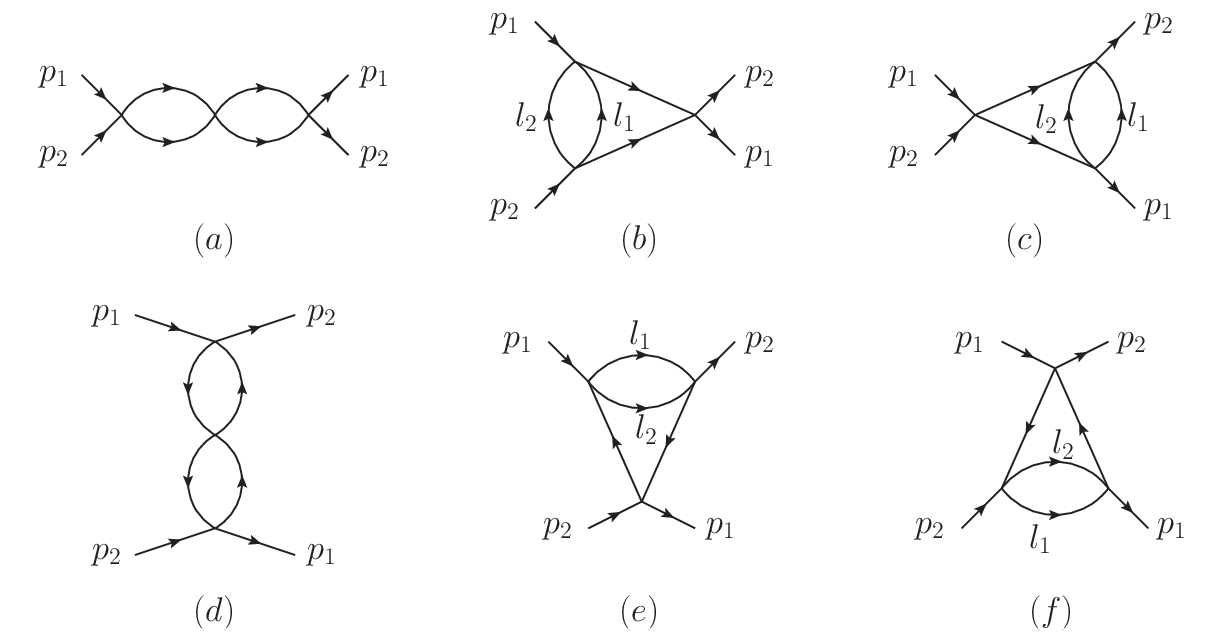
In terms of the ten scalar and tensor integrals , the ansatz for the logarithmic terms of the two-loop S matrix is
| (48) | ||||
| (49) |
using the explicit expressions for the integrals listed in Appendix E it is not difficult to see that may be written as
| (50) | ||||
The ten coefficients are determined by single two-particle cuts in terms of tree-level amplitudes and one-loop integral coefficients , and . Each solution to the cut condition determines exactly one coefficient. The first six coefficients have the same expression as the coefficients with the same name in ref. [23],
| (51) |
while , , and are given by
| (52) | ||||
Since the coefficient of the one-loop logarithms depends only on the differences (cf. eq. (27)), the coefficient of the two-loop double-logarithm should have a similar property. As discussed in the previous section, this difference has two parts; one proportional to the identity operator and one proportional to the tree-level S matrix. It is not difficult to check that the part proportional to the identity operator cancels out in the two-loop S matrix; the remaining bilinear in tree-level S-matrix elements can again be organized in terms of the difference . Upon using the identity
| (53) |
the coefficient of the double-logarithm becomes proportional to the tree-level S matrix, and may be suggestively organized as
| (54) |
To find the coefficient of the simple logarithms we first recall [23] that, on general grounds related to the consistency of single and double two-particle cuts of two-loop S-matrix elements, the contribution of terms proportional to the identity operator in the one-loop S matrix vanishes. Using eq. (53) we find that, up to rational terms, the two-loop S matrix is given by
| (55) | ||||
As in the case of the one-loop S matrix, this expression is not immediately consistent with the implications of symmetries and integrability (2). Using however the one-loop corrected asymptotic states, all offending terms cancel out and we find
| (56) |
This is indeed the expected structure of the two-loop S matrix. Thus, the exponentiation of the one-loop redefinition of the asymptotic states (38), (39) does not receive further two-loop corrections. It is natural to conjecture that the same holds at higher loops as well; it would, of course, be interesting to verify whether this is indeed the case.
4.2 Comments on rational terms
The combination of two-loop integrals (48) giving the correct single and double-logarithms also contains some rational terms originating from the rational terms in the expressions of the two-loop integrals (108). By construction however, these terms do not account for all the possible two-particle cuts of the two-loop S matrix, in particular the cuts in which there is no net momentum flow across it, which are analogous to the one-loop -channel cut; the potentially missing relevant integral topologies are shown in fig. 5. As in that case, one can convince oneself that all integrals based on these graphs are momentum independent (and thus their cuts are to be understood in a formal sense) and consequently they can contribute only rational terms to the two-loop S matrix. A further source of rational terms are the quantum corrections to the off-shell two-point function and additional integrals that have only -channel two-particle cuts.

The first corrections to the two-point function of fields arise from Feynman graphs of topology 88 8 In principle there are also graphs containing tadpoles, but they should cancel out and the final contribution arises effectively only from the topology in fig. 6.99 9 The fact that the first correction appears at two-loop level follows from the absence of cubic vertices in the gauge-fixed Lagrangian. In theories where such cubic vertices are present the first correction appears already at one loop, see e.g. [24]. shown in fig. 6 and change the residue of the propagator at the physical pole; this must be accounted for in the definition of the S matrix. Since the first correction to the dispersion relation arises at two-loop order, the additional terms in the two-loop S matrix are necessarily proportional to the tree-level S matrix.
In the following we will not determine all rational terms; rather, we will point out specific features which appear to suggest how they can be found through generalized unitarity. We begin by pointing out an interesting property of the calculation of the two-loop S matrix [31] in the near-flat space limit [32] of AdSS5. In this limit all integrals with the topology in fig. 5(a) have vanishing coefficients, while the integrals with the topology in figs. 5(b) and 5(c) exactly cancel the quantum corrections to the external states. We will attempt to show that a similar pattern may be realized in general; we will also see that for this to happen it is necessary that the integral representation of the two-loop S matrix contains integrals that do not have two-particle cuts.

Since, as mentioned earlier, the two-loop corrections to the two-point function contribute to the two-loop S matrix terms proportional to the tree-level S matrix, to check the fate of these terms we shall focus on the integral coefficients corresponding to the topologies shown in fig. 5 which are also proportional to the tree-level S matrix. There are six combinations of tree-level S-matrix elements and one-loop integral coefficients which can appear in two-particle cuts (and thus determine these integrals’ coefficients) and have this property:
| (57) | ||||
It is not difficult to identify these combinations as contributions to two-particle cuts from a single solution to the cut condition. The other solutions contribute terms proportional to the identity matrix and, while important for the complete S matrix (in particular for the determination of the complete two-loop dressing phase) will ignored in the following. The numerator factors which can be used to dress the graphs in fig. 5 and select the desired solution to the two-particle cut condition such that the resulting integrals have as coefficients are:
| (58) | ||||
Then, denoting as before by the denominators of scalar propagators associated to the graphs in fig. 5, the integrals whose coefficients are given by eqs. (57) are1010 10 The reader may notice that the systematic for generalizing the one-loop cuts to two-loop cuts seems to have been flipped around for the -channel. This is indeed the case as a careful analysis along the lines of [22] will show. :
| (59) | ||||||||
We choose to use light-like directions in the numerator factors only for convenience, the resulting integrals having been already computed in [31]; a different choice would lead to different values for the integrals. It is not surprising that different numerator factors are possible: indeed, by expressing all loop momenta in terms of external momenta in two dimensions, cuts cannot determine unambiguously the tensor structure of an integral. Interestingly, the coefficients are such that when the component of the loop momenta used to construct the numerator is changed, the extra terms in the two-loop S matrix are proportional to the scalar sunset integral, see fig. 6.
To compute the corrections to external states the off-shell two-point function is necessary, because the residue of the corrected propagator contains the derivative of the two-point function with respect to the worldsheet energy. We shall assume that this derivative is entirely given by the derivative of the integral. With this assumption we shall construct the two-point function by sewing two legs of the one-loop S matrix. There are four possible index contractions:
| (60) |
which are the direct two-loop generalizations of the one-loop contractions
| (61) |
which indicate the absence of external line tadpoles in the one-loop S matrix.
The contractions are coefficients of integrals with the topology given in fig. (6) whose one-particle cuts localize on a single solution of the cut condition. Denoting by and the denominators of the product of scalar propagators corresponding to the graph fig. (6) with external momentum and , respectively, the numerator factors that lead to the desired localization are
| (62) |
and lead to the integrals
| (63) |
It turns out that the result also depends on the scalar sunset integral; we shall denote this integral by
| (64) |
Putting all this together the several contributions, we get that the additional rational terms proportional to the tree-level S matrix not already present in (50) can be written as
| (65) | ||||
| (66) |
where the primes indicate derivative with respect to the time-like component of the external momentum.
It is straightforward to calculate all the integral coefficients. We find that impliying that, similarly with the near-flat space calculation [31], the two-point function depends only on integrals of wineglass topology. As some of the non-zero coefficients are equal the results can be written in terms of integrals simpler than the integrals in the basis, the useful combinations are collected in appendix E. The result can be written as:
| (67) |
We have not explicitly written out the function because it can be changed by changing the momentum components used in the numerators in (58). We notice that the remaining term is proportional to the integral which is associated with topologies of the type shown in fig. 7. Even though is constant, this is not a vacuous statement: while we have not determined the the fact that the S matrix can in principle be computed using Feynman rules implies that this function should not contain factors of . One may remove such a contribution by adding to the ansatz (65) further terms based on the integral in fig. 7. Adding such terms may also be used to repair e.g. a potential lack of factorization of the three-particle cuts of the ansatz in (48).

In addition to the potential cancellation described above, which mirrors the pattens of the undeformed near-flat space calculation, it is useful to also note the different dependence on the Jacobian factor of the integrals in figs. 5 and 6 and fig. 4. The fact that the former integrals depend on a single external momentum implies that, unlike the latter integrals, their expression cannot contain any factors of . This suggests that integrals having two-particle -channel cuts contribute to parts of the two-loop S matrix that are distinct from those that receive contributions from integrals having - and -channel cuts.1111 11 This statement ignores potential factors that may exist in the integral coefficients. In turn this observation implies that the rational part of the one-loop dressing phase (contributing to the two-loop S matrix multiplied by the tree-level S matrix, cf. eq. (2)) should be present in the terms written explicitly in equation (50). This is in fact the case: the last line of that equation is
| (68) |
which indeed reproduces the contribution of the rational part of the one-loop dressing phase to the two-loop S matrix, cf. eq. (2) and the discussion in sec. 3.3, eqs. (40) and (41).
5 Discussion
In this paper we discussed in detail string theory in -deformed AdSS5 and we have seen that, for the perturbative worldsheet S matrix to be consistent with integrability and the expected PSU of the gauge-fixed theory the naive tree-level two-particle asymptotic states (and more generally all multi-particle asymptotic states) must be redefined non-locally. We have checked that the exponentiation of the redefinition required by the one-loop S matrix renders consistent the two-loop S matrix as well suggesting that this exponentiation may be exact to all loop orders. It would of course be interesting to check whether this is indeed the case.
The necessity for such a redefinition, which does not parallel the undeformed theory, is related to the presence of the deformation and in particular to the fact that the worldsheet theory contains a nontrivial bosonic Wess-Zumino term. Since the worldsheet symmetry generators have a nontrivial expansion around the BMN vacuum, it is possible that the redefinition we identified is necessary for the two-particle state to be a representation of the PSU symmetry of the gauge-fixed theory at the quantum level. It would be interesting to explore the properties that a nontrivial NS-NS background should have for such a redefinition to be necessary.
We have also identified a set of two-loop scalar and tensor integrals that capture all the logarithmic terms in the two-loop S matrix. By evaluating the integrals we have observed that the same expression also captures correctly some rational terms, in particular the rational terms corresponding to the contribution of the one-loop dressing phase to the two-loop S matrix. Other such terms however are not; attempting to understand them we pointed out that a certain cancellation pattern between external line corrections and -channel integrals can occur provided that one allows for the presence of integrals that have only three-particle cuts. It goes without saying that a complete understanding of the rational terms of the two- and higher-loop S matrix remains an important open problem.
Ideally, one would expect that, to any loop order, it should be possible to write an integral representation for the S matrix of the form
| (69) |
where are integrals with only four-point vertices, are cuts written entirely in terms of the four-point tree-level S matrix and are symmetry factors of the corresponding integrals. There is a certain amount of freedom in choosing the integrals and not all choices need to be consistent with integrability, in particular the fact that cuts isolating tree-level higher-point amplitudes are factorized. Thus, apart from the integrals listed above, tree-level integrability may require inclusion of integrals with higher-point vertices as well.
With the appropriate definition of propagators, the integrals identified here can be used to construct the massive S matrix in all AdSSM10-2n spaces and, presumably, in all two-dimensional integrable theories. For however an important issue that awaits a satisfactory resolution is the contribution of massless modes. It has been suggested in [24] and verified explicitly in [30] through Feynman graph calculation that they do not contribute to the S matrix at one-loop level. It would be interesting to understand the reason behind this feature and whether their decoupling continues at higher loops as well.
Acknowledgements:
We would like to thank S. Frolov, B. Hoare and A. Tseytlin for useful discussions and B. Hoare, J. Minahan and A. Tseytlin for comments on the draft. RR acknowledges the hospitality of the KITP at UC Santa Barbara and, while this work was being written up, also that of the Simons Center for Geometry and Physics. The work of OTE is supported by the Knut and Alice Wallenberg Foundation under grant KAW 2013.0235. The work of RR was supported in part by the US Department of Energy under contract DE-SC0008745 and while at KITP also by the National Science Foundation under Grant No. NSF PHY11-25915.
Appendix A Tree-level S-matrix coefficients
In this appendix we collect the tree-level expressions of the coefficients of the various tensor structures parametrizing the S matrix, see eq. (17):
| (70) | ||||
Appendix B Dispersion relation, propagator and Jacobian
The deformation changes the dispersion relation which in turn affects our calculations in numerous different ways. In this appendix we include some of the affected quantities as well as some useful identities. The dispersion relation to leading order in the large expansion is:
| (71) |
From this it is not hard to show that
| (72) | ||||
| (73) |
which are helpful for rewriting some of the off-diagonal S-matrix elements.
One of the quantities that appears often in generalized unitarity calculations comes from the normalization of wave-functions and from the Jacobian that arises when solving the energy-momentum conserving delta function in terms of constraints on space-like momenta. This quantity is modified by the deformation as follows:
| (74) | ||||
We shall denote the overall factor on the right-hand side by :
| (75) |
The -dependence of the dispersion relation (71) implies that the propagators are changed into:
| (76) |
and consequently the integrals also need to be modified compared to the case. The simplest way to see how the deformation affects them is to rescale the space-like momenta and thus obtain a two-dimensional Lorentz invariant propagator with mass
| (77) |
All integrals have therefore the same form as in the un-deformed theory up to rescaling of the space-like momentum. For convenience we define
| (78) |
Appendix C The difference of - and -channel one-loop integral coefficients
In this appendix we collect the differences of the matrix elements of the and one-loop integral coefficients.
| (79) | |||||
| (80) | |||||
| (81) | |||||
| (82) | |||||
| (83) | |||||
| (84) | |||||
| (85) | |||||
| (86) |
Appendix D One-loop S-matrix coefficients
In this appendix we collect the one-loop expressions of the coefficients parametrizing the S matrix, see eq. (17), in terms of their tree-level values.
| (87) | ||||
| (88) | ||||
| (89) | ||||
| (90) | ||||
| (91) | ||||
| (92) | ||||
| (93) | ||||
| (94) | ||||
| (95) | ||||
| (96) | ||||
| (97) | ||||
| (98) | ||||
| (99) | ||||
| (100) | ||||
| (101) | ||||
| (102) | ||||
| (103) | ||||
| (104) |
Appendix E One- and two-loop integrals
In terms of the momentum defined in Appendix B, , the -, - and -channel one-loop integrals are given by
| (105) | ||||
| (106) | ||||
| (107) |
The ten two-loop scalar tensor integrals may be evaluated in terms of the explicit two-loop integrals of [31] and are given by:
| (108) | ||||
For the calculations used in subsection 4.2 we will furthermore need the following integrals:
| (109) | ||||
References
- [1] N. Beisert, C. Ahn, L. F. Alday, Z. Bajnok, J. M. Drummond, L. Freyhult, N. Gromov and R. A. Janik et al., Lett. Math. Phys. 99, 3 (2012) [arXiv:1012.3982].
- [2] O. Lunin and J. M. Maldacena, JHEP 0505, 033 (2005) [hep-th/0502086].
- [3] S. A. Frolov, R. Roiban and A. A. Tseytlin, JHEP 0507, 045 (2005) [hep-th/0503192].
- [4] S. Frolov, JHEP 0505, 069 (2005) [hep-th/0503201]. L. F. Alday, G. Arutyunov and S. Frolov, JHEP 0606, 018 (2006) [hep-th/0512253].
- [5] R. Ricci, A. A. Tseytlin and M. Wolf, JHEP 0712, 082 (2007) [arXiv:0711.0707].
- [6] N. Beisert, R. Ricci, A. A. Tseytlin and M. Wolf, Phys. Rev. D 78, 126004 (2008) [arXiv:0807.3228].
- [7] F. Delduc, M. Magro and B. Vicedo, JHEP 1311, 192 (2013) [arXiv:1308.3581].
- [8] C. Klimcik, JHEP 0212, 051 (2002) [hep-th/0210095].
- [9] C. Klimcik, J. Math. Phys. 50, 043508 (2009) [arXiv:0802.3518].
- [10] V. A. Fateev, E. Onofri and A. B. Zamolodchikov, Nucl. Phys. B 406, 521 (1993).
- [11] V. A. Fateev, Nucl. Phys. B 473, 509 (1996).
- [12] S. L. Lukyanov, Nucl. Phys. B 865, 308 (2012) [arXiv:1205.3201].
- [13] F. Delduc, M. Magro and B. Vicedo, Phys. Rev. Lett. 112, no. 5, 051601 (2014) [arXiv:1309.5850 [hep-th]].
- [14] F. Delduc, M. Magro and B. Vicedo, JHEP 1410, 132 (2014) [arXiv:1406.6286 [hep-th]].
- [15] G. Arutyunov, R. Borsato and S. Frolov, arXiv:1312.3542 [hep-th].
- [16] B. Hoare, R. Roiban and A. A. Tseytlin, JHEP 1406, 002 (2014) [arXiv:1403.5517 [hep-th]].
- [17] O. Lunin, R. Roiban and A. A. Tseytlin, arXiv:1411.1066 [hep-th].
- [18] N. Beisert and P. Koroteev, J. Phys. A 41, 255204 (2008) [arXiv:0802.0777 [hep-th]].
- [19] N. Beisert, J. Phys. A 44, 265202 (2011) [arXiv:1002.1097].
- [20] B. Hoare, T. J. Hollowood and J. L. Miramontes, JHEP 1203, 015 (2012) [arXiv:1112.4485].
- [21] A. B. Zamolodchikov and A. B. Zamolodchikov, Annals Phys. 120, 253 (1979).
- [22] L. Bianchi, V. Forini and B. Hoare, JHEP 1307, 088 (2013) [arXiv:1304.1798 [hep-th]].
- [23] O. T. Engelund, R. W. McKeown and R. Roiban, JHEP 1308 (2013) 023 [arXiv:1304.4281 [hep-th]].
- [24] L. Bianchi and B. Hoare, JHEP 1408, 097 (2014) [arXiv:1405.7947 [hep-th]].
- [25] G. Arutyunov, S. Frolov and M. Zamaklar, JHEP 0704, 002 (2007) [hep-th/0612229].
- [26] B. Hoare and A. A. Tseytlin, Nucl. Phys. B 873, 682 (2013) [arXiv:1303.1037 [hep-th]].
- [27] B. Hoare and A. A. Tseytlin, Nucl. Phys. B 873, 395 (2013) [arXiv:1304.4099 [hep-th]].
- [28] Z. Bern, L. J. Dixon, D. C. Dunbar and D. A. Kosower, Nucl. Phys. B 425, 217 (1994) [hep-ph/9403226]; Z. Bern, L. J. Dixon and D. A. Kosower, Ann. Rev. Nucl. Part. Sci. 46, 109 (1996) [hep-ph/9602280].
- [29] R. Britto, F. Cachazo and B. Feng, Nucl. Phys. B 725, 275 (2005) [hep-th/0412103].
- [30] R. Roiban, P. Sundin, A. Tseytlin and L. Wulff, JHEP 1408, 160 (2014) [arXiv:1407.7883 [hep-th]].
- [31] T. Klose, T. McLoughlin, J. A. Minahan and K. Zarembo, JHEP 0708 (2007) 051 [arXiv:0704.3891 [hep-th]].
- [32] J. M. Maldacena and I. Swanson, Phys. Rev. D 76, 026002 (2007) [hep-th/0612079].