An efficient dissipative particle dynamics-based algorithm for simulating electrolyte solutions
Abstract
We propose an efficient simulation algorithm based on the dissipative particle dynamics (DPD) method for studying electrohydrodynamic phenomena in electrolyte fluids. The fluid flow is mimicked with DPD particles while the evolution of the concentration of the ionic species is described using Brownian pseudo particles. The method is designed especially for systems with high salt concentrations, as explicit treatment of the salt ions becomes computationally expensive. For illustration, we apply the method to electro-osmotic flow over patterned, superhydrophobic surfaces. The results are in good agreement with recent theoretical predictions.
I Introduction
Electrolyte fluids are ubiquitous in nature and in (bio)technology. Computer simulation of electrolyte fluids plays an ever increasing role in research on soft matter and biophysics [1, 2]. Due to their complexity, soft matter systems are often described by coarse-grained models [3, 4, 5, 6]; for example, macromolecules are effectively represented by bead-spring models. The construction of coarse-grained models capable of treating both the equilibrium and nonequilibrium behaviors of electrolyte solutions is a particular challenge. The complex interplay between long-ranged electrostatic interactions, hydrodynamic interactions, and the convection-diffusion of ionic species cannot be captured by simple models with short-ranged effective interactions. A computationally efficient coarse-grained approach for simulating the dynamics of electrolyte solutions must effectively incorporate both types of long-range interactions. In this paper, we present one such coarse-grained approach.
We start by a brief review of coarse-grained simulation methodologies for the different constituents in electrohydrodynamic phenomena. There exist optimized algorithms for evaluating electrostatic interactions [7, 8, 9, 10], often based on Ewald techniques such as the particle-particle-particle mesh (P3M) method [11]. Hydrodynamic interactions can be treated efficiently by using mesoscale fluid models such as dissipative particle dynamics (DPD), lattice Boltzmann and multiparticle collision dynamics [12]. On the other hand, algorithms have also been developed that solve the electrokinetic equations directly at the continuum level [13] or on a lattice [14]. Alternatively, particle-based simulation methods have been proposed that treat either the solvent or the small ions at an implicit level. In the former case, the effect of the solvent is described by a long-range hydrodynamic friction tensor acting between the (explicit) ions [15, 16]. This approach, however, becomes inapplicable in systems with arbitrary boundaries or at nonzero Reynolds numbers. In the latter case, the ions are replaced by forces acting on the fluid, which are calculated using the Debye-Hückel theory or similar approximations [17, 18, 19, 20]. A similar approximation was used to derive a Brownian dynamics model for polyelectrolytes in solution with both implicit solvent and implicit ions [21].
Implicit-ion schemes have in common that they assume infinitely fast relaxing ion clouds, so that retardation effects are not incorporated. However, relaxation processes in electric double layers have characteristic time scales ranging from microseconds to several milliseconds, which are close to the characteristic time scales of typical mesoscale simulations [22]. Furthermore, ion distributions can be distorted by flow. Thus implicit-ion methods are not suited for studying general dynamical processes. On the other hand, explicit treatment of all ions becomes computationally expensive at high ion concentrations. In this paper, we propose an alternative approach that uses, as a middle ground, a swarm of virtual Brownian particles (“pseudo ions”) that represent the dynamic ion concentration field. Such a representation does not properly account for short-range correlations between the ions on length scales shorter than a coarse-grain length scale that we can choose, but it preserves the long-range charge-charge correlations. By combining this pseudo-ion representation with a mesoscale fluid model and a fast electrostatic solver, we obtain an efficient tool for the mesoscale simulation of electrohydrodynamic phenomena in equilibrium and non-equilibrium soft matter systems.
The rest of our paper is organized as follows: The basic algorithm is developed in the next section. In principle, the algorithm could be used in conjunction with any coarse-grained particle-based fluid model (e.g., multiparticle collision dynamics or coarse-grained molecular dynamics). Here we focus on DPD [23, 24], which is one of the most popular and widely used coarse-grained simulation methods for complex fluids. In Section III we discuss first some simple applications and tests of the algorithm. In Section IV, we demonstrate the power of the approach on the example of a large-scale problem that cannot easily be treated by fully explicit simulations: The electro-osmotic flow of electrolytes with high ionic strength past patterned superhydrophobic surfaces. We summarize and conclude in Section V.
II The Condiff-DPD algorithm
We develop our algorithm starting from the set of electrokinetic equations for electrolyte fluids, which are (i) the Nernst-Planck equation
| (1) |
a convection-diffusion equation for the number density of ionic species with charge and mobility in a fluid of velocity and subject to the electrostatic potential ; (ii) the Poisson equation
| (2) |
for the electrostatic potential where is the permittivity of the medium and is the density of fixed external charges; and (iii) the Navier-Stokes equation
| (3) | |||||
where is the mass density, is the shear viscosity, the bulk viscosity, and the pressure (excluding the electrostatic contributions due to ions, which are accounted for in the last term). The basic idea of our approach is to simulate the convection-diffusion of ions using a relatively small number of pseudo ions whose stochastic motion reproduces the ion distribution described by the Nernst-Planck equation. Thus we couple a neutral DPD fluid to Langevin equations for the dynamics of the ions. The electrostatic potential is calculated using the instantaneous distribution of the pseudo ions smeared out over the mesh size (see below), which generates a force that enters the equations of motion for the pseudo ions and the DPD particles.
In practice, we proceed as follows.
- 1.
The Navier-Stokes equations (3) are solved through the simulation of an ideal DPD fluid [23, 24] without conservative interactions, where DPD particles interact only via dissipative and stochastic forces. More complex DPD fluid models could be used as well. Hydrodynamic boundary conditions at surfaces are implemented with a previously developed tunable-slip boundary force [25], which also allows to treat spatially varying surface slip [26, 27]. The equations of motion for DPD particles are given in Appendix A.1.
- 2.
The convection-diffusion equation (1) for ionic species is converted into a set of particle-based equations [28], where the concentration fields are generated by a cohort of pseudo Brownian particles. The motion of these pseudo particles is governed by the Langevin equation
(4) which includes a convective drift term due to the local velocity field obtained from the DPD particles, a drift term due to the electric field, and a stochastic term describing the thermal diffusion. Here denotes a Wiener process [29]. More details on the equation of motion for the pseudo-ions are given in Appendix A.2.
- 3.
We use the same assignment scheme as in P3M [11] to transfer quantities (charge, force) from the particles to the mesh and vice versa. Technical details are given in Appendix B.1. The mesh also serves as communication hub for the coupling between the pseudo ions and the DPD fluid. The mesh defines a coarse-graining length for electrostatic interactions: Correlation effects on length scales shorter than the mesh size thus cannot be properly accounted for. In the simulations described below, the mesh size was chosen to be of the order of the particle size, and the number of pseudo ions was chosen equal to the number of real ions in the system. However, for many applications it is acceptable and may prove advantageous to choose larger mesh sizes and/or reduce the number of pseudo ions in order to speed up the algorithm.
Combining all three elements, we obtain an efficient scheme to simulate electrolyte solutions. Additional solutes, such as polyelectrolytes, can be introduced easily. Because of the central role of the convection-diffusion process (1), we call our method the “Condiff-DPD” method.
III Simple applications and tests
We first apply our methods to several simple examples as tests and validation. The simulation units are given in terms of the thermal energy , the range of DPD friction interactions, the mass of DPD particles, the elementary charge , and the time unit . We study bulk systems with periodic boundary conditions in all directions as well as slit channels with impenetrable walls at and periodic boundary conditions in the and directions. The walls interact with DPD particles and (pseudo-)ions via a WCA (Weeks-Chandler-Andersen [30]) potential with range and energy parameter . Hence the width of the accessible volume in direction is roughly . The slip length is tuned by applying the tunable-slip boundary interaction [25] (see Appendix D). The systems are filled with a DPD fluid of density with DPD friction and DPD cut-off . At (our most common choice), this results in a fluid viscosity .
We consider electrolyte fluids containing monovalent ions (charge ) with mobility . The Bjerrum length , which is a measure for the strength of the electrostatic interaction compared to the thermal energy, is set to be . In the slit geometries, the surface charges are distributed homogeneously on the wall. Unless stated otherwise, the number of pseudo-particles in the Condiff-DPD algorithm is chosen equal to the number of ions and the mesh size is . Details on the method used to solve the Poisson equation in the bulk and in slit geometry are given in Appendix B.2. The dynamical equations are integrated with a time step of .
For comparison, we have also carried out explicit ion simulations of electrolytes in slit geometry. Here, ions are modeled by spherical DPD particles that carry a unit charge in the center and mutually repel each other with a WCA potential of range . Surface charges are implemented by randomly placing discrete unit charges in the walls. Previous simulations have shown that in the weak coupling regime, the electrokinetic flows on such surfaces are identical to those on homogeneously charged surfaces [31]. The simulation are done using the open source program package ESPResSo [32, 33]. To calculate electrostatic interactions, we use the P3M method with electrostatic layer correction (ELC) [34] with an ELC gap size of
III.1 Bulk electrolytes
We begin with studying the structural properties of bulk electrolytes. The simulations are done in an overall electroneutral system of size filled with a DPD fluid of density . Fig. 1 shows the pair radial distribution functions for the various species for a system with total ion concentration . Here the pair distribution is defined as
| (5) |
where represents positive (negative) ions and represents DPD particles. The ionic distribution functions reflect the mutual repulsion of pseudo-ions between like charges (in ) and the mutual attraction of pseudo-ions between unlike charges (in ). The ion-DPD pair distribution features a small positive correlation: Since the DPD fluid represents both the neutral solvent and the ions, the DPD density is enhanced in the close vicinity to pseudo-ions; see discussions in Appendix C.2. The range of the correlation is set by the grid spacing. With decreasing grid spacing the correlation becomes steeper and more localized (Fig. 1a, inset). Finally, inspection of shows that DPD particles are basically uncorrelated, as one would expect for DPD particles without conservative interactions. The indirect correlations induced by the DPD-ion correlations are too small to be significant. The very small positive correlation close to (less than 2 %) is an effect of the finite integration time step which has already been noted in Ref. [35] and can be removed by using more sophisticated DPD integrators [36, 37, 38, 39, 40] .

III.2 Counterion-induced electro-osmotic flow
Next we study an electrokinetic phenomenon, the electro-osmotic flow (EOF) [41, 42] in a simple planar slit geometry. EOF occurs when an external electric field is applied to an electrolyte solution with net charge, arising, e.g., from the dissociation of counterions from a surface. The EOF velocity depends on the slippage at the surface, which is quantified by the slip length , i.e., the distance between the hydrodynamic boundary and the point where the flow profile extrapolates to zero. In the case of a pure counterion solution both the ion distribution and the flow profile can be calculated analytically within the Poisson-Boltzmann approximation. The theoretical predictions were shown to be in excellent agreement with previous, fully explicit simulations [31]. Hence this problem is a very good test case to validate the new simulation method.
In the simulations we consider a slit channel of width confined by charged walls with surface charge density and filled with the corresponding number of counterions. In order to obtain good statistics, the simulations shown here are done with 10 pseudo ions per real ion. We have verified that the results do not depend on the number of pseudo ions. The area of the simulation box in the plane is chosen . The system is allowed to equilibrate, then flow is induced by an electric field in x-direction, and the system is further equilibrated until steady state is reached. Fig. 2a) shows a fit of the counterion profile to the theoretical Poisson-Boltzmann prediction
| (6) |
where the density in the middle of the slit is the only fit parameter. Knowing , one can calculate the EOF profiles without further fitting via [31]
| (7) |
The fluid viscosity , the slip length , and the hydrodynamic boundary positions , have been determined from independent simulations without electric field following the procedure described in Ref. [25]. We consider three different slip lengths, , and . Fig. 2b) shows that the simulation data are in very good agreement with the theory, except in the close vicinity of the walls, where particles are within the range of influence of the tunable-slip boundary force [25].
For comparison, we have also carried out explicit ion simulations of the same system with simulation parameters as described above (introduction of Sec. III). The results are shown in Fig. 2c) and d). The data obtained with both methods agree very well with each other.

III.3 Electro-osmotic flow in the presence of salt

Our last test application is EOF in a homogeneous slit channel containing salt. For this case, exact analytical solutions of the Poisson-Boltzmann equation are not available. In the Stokes limit, however, one can still derive an exact relation between the EOF velocity profile and the electrostatic potential [43]
| (8) |
where and are the values of the electrostatic potential and the velocity at the center of the slit. Since depends linearly on the applied electric field , this defines an ’electro-osmotic mobility’
| (9) |
where the ’zeta potential’ is the potential at the hydrodynamic boundary [44], and is the surface screening length [45, 43].
Here we consider a slit channel of width confined by sticky walls (i.e., slip zero) with surface charge density and a coion to counterion ratio of 4:9, which results in a total ion density (all ions) of . The area of the simulation box in direction was chosen . Fig. 3 shows the ion and velocity profiles, again compared with fully explicit simulations. Unlike in the example shown in the previous subsection, the differences between the fully explicit simulations and the Condiff-DPD simulations are noticeable. They can be traced back to small differences in the ion density profiles close to the walls (Fig. 3a)), which are most likely caused by the difference of the ion models. As explained above (introduction of Sec. III), the charges of explicit ions are localized in a point at the center of the ion. In the Condiff-DPD model, the charges are smeared out over a range of (see Appendix B.2). Therefore, the ion distribution in the Condiff-DPD simulations is slightly broader and the peak is less high. This has a relatively small impact on the electrostatic potential (Fig. 3a, inset), but a large effect on the EOF (Fig. 3b). Nevertheless, the shape of the velocity profile is still in good agreement with the prediction of Eq. (8) (Fig. 3b). We conclude that the main effect of charge smearing is to renormalize the zeta potential . This must be taken into account when applying the Condiff-DPD algorithm to systems with high surface charge densities.
IV Electro-osmotic flow on patterned superhydrophobic surfaces
After these basic tests of the algorithm, we now apply it to an advanced complex problem: EOF past superhydrophobic surfaces. Experimentally, such surfaces contain fractions of gas sectors with a large slip length, which can be of the order of several microns [46]. The presence of these gas sectors greatly increases the EOF mobility and can lead to a drastic flow enhancement in micron-size channels. If the surface is anisotropic, the slip length becomes a tensorial quantity [47, 48] and as a result (as suggested already by Eq. (9)), becomes tensorial as well [49]. Here we model superhydrophobic surfaces by plane walls decorated with a periodic stripe pattern of no-slip and slip areas with different surface charge as sketched in Fig. 4. The choice of this particular geometry is motivated by recent theoretical work due to Belyaev et al [49], who provided approximate expressions for the tensor in the Stokes limit, using a Debye-Hückel approximation and a thin double layer approximation. We have studied pressure-driven flow in uncharged channels with the same geometry in earlier work and verified that the effective slip reproduces the theoretically expected behavior [27, 50].

In the simulations, we use the same DPD fluid as before in a simulation box of size with a hard boundary at positions (i.e., the accessible volume is in fact ), and periodic boundaries in the other two cartesian directions. The system is divided into a no-slip sector (labelled ) and a slip sector (labelled ) in the direction, and the slip length is varied from no-slip to . This setup creates a periodic stripe pattern with period . Immobile charges are positioned onto the boundaries in a square grid pattern of spacing (). The ion (anion and cation) concentrations are chosen such that the system is overall neutral and the Debye screening length is kept fixed at for all systems. An electric field with amplitude is separately imposed in the x and y directions and the eigenvalues of the mobility tensor are determined from the velocity of the fluid flow. The system is first equilibrated without electric field, the electric field is then turned on, and data are collected after the system reaches steady-state plug flow. The ion distributions and flow profiles are results of averaging over 6 million time steps.

Fig. 5 shows representative results for the EOF mobility parallel and perpendicular to the stripes for different charge distributions and compares them to the theoretical prediction of Ref. [49] (no fit parameters). Here the mobility data are normalized by the EOF mobility on homogeneous no-slip surfaces with charge density , which partly removes the uncertainties regarding the renormalization of the zeta potential discussed in Section III.3. In most cases, the data are in very good agreement with the theory. This is remarkable, given the strong simplifications entering the theory (Debye-Hückel approximation and thin double layer limit). The largest deviations are found in Fig. 3b), where the charges are constrained to the no-slip regions. Here, the theory significantly underestimates the amplitude of the parallel EOF mobility for high slip length. This can be understood when examining the charge distribution in the channel (Fig. 6b). As expected, a mobile ion layer builds up in the no-slip region due to the surface charges, and disappears in the slip region, where the surface charge is zero. Near the edges, the mobile ions diffuse into the slip region. The presence of a significant amount of mobile ions in the slip area leads to an additional contribution to the EOF which is not taken into account in the theory.

The simulation method also allows us to study nonlinear effects in large electrostatic fields . To this end, we increase to in selected cases. The results for two geometries are shown in Figs. 6 and 7. In general, we observe that nonlinear effects in strong electric fields tend to enhance the perpendicular EOF mobility , and reduce the parallel EOF mobility . This result is somewhat contradictory to a recent theoretical prediction by Zhao [51], who studied systems with charged no-slip stripes and uncharged full-slip stripes by first order perturbation theory. According to that study, the leading nonlinear correction should lead to a reduction of the perpendicular EOF mobility, due to the fact that the ion profiles are distorted in the field and this creates an additional restoring force. In our simulations increases with the electric field; we suspect that a first-order perturbative treatment is not sufficient at field strength . The effect of high field strength on the ion distribution profiles is shown in Fig. 6. They do get distorted as predicted by Ref. [51], but more importantly, the total amount of counterion charge close to the surface decreases: In strong perpendicular flow, the mobile ions in the electric double layer are ripped off the surface and propelled deeper inside the channel, where they can induce EOF more efficiently.

V Discussion and Conclusion
In summary, we have presented a new simulation approach to studying electrolyte fluids, which combines a DPD approach for the fluid with a pseudo-particle representation of the dynamic mean-field equation for the ions. The approach is designed to optimize the computational efficiency of electrolyte simulations at high, physiological salt concentrations. Comparing the run times of the Condiff-DPD simulations of Sec. IV with those of pure DPD simulations with the same number and density of DPD particles (but no pseudo-ions, no electrostatics, and no grid), we find that the time used for electrostatic calculations is less than half that required for DPD-related calculations, despite the high concentration of salt ions in the fluid. Hence electrostatic calculations no longer constitute the primary bottleneck for large scale simulations of electrolyte fluids.
The pseudo-particle approach to solving the convection-diffusion equation matches well with the DPD method and thus creates a fully off-lattice framework for studying charged fluids. In contrast to other simulation methods that have been designed to solve the electrokinetic equation [13, 14], the Condiff-DPD method takes a Lagrangian approach that focuses on the trajectories of fluid particles and ions. Therefore, it can be combined naturally with other particle-based simulation models. More complex solutes such as macromolecules or colloids and arbitrary surfaces can be incorporated in a straightforward manner. Unlike methods based on the Debye-Hückel approximation, our approach does not assume instantaneous ion-cloud relaxation.
Compared to explicit-ion simulations, the Condiff-DPD method has a number of advantages:
- 1.
It does not scale with the number of ions. The costs for electrostatic calculations are dominated by the costs for solving the Poisson equation and depend primarily on the number of mesh points (with scaling ). In comparison, the integration of the Langevin equation for pseudo-ions, Eq. (4) or (15), is fast due to the absence of direct pair interactions between pseudo-ions. Moreover, the number of pseudo ions can be chosen independently from the number of real ions [52]. Therefore, the Condiff-DPD method is particularly suited for studies of electrolyte solutions at high concentrations.
- 2.
It correctly reproduces the purely diffusive character of micro-ion dynamics in Eq. (1), i.e., the fact that the inertia of micro-ions is irrelevant on the time scales of interest. (typical relaxation times are picoseconds or less [53]) – in contrast to coarse-grained explicit-ion simulations, where the finite mass of ions introduces unphysical inertia effects [54].
- 3.
Possibly as a consequence of 2., we observe in our EOF simulations that the equilibration time to reach a stationary state is much shorter in Condiff-DPD simulations than in explicit-ion simulations. This also significantly speeds up the simulations.
- 4.
Ion properties such as the ion mobility are input parameters and can be tuned at will – in contrast to standard molecular dynamics methods, where they have to be determined from simulations.
We remark that the Condiff-DPD approach is not restricted to electrolyte solutions. The same idea can be applied to other mesoscale fluid flow simulations where the diffusion of a minority component is important, e.g., in microreactors.
Acknowledgements.
The authors thank Olga Vinogradova and Aleksey Belyaev for providing the theoretical data and Burkhard Dünweg for fruitful discussions. This work was funded by the Volkswagen Stiftung. Simulations with explicit ions were performed using the open source program package ESPResSo [32, 33] Simulations were carried out at the NIC Computing Center Jülich and on the Computer Cluster Mogon at Mainz University.Appendix A Summary of equations of motion in the Condiff-DPD algorithm
For the convenience of the reader, we summarize the equations of motion that were implemented in the algorithm.
A.1 DPD equations for fluid particles
The fluid particles (DPD particles) follow Newton’s equation of motion , where the force acting on particles has three contributions:
| (10) |
The first term, , summarizes all conservative forces. In our simulations, DPD particles have no conservative interactions with each other. However, in slit geometry, they interact with walls in slit via a repulsive WCA potential [30], with
| (11) |
where is the closest distance between and the wall. We use and .
The second term in Eq. (10), , corresponds to the DPD thermostat, which is a sum of pairwise forces with a dissipative and a stochastic contribution [23, 24]
| (12) | |||||
Here with is the distance of particles and , the unit vector pointing from to , and their relative velocity. We use the standard form for the DPD weight function, with
| (13) |
The DPD friction parameter tunes the shear viscosity of the fluid; here we choose . Finally, describes a Gaussian distributed white noise with and . The DPD thermostat preserves momentum by construction, hence a DPD fluid follows the Navier Stokes equation [23]. Furthermore, the dissipative and the stochastic contribution satisfy the fluctuation-dissipation relation, hence DPD particles are Boltzmann distributed at equilibrium [24].
The third contribution to Eq. (10), , describes the friction between fluid particles and the wall and takes the form [25]
| (14) |
where is the closest distance between particle and the wall (as in Eq. (11)), the weighting function is chosen (using Eq. (13)), the vector is a Gaussian distributed white noise with and (), and the parameter can be used to tune the slip of the fluid at the wall [25] (see Appendix D). Again, the dissipative and stochastic terms in Eq. (14) are constructed such that they satisfy the fluctuation-dissipation relation.
Finally, the last force contribution in Eq. (10), , describes the effect of electrostatic forces on the fluid (the last term in Eq. 3). It is evaluated at the level of the pseudo-ions and transmitted to the DPD particles following a procedure described in Appendix B.3.
In our simulations, the DPD equations were integrated with a standard Velocity-Verlet scheme where the stochastic contribution was included via a simple Euler algorithm.
A.2 Langevin equation for pseudo-ions
Pseudo-ions and DPD particles do not interact directly with each other. They are coupled exclusively through the grid as described in Appendix B.3. The motion of pseudo-ions in the electric field is described by the Langevin equation (4), which has to be supplemented by the contribution of wall forces in the case of slit simulations. The resulting equation of motion for pseudo-ions representing the ionic species can be written as
| (15) |
where is the ionic charge, the ionic mobility, and the vector is another Gaussian distributed white noise satisfying, as usual, and (). The velocity field is the local velocity of the DPD fluid which is transmitted to the pseudo-ion system through the grid as described in Appendix B.3. The electric field is also calculated on the grid based on the distribution of pseudo-ions, see Appendix B.2. The additional force is taken from Eq. (11) and accounts for the confinement in slit simulations.
Two points must be stressed. First, pseudo-ions don’t interact directly with each other, only through the grid. Hence, the equations of motion can be integrated very efficiently. Here we used a simple Euler forward algorithm. Second, Eq. (15) corresponds to overdamped dynamics: In contrast to DPD particles, pseudo-ions have no mass. This takes into account that the pseudo-ions are used to model a convection-diffusion equation without inertia, Eq. (1), whereas the DPD particles model the Navier-Stokes equations, Eq. (3), where inertia is included and important.
Appendix B Transferring quantities between particles and the mesh
The Condiff-DPD algorithm relies on an efficient communication between particles and a grid. Firstly, the grid is used to calculate the electrostatic forces: Pseudo-ion charges are distributed onto neighboring grid points, the Poisson equation is solved on the grid, and the resulting electric field is redistributed onto the pseudo ions. Secondly, the grid is responsible for coupling the pseudo-ions with the the DPD fluid: Electric forces acting on pseudo-ions are collected by the grid points and redistributed onto the DPD particles. Conversely, velocities of DPD particles are assigned to grid points and used to determine the local fluid velocity which enters the equation of motion of the pseudo-ions.
B.1 Assignment scheme
As mentioned in the main text, we use the same assignment scheme as in P3M[11] to transfer quantities between particles and the grid. We now provide a brief description of the procedure. Given a set of particles with position carrying a quantity , the process of assigning densities to grid points can be described by the sum [7]
| (16) |
(in three dimensions), where is the grid spacing and a weighting function which is chosen such that the quantity is always conserved – i.e., the fractions of distributed among the grid points must sum up to the total value of . Specifically, we choose a third order cardinal B-spline assignment scheme [11] (see Fig. 8), which corresponds in Fourier space to the weight function with
| (17) |
The real-space implementation of this weight function is easily done with piecewise polynomials. Further details including a table of this representation up to order seven can be found in Ref. [7]. The cardinal B-spline assignment corresponds to the original choice by Hockney and Eastwood [11] in their P3M method. Other, similar methods such as PME and SPME use different assignment schemes. It is important to note that for reasons of consistency, the same assignment scheme has to be used for transferring particle properties to grid points and vice versa.

B.2 Solving the Poisson equation on the grid
For a given charge distribution in infinite space, the solution of the Poisson equation, , in Fourier space is given by
| (18) |
with the Green’s function . We take the charges on pseudo-ions to be smeared out according to a Gaussian distribution. In Fourier space, the particle shape is thus described by the smearing function
| (19) |
Unless stated otherwise, we choose . However, charges are assigned to grid points based on the positions of the centers of the pseudo ions. This introduces an error. The error can be minimized by modification of the Green’s function in Eq. (18) to a so-called optimal Green’s function , which takes into account the assignment scheme, the extension of the charges and the specific type of differentiation operator used. Luckily, one only needs to know the k-space shape of , which according to Hockney and Eastwood is given by
| (20) |
Here is the k-space version of the differentiation operator used in the algorithm, is the k-space version of the assignment function divided by the volume of one cell, and is the true reference force acting on the smeared charges that is to be modeled with the grid approach, i.e.,
| (21) |
with the true Green’s function and the differentiation operator . This expression must replace the ordinary Green’s function to minimize the error in the force. (A different shape is obtained if one minimizes the error in the energy.) We note that Eq. (21) differs slightly from the corresponding expression proposed by Deserno and Holm in Ref. [7]. The reason is that Deserno and Holm view the k-space part of P3M as an interaction between a smeared particle and a point charge. In the original approach, however, Hockney and Eastwood take it to be the interaction between two smeared charges, which is precisely the situation we want to model here.
The method described so far solves the Poisson equation in bulk systems with full periodic boundary conditions. In simulations of slit channels, the systems under consideration are non-periodic in one direction (the direction). To account for this, we use the ELC approach [34], which starts from the P3M solution for the slab system with periodic images in direction separated by a finite (empty) gap, and then systematically substracts the contributions of these periodic images. The ELC method is formally exact. Nevertheless, we found that it may produce uncontrollable numerical errors in systems with high local surface charges, most notably in the system studied in Fig. 5b). Therefore, we also implemented an approximate correction term proposed by Yeh and Berkowitz [55]. At gap size , simulations using the Yeh-Berkowitz correction gave the same results as simulations based on the full ELC correction in all cases where ELC was stable. Furthermore, the Yeh-Berkowitz correction did not produce numerical instabilities in the system of Fig. 5b). Therefore, the data presented in Sec. IV refer to simulations of slab systems separated by gaps of width with a Yeh-Berkowitz correction term [55].
B.3 Using the grid to couple the DPD fluid and the pseudo ions
Every communication between DPD particles and pseudo ions is mediated by the grid, i.e., a quantity to be transmitted is transferred to the grid first and then redistributed to the other species.
For the fluid velocity this is implemented as follows:
- 1.
Assign velocity and number density of DPD particles to the grid, following the procedure described above.
- 2.
Normalize velocity by dividing by the DPD number density.
- 3.
Distribute normalized velocity from the grid onto pseudo-particles.
For the electrostatic force, the procedure is as follows:
- 1.
Assign the electric field from the grid to particles.
- 2.
Multiply by pseudo-ion charge to obtain the electric force acting on pseudo-ions.
- 3.
Assign electric forces acting on pseudo-ions to the grid.
- 4.
Assign number densities of DPD particles to the grid.
- 5.
Normalize forces by the DPD number density.
- 6.
Distribute normalized force field from the grid to the DPD particle.
Step 5 is necessary to ensure that the force acting on pseudo-particles matches exactly that transferred to the DPD particles.
Appendix C Discretization errors
C.1 Accuracy of particle mesh electrostatics

The accuracy of particle-mesh Ewald techniques depends on the parameters of the algorithm such as the choice of charge assignment scheme and the grid spacing. A number of authors have developed sophisticated schemes to estimate the error of electrostatic force calculations [11, 56, 7, 57]. These schemes were originally designed for systems of point charges, where interaction potentials have to be split in a smeared long range part, which is treated in Fourier space, and a residual short range part, which is treated in real space. In our model, the pseudo-ion charges are smeared already. This simplifies the analysis considerably, since the interactions can be treated fully in Fourier space.
To assess the influence of the grid spacing and the charge assignment order on the accuracy of electrostatic interactions, we consider a bulk system of size containing one positively charged and one negatively charged particle. Here the charges are smeared with . We calculate the interactions between the charges for different charge assignment order (cao, see Fig. 8) and grid spacing , and compare the results with direct Ewald sums in Fourier space using a very large cutoff in -space. The resulting curves are shown in Figure 9. Except for charge assignment order cao 1, all curves agree in the long-range limit. Deviations set in around , when the particles overlap. They can be reduced by choosing a smaller grid spacing and/or a charge assignment of higher order. At cao 3 and (the parameters chosen in most of this work), the particle-mesh calculations are in reasonable agreement with the results of the exact Ewald summation.
C.2 DPD density profiles
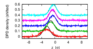
As already noted in the main text (Section III.1), the DPD particles represent the total density of the fluid, including neutral solvent and small ions. To illustrate this, we consider an equilibrium system (stationary and ) in an electrostatic potential . Eq. (1) ensures that the ions are Boltzmann distributed, . Combining this with Eq. (3), one obtains the equilibrium relation . Since our DPD particles have no conservative interactions, they have ideal gas statistics and the local pressure (excluding electrostatics) satisfies . Hence the ”neutral solvent density” fulfills , i.e., is constant everywhere as one would expect. The shape of the DPD profile therefore follows that of the total ion profile:
| (22) |
The distribution defines an effective potential acting on DPD particles, , from which one can derive an effective force . The latter can be related to the total force acting on all ions, , via
| (23) |
This equation is consistent with the requirement that the total force acting on the DPD fluid must match the total force acting on all pseudo ions (Section B.3).
Ideally, the coupling scheme between pseudo ions and DPD particles should ensure both an accurate distribution coupling (Eq. (22)) and an accurate force coupling (Eq. (23)). Unfortunately, this is not feasible for finite grids. Only one type of coupling can be implemented exactly. Since momentum conservation is crucial in hydrodynamics, the Condiff-DPD algorithm was constructed to ensure exact force coupling. This automatically leads to discretization artefacts in the distribution of DPD particles.
To illustrate and investigate these effects, we study a bulk system of size exposed to a quadratic external electrostatic potential . The ions are then localized in the potential well, and the DPD profile reflects the peak of the ion distribution. We vary the grid spacing between and . The resulting profiles for charge assignment order cao3 are shown in Fig. 10. At larger grid spacings, the DPD profile does not fully follow the ion profile. Reasonable agreement is obtained for , which is the standard grid spacing used in the present work.

The artifacts in the DPD profiles are most pronounced close to impenetrable walls, where high surface charges may generate large charge gradients. We find that this leads to an excess of DPD particles close to the surfaces. Fig. 11 compares ion profiles and shifted DPD density profiles in a slit channel of width containing counterions only for different surface charge densities . At low , the profiles match well (Fig. 11a). At higher , a disproportionately high number of DPD particles accumulates at the walls. For extreme surface charges , the DPD particles may even withdraw entirely from the bulk of the slab.
This problem can easily be remedied either by using smaller grid spacings or by introducing repulsive interaction between DPD particles, i.e., making the fluid less compressible. In the applications presented in this paper, however, this was not necessary because the deviations of the ideal DPD profile shapes were small. The DPD density profiles are not the focus of interest in this work. We only need to ensure that the DPD fluid reproduces the correct fluid dynamics. Thus the algorithm must guarantee a faithful force transmission between pseudo-ions and DPD particles, and the shear viscosity of the fluid should be roughly constant. This is still the case, even if the DPD density varies slightly.
Appendix D Tunable slip algorithm applied to electrolytes

The tunable slip algorithm by Smiatek et al. [25] is designed to implement hydrodynamic boundary conditions with arbitrary slip lengths in DPD simulations. This is done by introducing a thin viscous layer covering the walls, which is implemented in terms of a locally varying friction function. The slip length is controlled by the friction between the fluid and the wall, more precisely by the shape, the amplitude, and the range of the friction function. For example, if one assumes that the fluid density is constant up to a hard boundary at and if one chooses a linearly varying friction function , a good analytical estimate of the slip length is provided by the formula [25]
| (24) |
with and . For neutral fluids, this equation is reasonably accurate at high , but becomes problematic at low . Corrections based on numerical simulations have recently been proposed by Zhou et al. [58].
ln our model electrolyte fluids, the density of the DPD fluid increases close to charged walls (see Appendix C.2). Therefore is no longer constant, and Eq. (24) no longer applies. Nevertheless, we find that it can still be used after a simple heuristic modification: It suffices to replace the density in the dimensionless factor by an effective density
| (25) |
In practice, we fit the function by a second order polynomial before performing the integration. Furthermore, we allow for a uniform offset in Eq. (24), which provides us with a single fit parameter . With these adjustments, Eq. (24) is found to fit the simulation data for the slip length over a wide range of (Fig. 12a). Here we have simulated an electrolyte fluid with Debye screening length close to a homogeneous charged surface with surface charge density . The slip length data are obtained by a joint analysis of Poiseuille and Couette flows following Ref. [25]. The density renormalization leads to a slight decrease of for given friction amplitude (Fig. 12b)).
References
- [1] C. Holm and K. Kremer, Advanced computer simulation approaches for soft matter sciences I, Vol. 1 (Springer, 2005)
- [2] G. W. Slater, C. Holm, M. V. Chubynsky, H. W. de Haan, A. Dubé, K. Grass, O. A. Hickey, C. Kingsburry, D. Sean, T. N. Shendruk, et al., Electrophoresis 30, 792 (2009)
- [3] K. Kremer, Macromolecular Chemistry and Physics 204, 257 (2003)
- [4] F. Müller-Plathe, ChemPhysChem 3, 754 (2002)
- [5] S. O. Nielsen, C. F. Lopez, G. Srinivas, and M. L. Klein, Journal of Physics: Condensed Matter 16, R481 (2004)
- [6] M. Kröger, Physics Reports 390, 453 (2004)
- [7] M. Deserno and C. Holm, Journal of Chemical Physics 109, 7678 (1998)
- [8] R. Groot, Journal of Chemical Physics 118, 11265 (2003)
- [9] M. González-Melchor, E. Mayoral, M. E. Velázquez, and J. Alejandre, Journal of Chemical Physics 125, 224107 (2006)
- [10] G. A. Cisneros, M. Karttunen, P. Ren, and C. Sagui, Chemical Reviews 114, 779 (2014)
- [11] R. W. Hockney and J. W. Eastwood, Computer simulation using particles (Taylor & Francis, 1988)
- [12] J. Smiatek and F. Schmid, in Advances in Microfluidics, edited by R. T. Kelly (InTech Open Access Publisher, Rijeka, 2012) pp. 97–126
- [13] K. Kim, Y. Nakayama, and R. Yamamoto, Physical Review Letters 96, 208302 (2006)
- [14] F. Capuani, I. Pagonabarraga, and D. Frenkel, Journal of Chemical Physics 121, 973 (2004)
- [15] J. P. Hernández-Ortiz, J. J. de Pablo, and M. D. Graham, Physical Review Letters 98, 140602 (2007)
- [16] S. Fischer, A. Naji, and R. R. Netz, Physical Review Letters 101, 176103 (2008)
- [17] D. Duong-Hong, J. Han, J.-S. Wang, N. G. Hadjiconstantinou, Y. Z. Chen, and G.-R. Liu, Electrophoresis 29, 4880 (2008)
- [18] O. A. Hickey, C. Holm, J. L. Harden, and G. W. Slater, Physical Review Letters 105, 148301 (2010)
- [19] O. A. Hickey, T. N. Shendruk, J. L. Harden, and G. W. Slater, Physical Review Letters 109, 098302 (2012)
- [20] M. Joulaian, A. Pishevar, S. Khajepor, F. Schimd, and Y. Afshar, Computer Physics Communications 183, 2405 (2012)
- [21] R. Kekre, J. E. Butler, and A. J. C. Ladd, Physical Review E 82, 050803(R) (2010)
- [22] J. Zhou, R. Schmitz, B. Dünweg, and F. Schmid, The Journal of Chemical Physics 139, 464112 (2013)
- [23] P. Hoogerbrugge and V. Koelman, Europhys. Lett 19, 155 (1992)
- [24] P. Español and P. Warren, EPL (Europhysics Letters) 30, 191 (1995)
- [25] J. Smiatek, M. P. Allen, and F. Schmid, The European Physical Journal E: Soft Matter and Biological Physics 26, 115 (2008)
- [26] S. Meinhardt, J. Smiatek, R. Eichhorn, and F. Schmid, Physical Review Letters 108, 214504 (2012)
- [27] J. Zhou, A. V. Belyaev, F. Schmid, and O. I. Vinogradova, Journal of Chemical Physics 136, 194706 (2012)
- [28] P. Szymczak and A. Ladd, Physical Review E 68, 036704 (2003)
- [29] J. Honerkamp, Stochastic Dynamical Systems: Concepts, Numerical Methods, Data Analysis (Wiley, 1993)
- [30] J. D. Weeks, D. Chandler, and H. C. Andersen, Journal of Chemical Physics 54, 5237 (1971)
- [31] J. Smiatek, M. Sega, C. Holm, U. D. Schiller, and F. Schmid, The Journal of Chemical Physics 130, 244702 (2009)
- [32] H.-J. Limbach, A. Arnold, B. A. Mann, and C. Holm, Computer Physics Communications 174, 704 (2006)
- [33] http://espressomd.org
- [34] A. Arnold, J. de Joannis, and C. Holm, Journal of Chemical Physics 117, 2496 (2002)
- [35] C. Marsh, G. Backx, and M. Ernst, Physical Review E 56, 1676 (1997)
- [36] I. Pagonabarraga, M. H. J. Hagen, and D. Frenkel, Europhysics Letters 42, 377 (1998)
- [37] G. Besold, I. Vattulainen, M. Karttunen, and J. M. Polson, Physical Review E 62, R7611 (2000)
- [38] T. Shardlow, SIAM Journal on Scientific computing 24, 1267 (2003)
- [39] M. Serrano, G. de Fabritiis, P. Espanol, and P. V. Coveney, Math. Comput. Simul. 72, 190 (2006)
- [40] G. de Fabritiis, M. Serrano, P. Espanol, and P. V. Coveney, Physica A 361, 429 (2006)
- [41] R. Probstein, Physicochemical Hydrodynamics: An Introduction (Wiley, 2005)
- [42] J. Lyklema, H. P. van Leeuwen, M. Vliet, and A.-M. Cazabat, Fundamentals of interface and colloid science, Vol. 5 (Academic Press, 2005)
- [43] J. Smiatek and F. Schmid, The Journal of Physical Chemistry B 114, 6266 (2010)
- [44] R. J. Hunter, Foundations of colloid science (POD), 2nd ed. (Oxford University press, 2000)
- [45] C. I. Bouzigues, P. Tabeling, and L. Bocquet, Physical Review Letters 101, 114503 (2008)
- [46] J. Ou and J. P. Rothstein, Physics of Fluids 17, 103606 (2005)
- [47] M. Z. Bazant and O. I. Vinogradova, Journal of Fluid Mechanics 613, 125 (2008)
- [48] C. Schönecker, T. Baier, and S. Hardt, Journal of Fluid Mechanics 740, 168 (2014)
- [49] A. V. Belyaev and O. I. Vinogradova, Physical Review Letters 107, 98301 (2011)
- [50] E. S. Asmolov, J. Zhou, F. Schmid, and O. I. Vinogradova, Physical Review E 88, 023004 (2013)
- [51] H. Zhao, Physical Review E 81, 066314 (2010)
- [52] This holds in the Poisson-Boltzmann (the mean field) regime. If charge fluctuations are important, the number of pseudo-particle should match the number of real ions.
- [53] P. D. Grossman and J. C. Colburn, Capillary Electrophoresis, Theory and Practice: Free Solution Capillary Electrophoresis (Academic Press, San Diego, 1992)
- [54] J. Zhou and F. Schmid, J. Phys.: Cond. Matter 24, 464112 (2012)
- [55] I. C. Yeh and M. L. Berkowitz, The Journal of Chemical Physics 111, 3155 (1999)
- [56] H. G. Petersen, Journal of Chemical Physics 103, 3668 (1995)
- [57] M. Deserno and C. Holm, Journal of Chemical Physics 109, 7694 (1998)
- [58] J. Zhou, E. S. Asmolov, F. Schmid, and O. I. Vinogradova, Journal of Chemical Physics 139, 174708 (2013)