Robust Adaptive Quantum Phase Estimation
Abstract
Quantum parameter estimation is central to many fields such as quantum computation, communications and metrology. Optimal estimation theory has been instrumental in achieving the best accuracy in quantum parameter estimation, which is possible when we have very precise knowledge of and control over the model. However, uncertainties in key parameters underlying the system are unavoidable and may impact the quality of the estimate. We show here how quantum optical phase estimation of a squeezed state of light exhibits improvement when using a robust fixed-interval smoother designed with uncertainties explicitly introduced in parameters underlying the phase noise.
Keywords: quantum phase estimation, robust estimator, optimal estimator, smoothing, squeezed state.
1 Introduction
Quantum parameter estimation [1] is the problem of estimating a classical variable of a quantum system. It plays a key role in quantum computation [2], quantum communications [3, 4], quantum key distribution [5], metrology [6] and gravitational wave interferometry [7], etc. A common and technologically relevant example is estimating an optical phase in a quantum system. Optimal estimation theory has earlier been considered in devising and improving quantum parameter estimation techniques. Systematic approaches to optimal estimation yield estimates with the lowest mean-square estimation error. This has helped achieve better estimation accuracies than otherwise obtained previously [8, 9].
Nonetheless, the optimality of the estimation process relies on precise knowledge of the system model. However, this is usually unrealistic due to inevitable modelling errors. In many cases, it is impossible to precisely measure and determine values of relevant model parameters in an experiment. This is detrimental in problems of quantum estimation because any uncertainty in our knowledge of the parameters in the system model may result in considerable degradation in the estimation accuracy. It is, therefore, desired to make the estimation process robust to uncertainties in the underlying model parameters [10, 11].
It is important in many practical engineering problems to ensure that the critical measures of the system performance do not deviate beyond certain thresholds. Such thresholds mark the point beyond which the system has a high risk of breaking down or becoming unusable. In quantum estimation problems, performance is typically determined by the error in the estimation process in the presence of uncertainty in the system. An optimal estimator is optimized by minimizing a cost function to yield the least mean-square estimation error for exact model parameters. When the model parameters are not the same as the true system parameters, i.e. when there is uncertainty in one or more of the model parameters, the true estimation error may be worse than the predicted optimal value. In a worst-case situation with large uncertainties, this increase in the size of the estimation errors could be significant. A robust estimator, on the other hand, can be designed by optimizing the worst case of a cost function for an uncertain system model. This allows the robust estimator to yield lower estimation errors than the optimal estimator in the worst-case scenario. For example, in gravitational wave detection, large estimation errors may mask a gravitational-wave event or imitate an event. Such a false event may be avoided using a robust estimator, which has a sufficient guaranteed worst-case precision.
In this paper, we aim to design a robust estimator for quantum phase estimation that provides guaranteed worst-case performance. Robust quantum parameter estimation was previously considered in Ref. [12] for magnetometry. That paper employed heuristic feedback mechanism to achieve robustness. By contrast, we consider a more systematic approach to robust estimation in a state-space setting with explicitly modelled uncertainty. Among other related works, Ref. [13] proposed a robust quantum observer for uncertain linear quantum systems and Ref. [14] considered robustness in the context of coherent feedback. However, for linear quantum systems, much of the rich classical estimation theory may be applied. To our knowledge, the potential application of classical robust estimation theory has not yet been explored in improving quantum estimation techniques.
Quantum phase estimation has been area of active research recently [15, 16, 17, 18, 19, 20, 21, 22]. Adaptive quantum phase estimation of the continuously varying phase of a coherent state of light using smoothing was demonstrated in Ref. [8]. Fixed-interval smoothing uses both past and future measurements in a fixed time-interval to yield a more accurate estimate than obtained using only past measurements [23, 24, 25, 26, 27, 28, 29, 30]. Using a robust fixed-interval smoother [31], the estimation process for the adaptive experiment can be improved in the presence of uncertainty in the underlying phase noise subject to an Ornstein-Uhlenbeck (OU) noise [32]. While a coherent state has the same uncertainty in both (amplitude and phase) quadratures, a squeezed state has reduced fluctuations in one of the two quadratures at the expense of increased fluctuations in the other. Using a squeezed state of light provides quantum enhancement in adaptive phase tracking [9]. Here, we illustrate the guaranteed worst-case performance of the robust estimator for such a squeezed state [33]. We model the phase to be estimated as an OU process to begin with in our paper because Refs. [8] and [9] consider such a noise mechanism. The idea is to demonstrate the improvement provided by our robust estimator over the optimal estimator used in the noise setting of Ref. [9]. Such a stochastically varying phase resembles a continuous-time random walk with a tendency to return to the mean phase of zero, a kind of noisy relaxation process that occurs in many physical situations, and is more relevant for applications such as physical metrology and communication than a time-invariant (but initially unknown) phase [9].
The robust fixed-interval smoothing scheme can as well be applied to estimate a phase, modelled as a resonant noise process with uncertainty in its parameters [34]. A related robust filtering problem for coherent state was considered by the authors for OU process in Ref. [35] and for resonant process in Ref. [36]. Here, we build on the results in the conference paper [34] to provide interesting insights about the guaranteed worst-case performance of the robust estimator. Moreover, we show that the performance improvement of the robust estimator relative to the optimal estimator grows as the noise process becomes more resonant. We also show here that the worst-case performance of our robust estimator relative to the optimal estimator is better for realistic lossy squeezed beams than that for ideal pure squeezed beams at the optimal degrees of squeezing. In addition, we illustrate that our robust estimator exhibits an optimal photon number for which its relative performance is the best with respect to the optimal estimator.
2 Optimal Estimator
The optimal estimator in Ref. [9] involves an offline optimal smoother, in addition to a Kalman filter in the feedback loop. The feedback Kalman filter is a causal filter. However, the smoother is acausal, since it is, in principle, a combination of a forward-time Kalman filter and a backward-time Kalman filter, the estimates of which are combined to yield the optimal smoothed estimate [37]. While the forward Kalman filter is essentially the feedback filter itself and uses only past measurements, the backward filter yields its estimate based on future measurements with respect to the time of the desired smoothed estimate within the chosen fixed time-interval . A smoother, therefore, cannot be used to produce real-time estimates, and is usually used for offline data processing or with a delay with respect to the estimation time to yield more accurate estimates than obtained using the feedback Kalman filter alone [8, 9].
2.1 System Model
We need to define our system in terms of the process and measurement models in a state-space setting.
The process model is the OU noise process that modulates the phase , to be estimated, of the continuous optical phase-squeezed beam [9]:
| (1) |
where is the correlation time of , is the phase variation magnitude and is a zero-mean white Gaussian noise with unity amplitude.
The phase-modulated beam is measured by homodyne detection using a local oscillator, the phase of which is adapted with the filtered estimate using feedback, thereby yielding a normalized homodyne output photocurrent [9]:
| (2) | |||||
| (3) |
where is the amplitude of the input phase-squeezed beam, and is a Wiener process arising from squeezed vacuum fluctuations. The parameter is determined by the degree of squeezing () and anti-squeezing () and by (see later). We use the measurement appropriately scaled as our measurement model [33]:
| (4) |
where is also a zero-mean white Gaussian noise with unity amplitude.
Here, , , , where denotes the expectation value and is the delta function. Since and are of unity amplitude, both and are unity.
2.2 Forward Filter
For the process and measurement models given by (1) and (4) respectively, the standard steady-state Kalman filter is constructed by solving a continuous-time algebraic Riccati equation as in A.
The steady-state Riccati equation to be solved for the forward Kalman filter is:
| (5) |
where is the forward filter error-covariance. The stabilising solution of the above equation is:
| (6) |
The forward filter equation is:
| (7) |
where is the forward Kalman gain.
2.3 Backward Filter
The steady-state backward Kalman filter is constructed similarly as in A.
The steady-state Riccati equation to be solved for the backward Kalman filter is:
| (8) |
where is the backward filter error-covariance. The stabilising solution of the above equation is:
| (9) |
The backward filter equation is:
| (10) |
where is the backward Kalman gain.
2.4 Smoother Error
3 Robust Estimator
Here, we build a robust fixed-interval smoother, corresponding to the optimal smoother above, using the technique from Ref. [31] as outlined in B.
3.1 Uncertain Model
The uncertainty is introduced in the parameter as follows: where determines the level of uncertainty in the model, and is an uncertain parameter satisfying:
| (13) |
which is of the form (58). Also, the noises and are assumed to satisfy the following bound for a suitable constant :
| (14) |
which is of the form (59) with . Moreover, no a-priori information exists about the initial condition of the state, and therefore, we choose in (60).
Then, the corresponding uncertain system model takes the form:
| (15) |
which is of the form (57). Here and . Also, here in (57), since there is no known input in our case. Moreover, here and in (57).
Remark.
As outlined in B, the robust fixed-interval smoother takes the form of an ellipse of possible states and the centre of this ellipse is the robust smoother estimate. This robust smoother estimate will be given in terms of two quantities referred to as the forward filter state and the backward filter state, which are defined in the following sections.
3.2 Forward Filter
The steady-state forward Riccati equation used in the robust smoother, as obtained from (73), is:
| (16) |
The stabilising solution of the above equation for is:
| (17) |
Next, the equation (75), that forms part of the robust smoother, for our case yields:
| (18) |
We then define the quantity, , which is referred to as the forward filter state.
Thus, the forward robust filter equation is
| (19) |
where .
For , (19) reduces to (7), i.e. the robust forward filter is simply the forward Kalman filter for zero uncertainty level.
Remark.
The quantity is actually the centre of an ellipse defined by the solution to a robust filtering problem; see Theorem 3.1 in Ref. [31]. However, this property will not be used here.
3.3 Backward Filter
The steady-state backward Riccati equation for the robust smoother, as obtained from (74), is:
| (20) |
The stabilising solution of the above equation for is:
| (21) |
Next, the equation (77), that forms part of the robust smoother, in reverse-time yields:
| (22) |
We then define the quantity, , which is referred to as the backward filter state.
Thus, the backward robust filter equation is
| (23) |
where again .
For , (23) reduces to (10), i.e. the robust backward filter is the same as the backward Kalman filter for zero uncertainty level.
Remark.
The quantity is actually the centre of an ellipse defined by the solution to a robust retrodiction (i.e. backward-time filtering) problem; this is similar to the robust (forward) filtering problem considered in Theorem 3.1 in Ref. [31]. However, this property will not be used here.
3.4 Robust Smoother
The robust smoother estimate is the centre of the ellipse defined in (78) and is given in terms of and according to the following formula:
| (24) |
4 Comparison of Estimators
We shall now compare the mean-square estimation errors of the optimal and robust estimators for the uncertain system.
4.1 Error Analysis
Given the forward and backward filter dynamics for the uncertain system, the mean-square errors for are computed using the following method employing a Lyapunov equation. Here, we shall illustrate the method for the optimal estimator only. The errors for the robust estimator may be calculated similarly.
4.1.1 Forward Filter
The uncertain system, given by
| (25) |
augmented with the forward-time Kalman filter (7) may be represented by the state-space model:
| (26) |
where , .
Thus, we have
The steady-state state covariance matrix is obtained by solving the Lyapunov equation:
| (27) |
where is the symmetric matrix
| (28) |
Here, , , and .
The estimation error can be written as:
| (29) |
which is mean zero since all of the quantities determining are mean zero. The error covariance is then given as:
| (30) |
4.1.2 Backward Filter
When our uncertain model (25), (4), which is driven by Gaussian white noise, has reached steady state, the output process will be a stationary Gaussian random process, which is described purely by its auto-correlation function. If we consider this output process in reverse time, this will also be a stationary random process with the same auto-correlation function. This follows from the definition of the auto-correlation function. Hence, the statistics of the reversed time output process are the same as the statistics of the forward time output process. Thus, the reversed time output process can be regarded as being generated by the same (and not time reversed) process (25) that generated the forward time process [32].
The error covariance for the backward filter is then:
| (32) |
where .
4.1.3 Smoother Error
The forward and backward estimates are not independent in general and will have a cross-correlation term as follows [32]:
| (33) |
where and [27].
The overall smoother error for the optimal estimator is (see Eq. (25) in Ref. [32]):
| (34) |
4.2 Comparison of the Errors
The error-covariances of the robust smoother and the optimal smoother for the uncertain system may be computed using the above technique by solving a Lyapunov equation, as a function of . Here, we choose the value of and the other parameters as in Ref. [9], viz. , rad/s, rad/s, and . Due to the implicit dependence of and ((3) and (30)), we compute the smoothed mean-square error (34) and (35) by running several iterations until is obtained with an accuracy of decimal places in each case. Fig. 1 shows a comparison for , which corresponds to uncertainty in . At , where the nominal parameters for the model exactly match those of the system, the optimal smoother performs better than the robust smoother. This is to be expected because the smoother has been optimised for those parameters. However, the robust smoother error is lower than that of the optimal smoother as approaches . We define as the worst-case estimation error for each value of , i.e. . So, if our system is not allowed to exceed an error threshold of say for this level of uncertainty in , our robust estimator guarantees that the error is below this threshold, whereas the optimal estimator breaches it in the worst case.

Fig. 2 shows the comparison of the worst-case performance of the optimal and the robust estimators for the uncertain system for . Clearly, the robust estimator provides with better worst-case performance than the optimal estimator for all levels of uncertainty in . Also, the worst-case robust estimator error is below a desired threshold of say for up to a higher level of uncertainty as compared to the optimal estimator. This is exactly the power of robust design techniques.

5 Resonant Noise Process
We now consider a second-order resonant noise process, typically produced by a piezo-electric transducer (PZT) driven by an input white noise. Such a resonant process is more complicated than the simplistic OU noise process considered before and better resembles the kind of noises that in practice corrupt the signal. The simplified transfer function of a typical PZT is (see the supplementary material of Ref. [38]) as follows:
| (36) |
where is the gain, is the damping factor, is the resonant frequency (rad/s), is a zero-mean white Gaussian noise with unity amplitude and is the PZT output that modulates the phase to be estimated.
5.1 System Model (Exact)
Eq. (37) constitutes our process model, whereas the measurement remains the same as (4). Thus, our measurement equation is
| (38) |
where .
In this paper, we choose parameter values which are particularly suited to the illustration of our key robustness results and yet represent a possible physical situation, viz. , and rad/s and .
5.2 Uncertain Model
We introduce uncertainty in as follows:
| (39) |
where uncertainty is introduced in the resonant frequency through . Although uncertainty in would affect both entries in the second row of the above matrix, the most significant effect will be in the term. Indeed, since we have a resonant system and , the uncertainty in term can be neglected for simplicity and to give a less conservative estimator.
Here, is an uncertain parameter satisfying which implies . Moreover, determines the level of uncertainty. From (57), the uncertain model here is:
| (40) |
where .
5.3 Comparison of the Estimators
The optimal and robust estimators can be constructed for the resonant noise case using the same method employed in the OU noise case before. The mean-square errors in estimation of may be computed using the error-analysis technique discussed before for both the optimal smoother and robust fixed-interval smoother as a function of the uncertain parameter . Note that , in (6),(7), , in (9),(10), in (17), and in (21) are matrices, and not scalars, in this resonant noise case. Thus, the expressions in (30), (32) and (33) yield matrices, and not scalars, in this resonant noise case for both the optimal and robust smoothers, but the values that we use to compute the effective smoother error (34) and (35) here are the entries in these matrices, since we are interested in the estimation errors in and not from in (40). These values can be used to generate a plot of the errors versus for a given value of to compare the performance of the robust smoother and the optimal smoother for the uncertain system. Here, we used the nominal parameter values, and and to have an optimal squeezing level, for which the estimation error is the minimum for the exact model [9]. Again, due to the implicit dependence of and , we compute the smoothed mean-square error (34) and (35) by running several iterations until is obtained with an accuracy of decimal places in each case.
It is also insightful to include in the graph the coherent state limit (CSL), which is the minimum theoretical error reachable with a coherent beam [9]. The CSL value is obtained by designing a different optimal smoother for each value of the uncertain parameter in (40) (note , and for coherent beam), and is given by from (11). We as well include the standard quantum limit (SQL), which is the minimum phase estimation error that can be obtained with coherent beam using perfect heterodyne technique. The method to compute the SQL for our resonant noise model is given in C. The SQL value is obtained for our plots for each value of the uncertain parameter in the process model in (40), with the measurement model in (83). Fig. 3 shows the plot for .

One can see that the optimal smoother behaves better than the robust smoother when , as expected. However, in the worst-case scenario, i.e. as approaches , the performance of the robust smoother is superior to that of the optimal smoother. Nonetheless, we trade off the best-case performance in achieving it. It is also of relevance that the robust estimator beats the SQL over a larger part of the uncertainty window than the optimal estimator, although this is not the case with respect to the CSL for this value of .
Fig. 4 depicts the worst-case performance of the estimators for . Clearly, the robust estimator outperforms the optimal estimator in the worst-case for all levels of . Also shown in the plot are the SQL and the CSL. If the SQL or the CSL is considered as the allowed threshold for the estimation error, our robust estimator provides guaranteed worst-case performance below this threshold for up to a larger uncertainty level when compared to the optimal estimator.

Moreover, the improvement with the robust smoother over the optimal smoother is better with the resonant noise process considered here as compared to that with OU noise process considered before. For example, while the worst-case improvement for uncertainty in the OU noise case was dB, that in this resonant noise case is dB. Indeed, OU noise is the output of a non-resonant low-pass filter (LPF), driven by white noise. Any uncertainty in the corner frequency of the LPF, represented by here, would not change the magnitude of the phase noise as much as an equivalent amount of uncertainty in the resonant frequency for the resonant noise model. In fact, the relative performance of our robust estimator grows as the noise process becomes more resonant. This is shown in Fig. 5, which plots the worst-case errors of the optimal and robust smoothers as a function of the damping factor , that determines the degree of resonance; i.e. the lower damping factor, the more resonant the process is. Here, at each value of , the squeezing level has been optimized to yield the minimum error for the exact model.

Fig. 6 shows a plot of the worst-case errors of the smoothers as functions of the squeezing level. Here, we have plotted the errors for pure lossless squeezed beams (overall loss ) and practical impure lossy squeezed beams with (see the supplementary material for Ref. [9]), and a fixed uncertainty level of . Clearly, our robust estimator not only beats the CSL over a wider range of squeezing levels (for both pure and impure squeezing cases), but also can sustain higher levels of squeezing than the optimal estimator can, before the errors rapidly increase due to excessive anti-squeezing noise. Moreover, our estimator is more robust relative to the optimal estimator for practical squeezed beams than for ideal pure squeezed beams. This is due to the larger worst-case performance benefit obtained in the practical case than in the ideal case at the optimal squeezing levels. While the robust estimation worst-case error is dB lower than the optimal estimation worst-case error at the optimal squeezing level of dB for the lossless case, the robust estimation worst-case performance is dB better than the optimal estimation worst-case performance at the optimal squeezing level of dB for the lossy case. That is, our estimator, which was designed to be robust to uncertainty in the resonant frequency , is also robust, relative to the optimal estimator, against the overall loss , arising from imperfect detectors, the optical parametric oscillator (OPO) and modulators.

Finally, we plot the worst-case errors of the estimators against the photon flux in Fig. 7. Here, at each value of , the squeezing level has been optimized to yield the least worst-case robust estimation error. One can choose to optimize the squeezing level on a different basis as well. Interestingly, not only do the two errors scale differently with the photon flux, but also note there exists an optimum photon flux, and therefore an optimum photon number, for which the robust estimator provides the best worst-case performance compared to the optimal estimator. This is quite significant, given how important the achievable precision for available finite quantum resources is in practice.

6 Conclusion
This work considered robust quantum phase estimation with explicitly modelled uncertainty introduced in the underlying system in a systematic state-space setting within the modern control theory paradigm. In particular, we constructed a robust fixed-interval smoother for continuous phase estimation of a squeezed state of light with uncertainty considered in the phase noise. We illustrated that our robust estimator provides guaranteed worst-case performance as desired. We showed that the worst-case performance of our robust estimator with respect to the optimal estimator improves with greater resonance in the phase noise. Moreover, we found that robustness is more useful for practical lossy squeezed beams, when compared to pure squeezed beams, ideally limited by Heisenberg’s uncertainty principle. In addition, we saw that there is an optimal photon number for which the performance of the robust estimator relative to the optimal estimator is the best. These results demonstrate the significant impact that the rich theory of classical robust estimation can have on improving quantum parameter estimation. They can pave the way for tackling practical challenges owing to unavoidable parametric uncertainties facing quantum parameter estimation.
Acknowledgments
This work was supported by the Australian Research Council. The first author would like to thank Dr. Hongbin Song, Dr. Obaid Ur Rehman, Trevor Wheatley, Prof. Howard Wiseman and Dr. Dominic Berry for useful discussion and feedback related to this work.
Appendix A Kalman Filtering and Optimal Smoothing Theory
We first outline here the continuous-time formulation of the Kalman filter, called the Kalman-Bucy filter. Then we outline the optimal two-filter smoothing theory, as discussed in Ref. [37], but using our notation.
A.1 Kalman Filter
The process and measurement models are assumed to be of the form:
| (41) |
where
| (42) |
Here, the noises and are assumed to be vector white-noise processes with zero cross-correlation. Also, is the state of the process to be estimated and is the measurement output. Note that the matrices , , and may be time-varying.
Then, the error-covariance matrix of the Kalman filter is the stabilizing solution of the following matrix differential Riccati equation:
| (43) |
where is the initial error-covariance.
In the steady-state case, the Riccati equation to be solved to construct the Kalman filter is the following algebraic Riccati equation:
| (44) |
Note that the above Riccati equation is quadratic in .
The gain of the Kalman filter, called the Kalman gain, is then given as:
| (45) |
The continuous Kalman filter equation is given as:
| (46) |
where is the desired estimate of the state and is the initial state estimate.
A.2 Optimal Smoother
The two-filter smoother, as its name suggests, consists of two different filters, one forward-time, and one backward-time, whose estimates are combined to yield a final smoothed estimate [37].
Let us assume that data is available over a fixed time-interval , and we desire an optimal smoothed estimate at a point . The forward-time variables will be denoted with subscripts, such as , and backward-time variables with subscripts, such as . The process and measurement models for the forward-time filter would be:
| (47) |
where (42) holds. The time variable in this case is , running forward in time.
Then, the steady-state Riccati equation to be solved for the forward filter is:
| (48) |
Also the filter equation is given as:
| (49) |
Here, the forward Kalman gain is:
| (50) |
For the backward filter, it is convenient to define a new running time variable that proceeds backward in time. Note that corresponds to . The backward process model is then obtained by replacing the time derivative in the above process model with :
| (51) |
The Riccati and filter equations may then be obtained by replacing and in the corresponding equations for the forward filter with and , respectively.
The backward filter steady-state Riccati equation is:
| (52) |
The backward filter equation is:
| (53) |
Here, the backward Kalman gain is:
| (54) |
The smoothing error-covariance is then computed as:
| (55) |
The equation for the smoothed estimate is then:
| (56) |
Appendix B Robust Fixed-Interval Smoothing Theory
We outline here the robust fixed-interval smoothing theory from Ref. [31], but using our notation. Consider an uncertain system described by the state equations
| (57) |
where is the state, is the measured output, is a known input, and are noises. and are matrices. Furthermore, and are uncertainty matrices satisfying
| (58) |
for all , where and are weighting matrices. Then, for a given finite time-interval and a given suitable constant , we require the noises to satisfy the inequality
| (59) |
Let be a given matrix, be a given real vector, be a given suitable constant. Then, we assume the initial conditions satisfy the inequality
| (60) |
This uncertain system is a special case of the uncertain system considered in Eq. (3.19) of Ref. [31] of the following form:
| (61) |
where the output defines the structure of the uncertainty in the uncertain system model, and the quantities and are given by
| (62) |
Let us consider weighting matrices and . Then, using (62), we have:
| (63) |
Also, for a given constant , the following holds, since :
| (64) |
This implies
| (65) |
Similarly, since , we have
| (66) |
This implies
| (67) |
Now, we let
| (69) |
Since can be chosen to be arbitrarily small, then and will be arbitrarily close to and , respectively.
We now let
| (71) |
Then, it follows from (60), (70) and (71) that the following integral quadratic constraint (IQC) is satisfied by the uncertainty in the system (61):
| (72) |
which corresponds to Eq. (3.20) in Ref. [31].
As mentioned above, and can be chosen to be arbitrarily close to and , respectively. For simplicity, in the sequel, we will take and .
A steady-state solution to the robust fixed-interval smoothing problem for this uncertain system involves the algebraic Riccati equations:
| (73) | ||||
| (74) |
It will also include a solution to the differential equations:
| (75) |
for and
| (76) |
for . Here, is a fixed measured output of the uncertain system (61), defined on the time interval , and is a fixed measured input to the uncertain system defined on the same time interval.
Note that the form of (76) we are interested in is with respect to the running time variable that proceeds backward in time:
| (77) |
for .
Theorem 1
Clearly, the set of all possible states in (78) is an ellipsoid, and the best estimate of the state is chosen as the centre of the ellipsoid.
Remark.
In the above, and have been chosen to be arbitrarily close to and , respectively, which corresponds to small . In the limit , in (71), and therefore in (72), approaches infinity. However, in practice there will be a trade-off between how close and are to and , respectively, and how large is . The proposed theory is perfectly valid for finite values of in the IQC of (72), and it is never intended that the limit as approaches infinity should be considered.
Increasing the value of increases the diameter of the state estimation ellipse. However, the centre of the ellipse and hence the robust estimate is independent of . Hence, in examples such as the one considered in this paper, in which we are only interested in the robust estimator (whose performance is validated via other means) and not the estimation ellipse, it would not be a problem if the value of chosen is very large (but finite).
Appendix C Standard Quantum Limit (SQL) for Resonant Noise
The standard quantum limit is set by the minimum error in phase estimation that can be obtained using a perfect heterodyne scheme with a coherent beam [32, 36]. We use the fact that the heterodyne scheme of measurement is, in principle, equivalent to, and incurs the same noise penalty as the dual-homodyne scheme [8], such as in the schematic depicted in Fig. 8. A coherent signal at the input is phase-modulated using an electro-optic modulator (EOM) that is driven by the resonant noise source. The modulated signal is then split using a beamsplitter into two arms each with a homodyne detector (HD1 and HD2, respectively, with the local oscillator phase of HD1 out of phase with that of HD2). The ratio of the output signals of the two arms goes to an arctan block. The output of the arctan block is fed to an optimal Kalman filter, that yields the phase estimate with the minimum estimation error.
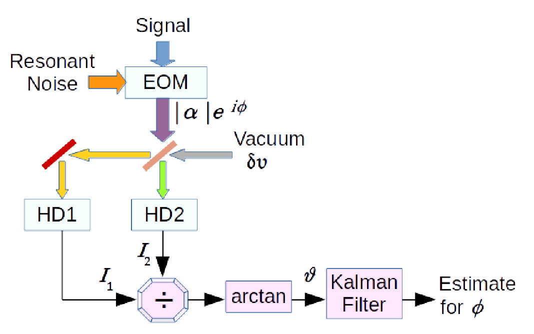
The output signals of the two arms are [32, 36]:
| (80) |
where and are measurement noises of the two homodyne detectors, respectively, and and are the noises arising from the vacuum entering the empty port of the input beamsplitter corresponding to the two arms, respectively. All these noises are assumed to be zero-mean white Gaussian noises.
Assuming the input noises are small, a Taylor series expansion up to first-order terms of the right-hand side yields [32, 36]:
| (82) |
References
References
- [1] Wiseman H M and Milburn G J 2010 Quantum Measurement and Control (Cambridge University Press)
- [2] Hofheinz M, Wang H, Ansmann M, Bialczak R C, Lucero E, Neeley M, O’Connell A D, Sank D, Wenner J, Martinis J M and Cleland A N 2009 Nature (London) 459 546–549
- [3] Slavik R, Parmigiani F, Kakande J, Lundstrom C, Sjodin M, Andrekson P A, Weerasuriya R, Sygletos S, Ellis A D, Gruner-Nielsen L, Jakobsen D, Herstrom S, Phelan R, O’Gorman J, Bogris A, Syvridis D, Dasgupta S, Petropoulos P and Richardson D J 2010 Nature Photonics 4 690–695
- [4] Chen J, Habif J L, Dutton Z, Lazarus R and Guha S 2012 Nature Photonics 6 374
- [5] Inoue K, Waks E and Yamamoto Y 2002 Physical Review Letters 89 037902
- [6] Giovannetti V, Lloyd S and Maccone L 2011 Nature Photonics 5 222
- [7] Goda K, Miyakawa O, Mikhailov E E, Saraf S, Adhikari R, McKenzie K, Ward R, Vass S, Weinstein A J and Mavalvala N 2008 Nature Physics 4 472–476
- [8] Wheatley T A, Berry D W, Yonezawa H, Nakane D, Arao H, Pope D T, Ralph T C, Wiseman H M, Furusawa A and Huntington E H 2010 Physical Review Letters 104 093601
- [9] Yonezawa H, Nakane D, Wheatley T A, Iwasawa K, Takeda S, Arao H, Ohki K, Tsumura K, Berry D W, Ralph T C, Wiseman H M, Huntington E H and Furusawa A 2012 Science 337 1514
- [10] Lewis F L, Xie L and Popa D 2008 Optimal and Robust Estimation - With an Introduction to Stochastic Control Theory 2nd ed (CRC Press, Taylor & Francis Group)
- [11] Zhou K, Doyle J C and Glover K 1996 Robust and Optimal Control (Prentice-Hall)
- [12] Stockton J K, Geremia J M, Doherty A C and Mabuchi H 2004 Physical Review A 69 032109
- [13] Yamamoto N 2006 Physical Review A 74 03217
- [14] James M R, Nurdin H I and Petersen I R 2008 IEEE Trans. on Automatic Control 53 1787
- [15] Wiseman H M 1995 Physical Review Letters 75 4587–4590
- [16] Wiseman H M and Killip R B 1997 Physical Review A 56 944–957
- [17] Wiseman H M and Killip R B 1998 Physical Review A 57 2169–2185
- [18] Pope D T, Wiseman H M and Langford N K 2004 Physical Review A 70 043812
- [19] Armen M A, Au J K, Stockton J K, Doherty A C and Mabuchi H 2002 Physical Review Letters 89 133602
- [20] Berry D W and Wiseman H M 2000 Physical Review A 63 013813
- [21] Berry D W and Wiseman H M 2002 Physical Review A 65 043803
- [22] Tsang M, Shapiro J H and Lloyd S 2009 Physical Review A 79 053843
- [23] Tsang M 2009 Physical Review Letters 102 250403
- [24] Ljung L and Kailath T 1976 Automatica 12 147–157
- [25] Meditch J S 1973 Automatica 9 151–162
- [26] Fraser D C and Potter J E 1969 IEEE Transactions on Automatic Control 14 387–390
- [27] Wall Jr J E, Willsky A S and Sandell Jr N R 1981 Stochastics 5 1–41
- [28] Mayne D Q 1966 Automatica 4 73–92
- [29] Fraser D C 1967 A New Technique for the Optimal Smoothing of Data Sc.D. dissertation Massachusetts Institute of Technology, Cambridge, MA
- [30] Mehra R K 1967 Studies in Smoothing and in Conjugate Gradient Methods Applied to Optimal Control Problems Ph.D. dissertation Harvard University, Cambridge, MA
- [31] Moheimani S O R, Savkin A V and Petersen I R 1998 IEEE Trans. on Circuits and Systems I - Fundamental Theory and Appl. 45 446
- [32] Roy S, Petersen I R and Huntington E H 2013 Adaptive continuous homodyne phase estimation using robust fixed-interval smoothing Proceedings of the American Control Conference pp 3129–3134
- [33] Roy S, Petersen I R and Huntington E H 2013 Robust phase estimation of squeezed state Proceedings of the Conference on Lasers and Electro-Optics p JTh2A.88
- [34] Roy S, Rehman O, Petersen I R and Huntington E H 2014 Robust smoothing for estimating optical phase varying as a continuous resonant process Proceedings of the European Control Conference pp 896–901
- [35] Roy S, Petersen I R and Huntington E H 2012 Robust filtering for adaptive homodyne estimation of continuously varying optical phase Proceedings of the Australian Control Conference pp 454–458
- [36] Roy S, Petersen I R and Huntington E H 2013 Robust estimation of optical phase varying as a continuous resonant process Proceedings of the Multiconference on Systems and Control pp 551–555
- [37] Brown R G and Hwang P Y C 1997 Introduction to Random Signals and Applied Kalman Filtering (John Wiley & Sons) pp 289–293,322–325 3rd ed
- [38] Iwasawa K, Makino K, Yonezawa H, Tsang M, Davidovic A, Huntington E and Furusawa A 2013 Physical Review Letters 111 163602