Dynamics of reversals and condensates in 2D Kolmogorov flows
Abstract
We present direct numerical simulations of the different two-dimensional flow regimes generated by a constant spatially periodic forcing balanced by viscous dissipation and large scale drag with a dimensionless damping rate . The linear response to the forcing is a square array of counter-rotating vortices, which is stable when the Reynolds number or are small. After identifying the sequence of bifurcations that lead to a spatially and temporally chaotic regime of the flow when and are increased, we study the transitions between the different turbulent regimes observed for large by varying . A large scale circulation at the box size (the condensate state) is the dominant mode in the limit of vanishing large scale drag ( large). When is decreased, the condensate becomes unstable and a regime with random reversals between two large scale circulations of opposite signs is generated. It involves a bimodal probability density function of the large scale velocity that continuously bifurcates to a Gaussian distribution when is decreased further.
pacs
47.27.-i, 47.27.E-,47.27.Cn,47.27.DeI Introduction
Two-dimensional modeling of turbulent flows has been widely used in atmospheric, oceanic, and astrophysical flows when the velocity field depends weakly on the third dimension either due to geometrical constraints or due to an externally applied field. A characteristic feature of two-dimensional turbulence is the inverse cascade of energy from the forcing scale to larger scales. In the absence of large scale dissipation, the energy accumulates in a so-called condensed flow that takes the form of a coherent vortex of the size of the domain [kraichnan:1967].
Laboratory experiments on Kolmogorov flows, i.e. flows driven by a spatially periodic force, have been first performed to study large scale instabilities [bondarenko:1979, tabeling:1987] and nearly two-dimensional turbulence [sommeria:1986, paret:1997]. These flows are generated by applying an electromagnetic force to a thin layer of electrically conducting fluid. The linear response takes the form of a periodic array of counter-rotating vortices. Besides the Reynolds number, , the stability of this flow also depends on the dimensionless number . It characterizes the linear dissipation proportional to , that results from the friction on the bottom boundary. As the forcing strength is increased, various instabilities make the flow turbulent.
Stability analysis and direct numerical simulations played a central role in getting a comprehensive picture of various dynamical features of the flow observed in the laboratory experiments. Meshalkin and Sinai [meshalkin:1961] performed the first linear stability analysis of the Kolmogorov flow generated by one dimensional forcing. More complex forcings have been investigated analytically [Gotoh:1984, sivashinsky:1984]. Using direct numerical simulations, several authors have studied the sequence of bifurcations that lead to a chaotic behavior. Most of these studies consider a one-dimensional forcing. In contrast, Braun et al. [braun:1996] studied the case of an square forcing and reported several periodic branches, torus, and chaotic solutions that occur before the generation of large scale structures. Thess [thess:1992] was the first to take into account the friction at the bottom boundary in the stability analysis of Kolmogorov flows. He showed how the marginal stability curve of the linear response to the forcing depends on and .
In turbulent flows, friction is required to dissipate the kinetic energy transferred to large scales by the inverse cascade. When friction is too small, energy accumulates at the largest available scale. This leads to the formation of a large scale circulation (LSC) containing most of the kinetic energy of the flow, as predicted by Kraichnan [kraichnan:1967]. When friction is increased, condensation does not occur any longer, and a turbulent flow with large scale characteristics compatible with an inverse cascade of energy is obtained. Both regimes have been observed by Sommeria [sommeria:1986] who also reported random reversals of the LSC [sommeria:1986]. The scaling law of the energy spectrum related to the inverse cascade has been verified more precisely [paret:1997], and the effect of the condensate on the statistical properties of the turbulent flow has been investigated [xia:2008].
Tsang and Young [tsang:2009] reported the saturation mechanism of the injected power in 2D turbulence: the large scale velocity field advects the array of vortices at the forcing scale and detunes them from the periodic forcing, thus leading to a decrease in the injected power into the flow. This process has been studied further by Gallet and Young who provided an analytical model of the condensed state in the absence of large scale dissipation [gallet:2013]. When friction is increased, LSC displays reversals. Their mean frequency increases with friction [sommeria:1986]. Reversals have been subsequently studied by Gallet et al. [gallet:2012] using direct numerical simulations and have been compared to other reversals of a vector field such as reversals of the magnetic field generated by dynamo action.
Most of the past numerical and experimental investigations focus so far on the transition from the laminar to the turbulent state of the flow. Studies that investigate the possible mechanism leading to transitions from the condensate state to reversals are lacking.
In this paper, we consider two-dimensional Kolmogorov flows driven by a forcing that generates counter-rotating vortices. We study the parameter space and identify all the possible flow regimes together with their bifurcations. We mainly focus on the reversal and condensate regimes.
The structure of the paper is as follows. In Sec. II we present the governing equations and the numerical procedure. Sec. III discusses the different regimes of the flow obtained when the Reynolds number and the friction on the bottom boundary are varied. We present the energy budget of the flow in Sec. IV. The dynamics of the LSC reversals is discussed in Sec V, and the condensed state is presented in Sec. VI. We focus on the dynamical interplay between the large scale Fourier modes during reversals and in the condensate state. Finally, our conclusions are given in Sec. VII.
II Governing equations and numerical procedure
We consider a numerical model of a laboratory experiment in which a thin horizontal layer of liquid metal is submitted to a vertical magnetic field [sommeria:1986, gallet:2012]. An electric current is injected into the liquid metal through a square array of alternate sources and sinks made of electrodes flush with the bottom boundary. The Lorentz force, i.e. the cross product of the radial current density in the fluid and the applied magnetic field, drives a square array of counter-rotating vortices. This flow becomes unstable and a turbulent regime can be obtained when the forcing is large compared to the dissipation. In the limit of large magnetic field, the flow is approximately two-dimensional, and it can be modeled using the following equations [sommeria:1986] written in a dimensionless form
| (1) | |||||
| (2) |
where is the velocity field that obeys the incompressibility condition (2), and is the pressure field. The second term on the right hand side represents the frictional force in the Hartman layer at the bottom of the container. The third term is the viscous force, and mimics the Lorentz force. The non-dimensional parameters are the Reynolds number, , which is the ratio of the inertial term to the viscous one, and , which represents the ratio of the inertial term to the friction on the bottom boundary. Here, is a characteristic large scale velocity, is the length of the square container, and is the damping rate related to the friction. The above equation has been made dimensionless using the length scale and the velocity scale .
We consider free-slip boundary conditions for the velocity field
| (3) | |||
| (4) |
To implement the above boundary conditions, we employ the following basis functions in our spectral simulation:
| (5) | |||
| (6) |
where the positive integers represent the wavenumber indices along the - and - directions respectively. Note that in the physical space, the indices correspond to vortices along the direction, and vortices along the direction. Note that and are real.
The above non-dimensional equations [Eqs. (1-2)] are solved using an object-oriented pseudo-spectral code Tarang-1.0 [verma:2011]. We employ the fourth-order Runge-Kutta scheme with dynamically adjusted (the CFL condition) for time advancement. Here is the grid resolution, and is the total kinetic energy. The 2/3 dealiasing scheme is used for all the runs.
The applied forcing is
where is the amplitude of the force. The present form of the forcing is chosen to generate an array of counter-rotating vortices in the limit of small or [sommeria:1986, gallet:2012]. We perform runs for a wide range of parameters: (-) and (-). We choose a uniform grid varying from to depending on the parameter values. The adequacy of the resolution is verified by performing a grid-independence test.
III The different flow regimes

The flow generated by the spatially periodic forcing (for a given and wavenumber ) depends on and . For low and low , the solution of Eq. (1) is proportional to the forcing, i.e.,
| (10) |
which is a stable solution. These states are plotted using black filled circles in Fig. 1. Since Eq. (1) involves two dissipative terms, the effective Reynolds number with forcing on mode can be defined as
| (11) |
We expect the linear response to the forcing to be stable as long as is less than a certain constant value of order one. This justifies the form of the fit of the results obtained by Thess [thess:1992] that we have plotted as the marginal stability curve in Fig. 1:
| (12) |
Although the aforementioned fit is in a fair agreement with the data obtained by Thess, more complex behaviors exist in Thess’ detailed analysis, such as bicritical points at which the geometry of the most unstable mode changes. The instability generates a flow at the largest possible scale in the limit of large , whereas subharmonic patterns can be observed first for smaller . It is not the purpose of our study to find these stability limits using direct numerical simulations. When we increase the parameters or , modes other than get generated; these new modes are saturated by the nonlinear terms .

III.1 Bifurcation from laminar to chaotic states
We describe first a sequence of bifurcations from laminar to complex flows that are observed along two lines of the parameter space displayed in Fig.1, first increasing for (vertical arrow), then increasing for (horizontal arrow).
For , the patterns corresponding to the linear response to the forcing are stable for . The flow consists of a square array of counter-rotating vortices shown in Fig 2(a). For , we observe an emergence of modes other than the forcing mode, which is quite evident from the distortion of the flow structure (see Fig 2(b)). At higher , , merger of similar signed vortices is illustrated by the snapshot displayed in Fig. 2(c). This regime involves periodic oscillations of the vortices. A further increase of yields successive transitions to quasiperiodic, and then to chaotic patterns (details to be discussed below); here the flow becomes more and more disordered in space, as shown in Figs. 2(d,e). However, a different trend is observed for very large for which the mode becomes dominant. For , an intense central vortex associated with a large scale circulation is observed in Fig. 2(f).
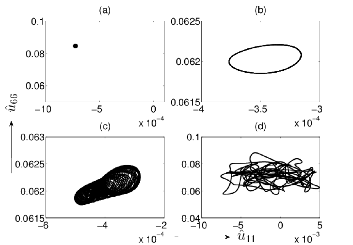
We use the amplitude of the Fourier mode to distinguish the regimes discussed above. To further quantify the dynamics, in Fig. 3 we plot the phase space projection along the and axes. For and , Fig. 3(a) shows a stationary state with . It corresponds to the pattern displayed in Fig. 2(b). These stationary states are located using right triangles in Fig. 1. As described above, they are generated either by a pitchfork bifurcation from the linear flow regime or by a more complex sequence of bifurcations [thess:1992]. A further increase of to leads to a limit cycle generated through a supercritical Hopf bifurcation and displayed in Fig. 3(b). The corresponding spatial pattern is shown in Fig. 2(c). In Fig. 1, these limit cycles are shown using (). For , another Hopf (to be precise Neimark-Sacker) bifurcation yields a quasi-periodic state, as illustrated in Fig. 3(c). The spatial pattern is displayed in Fig. 2(d)). These states are located using downward triangles in Fig. 1. This regime becomes chaotic when is slightly increased ().
A further increase of () changes the system behavior to another kind of chaotic attractor, which is larger and symmetric in , as shown in Fig. 3(d). For these regimes, the mean value of vanishes, and the reflection symmetry with respect to and is statistically restored (compared to the attractor of Fig. 3(c)). These patterns are shown using squares in Fig. 1. A similar sequence of bifurcations from the linear flow to a chaotic regime is observed in experiments [herault:2013].

The power spectral densities of the large scale mode related to the periodic, quasiperiodic, and chaotic regimes described above are displayed in Fig. 4. The limit cycle for involves a fundamental frequency together with its harmonics (see Fig. 4(a)). The power spectrum for the quasiperiodic state corresponding to involves another frequency and the linear combinations of and (see Fig. 4(b)). These peaks become enlarged by an increasing amount of low frequency noise as displayed in Fig. 4(c) that corresponds to a chaotic regime with a non zero mean flow (). As is increased further, the two symmetric attractors merge, and a fully chaotic regime with zero mean flow is obtained (Fig. 4(d) for ). The noise level displays an exponential decay as a function of frequency.

A similar sequence of bifurcations is observed when we increase at fixed (horizontal arrow in Fig.1). The linear response to the spatial forcing is stable for (Fig. 5(a)). When is increased, the flow bifurcates to another stationary flow that involves modes other than (6,6), in particular the large scale mode (see Fig. 5(b)). Further increase of yields successive bifurcations to time-periodic and chaotic flows with non zero large scale flow. The large scale mode becomes more and more important as is increased further(see Fig. 5(c, d)).
In the next subsection we will describe how new patterns emerge when is increased beyond the chaotic regime.
III.2 Transition from chaotic to condensate states
In the previous subsection, we discussed in detail the system dynamics for to 10 with . We obtained patterns corresponding to fixed point, periodic, quasiperiodic, and chaotic states. For the chaotic state at , the large scale velocity mode randomly changes sign, as depicted in the time series of Fig. 6(a) (corresponding to Fig. 2(e)). The probability density function (PDF) of is displayed in Fig. 7. It is close to a gaussian with a maximum for .
As is increased further to 30, fluctuates more strongly, as evident from the time series of Fig. 6(b). More importantly, the PDF of exhibits two peaks at as shown in Fig. 7. This transition from a gaussian with a mean value to a double-peaked symmetric PDF when is increased can be considered as the low border of the reversal regime.
A further increase of to 50 shows the chaotically reversing regime more clearly, as illustrated in Fig. 6(c). The maximum of the PDF of occurs at larger . In addition, the residence time in one of the states with opposite large scale circulations becomes much longer than the eddy turn-over time. The average residence time increases when is increased further.
Finally, when , the large scale circulation no longer changes sign, and a “condensed” state is obtained (see Fig. 6(d)). The large scale circulation displays intermittent fluctuations around a mean nonzero value of . The flow pattern of a condensed state is shown in Figs. 2(f) and 5(c,d). In Fig. 7, we plot the PDF of for , which shows fluctuations around a positive , consistent with the time series depicted in Fig. 6(d). In the condensed state, the attractors corresponding to both directions of the large scale circulation are disconnected in phase space.
The aforementioned condensed state has been attributed to the inverse cascade of energy from the forcing scale to the largest possible scale [kraichnan:1967]. Another viewpoint has been put forward recently by Gallet and Young [gallet:2013]. They found the condensate as an approximate nonlinear solution of Eq. (1) in the absence of friction (). For the forcing, the condensate is generated through a pitchfork bifurcation from the linear flow regime as is increased, and it stays stationary up to . It is evident from our simulations that the large scale mode starts playing a major role as soon as the linear response to the forcing becomes unstable, and this mode is used to characterize the different flow regimes.
Our simulations illustrate that for , the mode is dominant in the limit of large which corresponds to a small dissipation rate at large scales. It is interesting to observe how the condensate disappears when is decreased. We observe in Fig. 1 that it bifurcates to a regime with random reversals of the large scale circulation and then to the chaotic regime with zero mean flow.


IV Energy budget
The aforementioned dynamical regimes involve energy exchanges among the Fourier modes due to nonlinear interactions. These interactions generate energy transfer from the injected power by the periodic forcing to the small-scale viscous dissipation and the large-scale drag. An integration over space of the scalar product of Eq. (1) with the velocity yields the following equation for the energy budget:
| (13) |
where
| (14) |
is the kinetic energy,
| (15) |
is the injected power (note that because of incompressibility),
| (16) |
is the large scale dissipation, and
| (17) |
is the small scale viscous dissipation. Note that is most active at small length scales, while is most active at large length scales since is strongest at large scales.
In a statistically stationary regime, we obtain
| (18) |
where stands for the time average.

In Fig. 8, we plot , and versus for , and . We first observe that the mean injected power decreases when is increased. This is in agreement with the mechanism proposed by Tsang and Young [tsang:2009]; the advection of the vortices at the forcing scale by the large scale flow detunes the vortices from the spatial forcing thus decreasing its efficiency. As the energy of the large scale flow increases with (Fig. 8 and Fig. 9), the detuning of the forcing becomes stronger, thus leading to the decrease of .
This mechanism operates here even though the present simulations are not in a regime in which viscous dissipation is negligible compared to the large scale drag. This regime was achieved in reference [tsang:2009] since the scale separation between the forcing scale and the box scale was much larger than in our simulations and hyperviscosity was used. In our case, mean viscous dissipation and large scale drag are of the same order in the chaotic regimes when and . For , becomes large compared to for the largest values of .
An interesting trend displayed in Fig. 8 is the relative magnitude of with respect to when is varied. For , the linear response to the forcing is stable and one expects when is large. When is increased and the flow becomes chaotic, one observes that first increases whereas decreases. The value of for which they become equal increases with .
As described above, our simulations are not performed in a turbulent regime for which that would correspond to the two-dimensional turbulence phenomenology in which the injected power cascades to large scales and is mostly dissipated by large scale drag. Only for the largest Reynolds number, , we have a few times larger than for but their ratio is of order one for . We expect that will be larger for which is the value of the Reynolds number reached in the experiments [sommeria:1986, herault:2013]. Increasing scale separation between the forcing and the box size will also allow the development of the inverse cascade, thus increasing . However, even though our simulations are not conducted in this regime, the condensed state predicted by two- dimensional turbulence is well observed.

The normalized energy (respectively ) of the mode (respectively ) is displayed versus for , and in Fig. 9. We define and where is the kinetic energy of the flow. strongly decreases when is increased such that the linear response to the forcing becomes unstable, while increases. As said above, this phenomenon is observed even though we are not in a regime with a well developed inverse cascade with .

The temporal cross-correlation between the injected power and the kinetic energy , , and the temporal cross-correlation between and the viscous dissipation , , are displayed in Fig. 10. The correlation reach unity in the chaotic regime with zero mean (, see Fig. 10(a)). The maximum of the correlation decreases as is increased, because the flow is much more disordered in space for or (reversal regime) than for . For these values of , the cross-correlation of injected power with small scale dissipation is larger than the correlation of injected power with large scale dissipation since (Fig. 10(b, c)). In the condensed state, the opposite is observed (Fig. 10(d)). The maximum of the cross-correlation is for positive time lag , thus kinetic energy or large scale dissipation and viscous dissipation lag behind injected power. In the turbulent regimes ( or ), the time lag is of the order of one eddy turn-over time.
V Reversals of the large-scale circulation (LSC)
As described in earlier sections, random reversals of the LSC are observed for and intermediate values of in a rather extended domain of (-) parameter space (Fig. 1). These reversals regimes are illustrated in Fig. 6(c) using the time series of and plotted in Fig. 1 using (). The PDF of displayed in Fig. 7 shows two maxima at for the reversal states.

Fig. 11 shows time series of , injected power , kinetic energy , and viscous dissipation for and . Besides reversals, one also observes excursions or aborted reversals for which the amplitude of starts decreasing as if a reversal were initiated, but the flow then comes back to the state with the same sign of instead of reversing. The value of increases somewhat during the reversals. The high energy state (during the transition) is associated with a larger dissipation at large scale, and is also related to higher levels of injected power and viscous dissipation . Thus, , , , and exhibit small spikes during reversals and excursions (see below).
In Fig. 12(a,b) we present the phase-space projection - for and . For , the low energy state corresponds to the dense lobes at the bottom of the attractor. The high energy state, which also corresponds to a larger injected power, i.e. a larger mean value of , corresponds the regions with medium density. Only these regions are connected by trajectories corresponding to reversals. For and , the two dense lobes get disconnected and become the condensed state. The presence of low and high energy injection states, corresponding respectively to high and low amplitudes of , is in good agreement with the saturation mechanism mentioned above.
For , the low energy state no longer exists (see Fig. 12(b)). The mode reverses between positive and negative values, but the peak of the PDF is lower than that for . Similar features involving two turbulent states with different level of fluctuations in relation with condensation have been described in experiments [shats:2005].


Further information about the statistical properties of the low and high energy states can be obtained from the PDF displayed in Fig. 13. The PDFs of show symmetric fluctuations about the mean in both states. In contrast, the PDF of the injected power is roughly Gaussian in the high energy state whereas it is asymmetric with an exponential tail toward large values in the low energy state. A similar trend is observed for the PDF of viscous dissipation . The PDFs of the low energy state have a similar shape to the ones of the condensed state.

Next we consider the time series of some of the dominant modes during a reversal of the LSC in Fig. 14. We plot the time series of , , , and . Clearly, mode switches sign, while the mode does not change sign. The other modes display large fluctuations compared to their mean value. However, we observe that the mode keeps a positive mean. This trend is not observed for the modes and which exhibit their strongest fluctuations during the reversal.
In Appendix B we classify the reversing modes based on group theoretic arguments, and show that the Fourier modes (even, even), (odd, odd), (even, odd), (odd, even) should behave during reversals according to a small number of possible scenarios. One of them is: ; ; . That is, the even modes do not change sign, the odd modes change sign, and the mixed modes and have zero mean. A similar feature has been observed for the flow reversals in two-dimensional turbulent convection: all the odd modes (e.g., , etc.) change sign, while the even modes (e.g., ) keep the same sign [chandra:2011, chandra:2013]. However, in the present study, these possible scenarios are blurred by strong turbulent fluctuations.
Gallet et al. [gallet:2012] studied the evolution of , , and modes using numerical simulations, and obtained similar results, that is, reverses, but and fluctuate around zero, with strong fluctuations during a reversal. Gallet et al. [gallet:2012] based their arguments on reflection symmetries about and axes passing through the centre of the box. The symmetry arguments of Gallet et al. [gallet:2012] and those given in the appendix are equivalent.
Gallet et al. [gallet:2012] proposed a low dimensional model of reversals of the LSC driven by a forcing using the modes (1,2) and (2,1) which have a quadrupolar like symmetry interacting with the large scale mode (1,1) which has a dipolar like symmetry. The possible triad through which (1,2), (2,1) and (1,1) could interact is [(1,2), (2,1), (1,1)]. However, this interaction is forbidden due to the symmetry of (1,1) mode under a rotation by . A closer inspection shows that the interacting triads responsible for reversals are and .

The flow structure at various stages during the reversal is shown in Fig. 15. The vorticity levels are represented with different colors and the velocity field is indicated with arrows. Fig. 15(a) shows the LSC rotating in the counterclockwise direction. The single eddy breaks into four eddies as shown in Fig. 15(b). This structure is followed transiently by two-eddy structures (Fig. 15(b-e)). Finally the upper eddy starts pushing the lower one and a single eddy rotating clockwise occupies the box (see Fig. 15(f)). Thus this suggests to be a possible sequence of the flow structures during the reversal.
VI Transition from the reversal regime to the condensate state
As we increase , the flow stops reversing beyond some , and we observe a condensate state. The condensed states are exhibited in Fig. 1 using (), and their flow profile is displayed in Figs. 2(f) and 5(c,d).
As discussed in the previous section, for small , flow reversals occurs due to nonlinear interactions among the modes of the triads and the triad . For the reversal, it is critical that the secondary mode be of significant strength. We compute this ratio and plot it as a function of for , and in Fig. 16. We observe that the ratio decreases with increasing , and it is very small () for large . This is the reason why reversals stop at large , and we obtain a condensate state. Note that the relative strengthening of mode compared to the secondary modes occurs due to an inverse cascade of energy. Very similar phenomena was observed by Chandra and Verma [chandra:2011, chandra:2013] for thermal convection in two-dimensional box geometry; the reversal stopped at large Rayleigh number due to small value of the ratio .


The phase space projection on the modes - shown in Fig. 17 compares the attractor related to the condensate state (in black) to the one related to the reversal regime (in grey). The fluctuations in the condensed state increase when is increased. For , the attractor corresponding to the low energy state of the reversal regime transforms into the attractor of the condensate.
Finally, it is instructive to consider the cross-correlation between the injected power and the kinetic energy of the large scale mode in the reversal regime and the condensate state. Fig. 18 shows that the large scale flow and the injected power are anticorrelated, i.e. the cross-correlation reaches large negative values for some time lag. This is in agreement with the mechanism proposed by Tsang and Young [tsang:2009] in which the large scale flow detunes the small scale pattern from the forcing thus decreasing the injected power. However, the sign of the time lag changes with . In the reversal regime, it is positive, thus the kinetic energy of the large scale mode lags behind the injected power. Consequently, reversals may result from fluctuations in the energy budget. The opposite is observed in the condensate state for which the injected power lags behind the large scale flow. Detuning induced by the large scale flow controls the injected power.

As described above, the condensate state has been predicted in the framework of two-dimensional turbulence phenomenology [kraichnan:1967]. Its observation in direct numerical simulations has been first performed using the two-dimensional Navier-Stokes equation without large scale drag and using hyperviscosity to regularize the small scales [smith:1993, chertkov:2007]. In addition, the forcing was applied at small scale with respect to the box size and consists of white noise. The later provides a constant injected power and scale separation and hyperviscosity allow a well developed inverse cascade of energy. We have shown here that a condensate can be obtained even when both the large scale drag and small scale viscous dissipation play a significant role in the energy budget. A different approach for the condensed state has been recently provided by showing that it can be understood has a nonlinear solution of the two-dimensional Navier-Stokes equation without large scale drag. In the limit , the LSC detunes the linear response to the constant and spatially periodic forcing, such that the injected power becomes vanishingly small [gallet:2013]. This approach strongly differs from the phenomenology of two-dimensional turbulence as far as the injected power is concerned. It looks to fit better with the flow configuration we studied in this work.
VII Conclusions
We performed a numerical study of a two-dimensional Kolmogorov flow generated by a spatially periodic and constant force and linearly damped by a drag force with a decay rate . When the Reynolds number or are small, the linear response to the forcing is stable, and the system takes the form of a square arrays of alternate counter-rotating vortices. We studied variation of patterns for various and , but focussed on varying for a particular , more specifically . When was increased, the flow becomes unstable, and it follows a sequence of transitions to a fixed point, periodic, quasiperiodic, and chaotic states. The most dominant Fourier mode that represents the large-scale flow describes the aforementioned states very well.
We observed two kinds of chaotic states: a first one with a nonzero mean value of , and the second one with a zero mean value of . The second chaotic state occurs for larger . On further increase of , the PDF of the mode transitions from a gaussian distribution to a bimodal distribution. The maxima of the bimodal distribution are related to LSC with opposite values of the velocity. The distribution becomes more and more peaked as is increased, thus leading to flow reversals, in which the mode randomly switches between two quasi-stationary states.
A further increase in to around 100 leads to cessation of flow reversals, and we obtain a condensate state in which the flow moves continuously in one direction. We attribute the condensate state to weakening of the secondary mode that plays a very critical role in the flow reversal. The relative strengthening of over the secondary modes is due to the inverse cascade of energy in two-dimensional flow.
Very similar phenomena were observed by Chandra and Verma [chandra:2011, chandra:2013] for turbulent convection in a two-dimensional square box. They obtained flow reversals after a series of bifurcations, as the Rayleigh number was increased. However, the flow reversals stopped for very large Rayleigh number due to weakening of the secondary mode . Chandra and Verma [chandra:2011, chandra:2013] argue that the most dominant triads responsible for the flow reversals in turbulent convection are and , which appears to be the same in the Kolmogorov flow discussed in this paper.
All these transitions are in fair agreement with experimental observations [sommeria:1986, herault:2013] thus showing that the two-dimensional modeling of the flow with stress-free boundary conditions is a reasonable approximation. Taking into account rigid boundary conditions can be important in the absence of large scale drag () when reversals are generated by random forcing [molenaar:2004, vanheijst:2006]. In that case, it has been found that reversals are induced by generation of vorticity in the lateral boundary layers. However, this does not correspond to the experimental configurations quoted above or to our numerical simulations.
Reversals of a vector field are widely observed in geophysics or astrophysics. The so-called quasi-biennial oscillation is an example of a large scale almost cyclic reversing flow in the turbulent atmosphere. It is a roughly periodic oscillation in the strength and direction of the zonal (east-west) wind in the lower and middle stratosphere over the equator of the Earth’s atmosphere [baldwin:2001]. The magnetic field of the Earth and the sun also display random (respectively roughly periodic) reversals. Reversals of a large scale velocity field over a turbulent background in thermal convection [sugiyama:2010, chandra:2011, chandra:2013] or of a magnetic field generated through the dynamo effect by a von Karman swirling flow [berhanu:2010] have been studied in the past years in laboratory experiments. Although the dynamo experiment involves flows with much larger turbulent fluctuations than the convection experiment or the Kolmogorov flow, it has been found that reversals of the magnetic field follow well defined trajectories in phase space (see Fig. 7 in [berhanu:2010]). This clearly differs from the reversals studied here (see Fig. 12). Although we have identified some intermediate structures that correspond to the Fourier, modes (2,1), (1,2) and (2,2) during reversals, it seems unlikely that low dimensional models similar to the ones designed for reversals of the magnetic field [petrelis:2008, petrelis:2010] can capture all the features of reversals of the LSC in Kolmogorov flows. Turbulent fluctuations are difficult to disentangle from the dynamics of the dominant modes in the present situation, such that a different approach should be found to describe these bifurcations between different turbulent regimes.
Appendix A Energy transfers among Fourier modes in Kolmogorov flows
As described in Sec. II, we force the Fourier mode, hence the energy input to the system is via this mode. The nonlinearity however enables energy transfers to other modes. In this paper we focus on the energy transfer to the (1,1) mode, which contributes most significantly to the large-scale circulation (LSC).
The equation for the energy of a mode is
| (19) |
where are the Fourier component of the velocity, is the Fourier component of the force, and is the rate of energy transfer into mode from all other modes via nonlinear triad interactions. Dar et al. [dar:2001] and Verma [verma:2004] showed that
| (20) |
with , and
| (21) |
is the “mode-to-mode energy transfer” from mode to with acting as a mediator. Note that is a real vector. Using the incompressibility condition [Eq. (2)], the above expression becomes
| (22) |
The above expression for the mode-to-mode energy transfer is very useful. We can deduce the energy transfer rate from the mode to the mode using this formula. Clearly, and form two important triads for the above energy transfers. Hence,
| (23) |