Antagonistic in-plane resistivity anisotropies from competing fluctuations in underdoped cuprates

The existence of a sizable in-plane electronic anisotropy in different families of underdoped cuprates has been established by a variety of experimental probes, such as transport measurements [1, 2, 3], x-ray [4, 5] and neutron scattering [6, 7], and scanning tunneling microscopy [8]. Consonant with the proposal of electronic nematic order [9, 10, 11, 12], in which the point group symmetry of the system is lowered spontaneously by electronic degrees of freedom, these experiments provide invaluable information for the hotly debated topic of whether any symmetries are broken in the pseudogap phase [13, 14]. To elucidate the relevance of these anisotropic properties to the phase diagram of the cuprates, it is fundamental to establish their microscopic origin. In this regard, a useful benchmark for theoretical proposals is the in-plane resistivity anisotropy $\Delta\rho\equiv\left(\rho_{a}-\rho_{b}\right)/\rho_{b}$, which was measured in the seminal work [1] across the phase diagram of YBa₂Cu₃O₇ (YBCO). The moderate values of the resistivity anisotropy that were observed experimentally, $\Delta\rho\lesssim 1.5$, are difficult to reconcile with a scenario in which metallic static stripes [15, 16] order in an insulating background. Instead, they seem to be more compatible with fluctuations that break the tetragonal symmetry of the system [10, 17].

Interestingly, neutron and x-ray measurements in underdoped YBCO have unveiled the onset of anisotropic charge and spin fluctuations at temperatures comparable to those marking the onset of $\Delta\rho$. Refs. [6, 7] found that the dynamic spin susceptibility $\chi_{\mathrm{S}}\left(\mathbf{q},\omega\right)$ in the vicinity of the magnetic ordering vector $\mathbf{Q}_{S}=\left(\pi,\pi\right)$ becomes strongly anisotropic as temperature is lowered, eventually giving rise to incommensurate peaks along the $a$ direction only, and to long-range spin-density wave (SDW) order at low temperatures. More recently, it was reported that the charge susceptibility $\chi_{\mathrm{C}}\left(\mathbf{q},\omega\right)$ is also anisotropic, with fluctuations peaked at the ordering vector $\mathbf{Q}_{C,b}=Q_{C}\hat{\mathbf{b}}$ stronger than the fluctuations peaked at the $90^{\circ}$-rotated ordering vector $\mathbf{Q}_{C,a}=Q_{C}\hat{\mathbf{a}}$ [18, 19, 4, 5]. At high magnetic fields, superconductivity is destroyed and these fluctuations are believed to give rise to charge-density wave (CDW) order [20, 21]. Interestingly, the SDW and CDW fluctuations seem anti-correlated in the phase diagram of YBCO [19, 4] (see Fig. 1): while the anisotropic spin fluctuations dominate the hole-doping concentration range $0.05\lesssim p\lesssim 0.08$, the anisotropic charge fluctuations are observed predominantly in the $0.09\lesssim p\lesssim 0.13$ range.

In this paper, we calculate the resistivity anisotropy due to the scattering by the anisotropic charge and spin fluctuations observed in Refs. [6, 4, 5] and compare it qualitatively with the resistivity anisotropy measurements of Ref. [1]. Because our focus is on the sign of $\Delta\rho\equiv\left(\rho_{a}-\rho_{b}\right)/\rho_{b}$ and on its dependence on the charge and spin correlation lengths $\xi_{C}$ and $\xi_{S}$, respectively, we employ a Boltzmann equation approach. We find that while scattering by charge fluctuations yields $\Delta\rho<0$ and $\left|\Delta\rho\right|\propto\xi_{C}^{2}$ , scattering by spin fluctuations gives $\Delta\rho>0$ and $\left|\Delta\rho\right|\propto\ln\xi_{S}$. These different behaviors arise from the fact that the former is governed by the Fermi velocity at the CDW hot spots, whereas the latter is sensitive to the curvature of the Fermi surface near the SDW hot spots. We discuss the key role played by the CuO chains present in YBCO, which act effectively as a conjugate field to the nematic order parameter, selecting the experimentally-observed fluctuation anisotropies. Our findings are consistent with the resistivity anisotropy measurements in YBCO, and in particular with the doping dependence of $\Delta\rho$ in the range $0.05\lesssim p\lesssim 0.15$.

Our focus here is not on the mechanism responsible for the anisotropic CDW and SDW fluctuations – in fact, several models for nematicity in the cuprates have been proposed [9, 22, 23, 24, 25, 26, 27, 28, 29, 30]. Instead, we assume spontaneous nematic order and adopt a phenomenological approach in which the low-energy properties of the CDW and SDW susceptibilities are extracted from the scattering experiments [6, 4, 5]. Following previous works [31, 32, 33, 34, 29], we consider the CDW ordering vectors $\mathbf{Q}_{C,i}$ that connect the magnetic hot spots of the Fermi surface [35], according to Fig. 2. We note however that small changes in the positions of the CDW hot spots do not affect our conclusions. Because $\mathbf{Q}_{C,i}$ and $\mathbf{Q}_{S}$ connect states at the Fermi level, the CDW and SDW dynamics are dominated by Landau damping, i.e. $\chi_{\alpha}^{-1}\left(\mathbf{q},\omega\right)=\chi_{\alpha}^{-1}\left(\mathbf{q}\right)-i\omega/\Gamma_{\alpha}$ and $\alpha=C,S$, with $\Gamma_{C/S}\propto v_{F}Q_{C/S}$, where $v_{F}$ is the Fermi velocity. The anisotropy of the fluctuations is manifested in their static components, which, according to the experimental observations, can be modeled as:

where the upper (lower) sign in the first equation refers to $i=a$ ($i=b$). Hereafter, $\hat{\mathbf{x}}\parallel\hat{\mathbf{a}}$, $\hat{\mathbf{y}}\parallel\hat{\mathbf{b}}$, and all lengths are measured in units of the lattice constant. Fig. 2 displays the contour plots of the susceptibilities, highlighting their anisotropic features: while the anisotropy of the CDW fluctuations is manifested as different correlation lengths [29, 36, 37], $\eta_{C}=\left(\xi_{C,a}^{-2}-\xi_{C,b}^{-2}\right)/2\xi_{C}^{-2}$, the anisotropy of the SDW fluctuations is manifested only on its form factor via the dimensionless parameter $\eta_{S}$. When $\left|\eta_{S}\right|>1$, the SDW develops an incommensurability along either $a$ ($\eta_{S}<0$) or $b$ ($\eta_{S}>0$). Thus, both $\eta_{S}$ and $\eta_{C}$ are Ising-nematic order parameters and the anisotropic resistivity obeys, by symmetry, $\Delta\rho=C_{S}\eta_{S}+C_{C}\eta_{C}$. Because our main goal is to establish the sign of the pre-factors $C_{S}$ and $C_{C}$, hereafter we consider the regime $\eta_{S,C}\ll 1$.

Because macroscopic samples will be divided in equal-weight domains of $\eta_{S,C}$ and $-\eta_{S,C}$, one would not expect to observe anisotropic properties which average over the entire sample, such as $\Delta\rho$. This issue can be avoided if fields that explicitly break the tetragonal symmetry and select one domain over the other are present. In terms of a Ginzburg-Landau functional, they can be recast in terms of the conjugate fields $h_{C}$ and $h_{S}$:

where the functional $F_{0}$ depends only on even powers of $\eta_{S,C}^{2}$ and $\eta_{S}\eta_{C}$. In tetragonal cuprates such as HgBa₂CuO₄ and Nd₂CuO₄ the symmetry-breaking field needs to be externally applied in the form of uniaxial strain. However, in detwinned YBCO, the presence of unidirectional CuO chains makes it orthorhombic, with the $b$ direction parallel to the CuO chains [38, 39]. Thus, the small orthorhombic distortion acts effectively as an external field that selects one type of domain [40].

To verify whether this picture correctly captures the signs of $\eta_{S}$ and $\eta_{C}$ observed experimentally in YBCO, namely $\eta_{S}<0$ and $\eta_{C}>0$, we computed the signs of the effective fields $h_{C,S}$ generated by the coupling between the CuO chains and the CuO₂ planes via evaluation of the non-interacting polarization bubble $\Pi(\mathbf{q},\omega)$ for a tight-binding model containing the chains and the planes [38, 39] (see supplementary material¹¹ 1 See Supplemental Material [url], which includes Refs.[39, 33, 38, 57, 42, 43]). Because the contribution of the chains to the susceptibilities (1) is given by $\tilde{\chi}_{\alpha}^{-1}\left(\mathbf{q}\right)-\chi_{\alpha}^{-1}\left(\mathbf{q}\right)=-\Pi\left(\mathbf{q}\right)$, where $\tilde{\chi}$ is the susceptibility in the presence of the conjugate fields induced by the chains, it is straightforward to extract the fields $h_{C,S}$. In Fig. 3 we plot $\Pi\left(\mathbf{q}\right)$ across the first Brillouin zone, and present in the inset cuts along the high-symmetry directions $\left(q_{x},0\right)$, $\left(0,q_{y}\right)$, $\left(\pi+q_{x},\pi\right)$ and $\left(\pi,\pi+q_{y}\right)$.

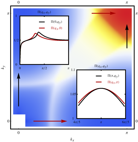
First, we note that the peaks along the $90^{\circ}$-related cuts $\Pi\left(q_{x},0\right)$ and $\Pi\left(0,q_{y}\right)$ are different, with the peak along the $q_{y}$ axis (parallel to $b$) stronger, which corresponds to a larger correlation length around the $\mathbf{Q}_{C,b}$ ordering vector, $\xi_{C,b}>\xi_{C,a}$. Therefore, the effect of the chains can be recast in terms of a positive conjugate field $h_{C}>0$ that selects the $\eta_{C}>0$ domain, in agreement with the x-ray observations in YBCO [4, 5]. Meanwhile, a cut along the $a$ and $b$ axes centered at the $\mathbf{Q}_{S}=\left(\pi,\pi\right)$ ordering vector gives $\Pi\left(\pi+q_{x},\pi\right)-\Pi\left(\pi,\pi\right)=-\alpha_{x}q_{x}^{2}$ and $\Pi\left(\pi,\pi+q_{y}\right)-\Pi\left(\pi,\pi\right)=-\alpha_{y}q_{y}^{2}$, with $\alpha_{x}<\alpha_{y}$. Thus, comparison with Eqs. (1) reveals that the chains act as a negative conjugate field $h_{S}<0$, which selects the $\eta_{S}<0$ domain, as also observed experimentally in YBCO via neutron scattering [6, 7]. Note that, as pointed out in Ref. [1], even though the chains contribute to $\Delta\rho$, they cannot alone explain the resistivity anisotropy behavior, since $\Delta\rho$ has a non-monotonic variation as doping decreases, whereas the degree of chain order decreases continuously with decreasing $p$.

Having established the form of the anisotropic SDW and CDW susceptibilities, we now compute the resistivity anisotropy arising from the scattering of electrons by these fluctuations. Because we focus on the sign of $\Delta\rho$ for small $\eta_{C,S}$, it is appropriate to employ a semi-classical Boltzmann approach [42, 43, 44], since the smallness of $\eta_{C,S}$ allows for a perturbative treatment of the collision kernel, even if the SDW and CDW coupling constants are not necessarily small. Furthermore, the observations of quantum oscillations [2], of a $T^{2}$ behavior in the resistivity [45], of the validity of Kohler’s rule [46], and of a $\omega^{2}$ behavior in the ac conductivity [47] suggest that quasi-particles are well-defined in the doping range of interest. We emphasize that our focus is in the underdoped regime where $\xi_{S,C}$ remains finite, and the system is near a finite-temperature nematic phase transition. Near a putative nematic quantum critical point, the quasi-particle concept is compromised, and other approaches may be more appropriate [48, 49, 50].

Besides the inelastic scattering by CDW and SDW fluctuations, electrons are also scattered elastically by impurities (see also Refs. [51, 52]). Here, we consider the limit where the impurity potential provides the dominant scattering mechanism, which is always true at low enough temperatures. Alternatively, similar results can be obtained in the limit where scattering by isotropic fluctuations is dominant. We avoid the extremely low-temperature regime, where weak-localization and Fermi-velocity renormalization effects may be important. In the impurity-dominated regime [42, 43], the solution of the Boltzmann equation yields the resistivity anisotropy (see supplementary material):

with the collision integrals:

and the kernels:

Here, $\alpha=C_{a},C_{b},S$ refers to the CDW fluctuations around the ordering vectors $\mathbf{Q}_{C,a/b}$ and to the SDW fluctuations around $\mathbf{Q}_{S}$. $h_{j}=\frac{\tau e\beta}{\hbar}\,\frac{\partial\varepsilon_{\mathbf{k}}}{\partial k_{j}}$, with $i=x,y$, denotes the deviation of the electronic distribution function $n_{F}$ from the equilibrium Fermi-Dirac distribution $n_{F}^{0}$ in the presence of an electric field $\mathbf{E}$, $n_{F}=n_{F}^{0}-\beta^{-1}\left(\partial_{\epsilon}n_{F}^{0}\right)\mathbf{h}\cdot\mathbf{E}$, $\tau^{-1}=g_{0}^{2}/(\pi\nu_{F}\hbar)$ is the impurity scattering rate and $\rho_{0}=\frac{\hbar}{e^{2}}\frac{2\pi}{\hbar\nu_{F}\tau}\frac{1}{\braket{v_{j}^{2}}_{\hat{k}}}$ is the impurity-induced residual resistivity. The electronic dispersion is denoted by $\varepsilon_{\mathbf{p}}$, the CDW and SDW susceptibilities $\chi_{\alpha}$ are given by Eq. (1) and $g_{0}$, $g_{\alpha}$ denote the scattering amplitudes for impurities and fluctuations, respectively.

The collision integrals that determine the resistivity anisotropy (4) are dominated by their behavior near the CDW/SDW hot spots, $\varepsilon_{\mathbf{p}+\mathbf{Q}_{\alpha}}=\varepsilon_{\mathbf{p}}=0$, where the susceptibility $\chi_{\alpha}$ is the largest. For the CDW fluctuations, Eq. (1), because the anisotropy is manifested in the correlation length we find that the anisotropy depends only on the Fermi velocity at the hot spots. Introducing the average distance between thermally induced fluctuations $\xi_{T}=\sqrt{\frac{3\Gamma_{C}\beta}{2\pi}}$, we obtain in the low-temperature limit $\xi_{T}\gg\xi_{C}\gg 1$ the leading-order expression:

where $\chi_{0,C}^{-1}$ is the CDW energy scale and $C_{C}<0$ is a dimensionless positive constant that depends only on the Fermi velocity at the CDW hot spots. Therefore, in YBCO, since $\eta_{C}>0$, scattering by charge fluctuations favor $\rho_{a}<\rho_{b}$. This can be understood in the following way: since $\eta_{C}>0$, fluctuations are stronger around the $\mathbf{Q}_{C,b}$ CDW ordering vector, i.e. $\xi_{C,b}>\xi_{C,a}$. As shown in Fig. 2, at the hot spots connected by $\mathbf{Q}_{C,b}$, the Fermi velocity is almost parallel to the $b$ axis. Thus, electrons moving along the $b$ direction experience enhanced scattering compared to the electrons moving along $a$, causing $\rho_{a}<\rho_{b}$. This argument makes it clear that small deviations in the value of $Q_{C}$ do not change the result.

As for the SDW fluctuations, the anisotropy does not arise from the ordering vector $\mathbf{Q}_{S}=(\pi,\pi)$, which is isotropic, but from the form factor. As a result, defining again $\xi_{T}=\sqrt{\frac{3\Gamma_{S}\beta}{2\pi}}$ and focusing in the regime $\xi_{T}\gg\xi_{S}\gg 1$, we obtain:

In contrast to the CDW case, the dimensionless pre-factor $C_{\mathrm{S}}$ depends on the curvature of the Fermi surface and on the derivatives of the Fermi velocity near the hot spots. As a result, $C_{S}$ may depend on additional details of the Fermi surface, as compared to $C_{C}$. We computed it using two different sets of tight-binding parameters [39, 33] and different values of the chemical potential, finding that in general $C_{S}<0$. Consequently, since $\eta_{S}<0$ in YBCO, scattering by SDW fluctuations yields $\rho_{a}>\rho_{b}$. This can be understood as a consequence of the fact that the SDW fluctuations stiffness is smaller along the $a$ axis, since $\eta_{S}<0$ in Eq. (1), which enhances the scattering along this direction. Note that, because long-range SDW order is present while long-range CDW order is absent in the underdoped phase diagram, $\xi_{S}$ can become very large whereas $\xi_{C}$ remains bounded.

We now contrast our results to the experimental measurements of $\Delta\rho\equiv\left(\rho_{a}-\rho_{b}\right)/\rho_{b}$ [1]. In YBCO, the CuO chains, parallel to the $b$ axis, give an intrinsic contribution to the resistivity anisotropy, $\Delta\rho_{\mathrm{chain}}>0$ (see dashed line in Fig. 4). Thus, the contribution from the CDW/SDW fluctuations add to or subtract from this intrinsic background. As shown in the inset of Fig. 4, anisotropic SDW and CDW fluctuations compete and dominate different regions of the underdoped phase diagram. Starting at $p\approx 0.05$ and increasing $p$, the anisotropic SDW fluctuations with $\eta_{S}<0$ are suppressed as the corresponding transition line disappears near $p\approx 0.08$ [5, 4]. According to our results, $\Delta\rho$ should be positive and should decrease as $p$ increases and $\xi_{S}$ is suppressed, as shown by the arrow in Fig. 4. This behavior is indeed observed experimentally [1]. CDW fluctuations emerge at $p\approx 0.09$ – initially they are anisotropic, with $\eta_{C}>0$, but as $p\approx 0.13$ is approached they become isotropic [5], with $\eta_{C}\rightarrow 0$. In this regime, we find that the anisotropic CDW fluctuations give $\Delta\rho<0$. Experimentally, the measured $\Delta\rho$ remains positive in this region, but is the smallest in the phase diagram [1], which could be understood as a consequence of $\Delta\rho<0$ appearing on the intrisinc $\Delta\rho_{\mathrm{chain}}>0$ background. To shed light on this issue and disentangle the chains contribution, it would be desirable to perform transport measurements in tetragonal compounds such as HgBa₂CuO₄ and Nd₂CuO₄, where CDW fluctuations have also been reported [53, 54]. In this case, application of uniaxial strain [55, 56] would be necessary to select a single nematic domain. Note that for very underdoped YBCO samples, long-range SDW order sets in at very low temperatures [7], giving rise to an anisotropic reconstructed Fermi surface, which promote a non-zero $\Delta\rho$ even in the absence of inelastic scattering at $T=0$.

In summary, we have shown that the anisotropic charge and spin fluctuations present in YBCO give antagonistic contributions to the resistivity anisotropy in underdoped cuprates. While the SDW fluctuations provide a plausible explanation for the resistivity anisotropy observed experimentally, the contribution of CDW fluctuations seems to be nearly cancelled by the contribution coming from the CuO chains. An open issue is how these anisotropic fluctuations affect other anisotropic transport quantities, such as the thermopower and the Nernst anisotropy [2]. Although a non-zero $\Delta\rho$ is not surprising, since these fluctuations are $C_{2}$ symmetric, the fact that the competing fluctuating channels promote different signs for $\Delta\rho$ is unanticipated, opening a promising route to disentangle the contributions from spin and charge degrees of freedom to the formation of the nematic state observed in underdoped cuprates.

We thank M. Chan, A. Chubukov, M. Greven, M. Le Tacon, and J. Schmalian for fruitful discussions. MS acknowledges the support from the Humboldt Foundation. RMF is supported by the U.S. Department of Energy under Award Number DE-SC0012336.

References

- [1] Y. Ando, K. Segawa, S. Komiya, and A. N. Lavrov, Phys. Rev. Lett. 88, 137005 (2002).
- [2] R. Daou, J. Chang, D. LeBoeuf, O. Cyr-Choiniere, F. Laliberte, N. Doiron-Leyraud, B. J. Ramshaw, R. Liang, D. A. Bonn, W. N. Hardy, and L. Taillefer, Nature 463, 519 (2010).
- [3] J. Garcia-Barriocanal, A. Kobrinskii, X. Leng, J. Kinney, B. Yang, S. Snyder, and A. M. Goldman, Phys. Rev. B 87, 024509 (2013).
- [4] M. Hücker, N. B. Christensen, A. T. Holmes, E. Blackburn, E. M. Forgan, R. Liang, D. A. Bonn, W. N. Hardy, O. Gutowski, M. v. Zimmermann, S. M. Hayden, and J. Chang, Phys. Rev. B 90, 054514 (2014).
- [5] S. Blanco-Canosa, A. Frano, E. Schierle, J. Porras, T. Loew, M. Minola, M. Bluschke, E. Weschke, B. Keimer, and M. Le Tacon, Phys. Rev. B 90, 054513 (2014).
- [6] V. Hinkov, D. Haug, B. Fauqué, P. Bourges, Y. Sidis, A. Ivanov, C. Bernhard, C. T. Lin, and B. Keimer, Science 319, 597 (2008).
- [7] D. Haug, V. Hinkov, Y. Sidis, P. Bourges, N. B. Christensen, A. Ivanov, T. Keller, C. T. Lin, and B. Keimer, New Journal of Physics 12, 105006 (2010).
- [8] M. J. Lawler, K. Fujita, L. Jhinhwan, A. R. Schmidt, Y. Kohsaka, K. C. Koo, H. Eisaki, S. Uchida, J. C. Davis, J. P. Sethna, and K. Eun-Ah, Nature 466, 347 (2010).
- [9] S. A. Kivelson, E. Fradkin, and V. J. Emery, Nature 393, 550 (1998).
- [10] S. A. Kivelson, I. P. Bindloss, E. Fradkin, V. Oganesyan, J. M. Tranquada, A. Kapitulnik, and C. Howald, Rev. Mod. Phys. 75, 1201 (2003).
- [11] M. Vojta, Advances in Physics 58, 699 (2009).
- [12] E. Fradkin, S. A. Kivelson, M. J. Lawler, J. P. Eisenstein, and A. P. Mackenzie, Annual Review of Condensed Matter Physics 1, 153 (2010).
- [13] Y. Li, V. Baledent, N. Barisic, Y. Cho, B. Fauque, Y. Sidis, G. Yu, X. Zhao, P. Bourges, and M. Greven, Nature 455, 372 (2008).
- [14] A. Shekhter, B. J. Ramshaw, R. Liang, W. N. Hardy, D. A. Bonn, F. F. Balakirev, R. D. McDonald, J. B. Betts, S. C. Riggs, and A. Migliori, Nature 498, 75 (2013).
- [15] J. Zaanen and O. Gunnarsson, Phys. Rev. B 40, 7391 (1989).
- [16] K. Machida, Physica C: Superconductivity 158, 192 (1989).
- [17] R. M. Fernandes, J. Schmalian, and H. Westfahl, Phys. Rev. B 78, 184201 (2008).
- [18] E. Blackburn, J. Chang, M. Hücker, A. T. Holmes, N. B. Christensen, R. Liang, D. A. Bonn, W. N. Hardy, U. Rütt, O. Gutowski, M. v. Zimmermann, E. M. Forgan, and S. M. Hayden, Phys. Rev. Lett. 110, 137004 (2013).
- [19] S. Blanco-Canosa, A. Frano, T. Loew, Y. Lu, J. Porras, G. Ghiringhelli, M. Minola, C. Mazzoli, L. Braicovich, E. Schierle, E. Weschke, M. Le Tacon, and B. Keimer, Phys. Rev. Lett. 110, 187001 (2013).
- [20] T. Wu, H. Mayaffre, S. Kramer, M. Horvatic, C. Berthier, W. N. Hardy, R. Liang, D. A. Bonn, and M.-H. Julien, Nature 477, 191 (2011).
- [21] T. Wu, H. Mayaffre, S. Krämer, M. Horvatić, C. Berthier, W. Hardy, R. Liang, D. Bonn, and M.-H. Julien, Nature Communications 6 (2015), doi:10.1038/ncomms7438.
- [22] V. Oganesyan, S. A. Kivelson, and E. Fradkin, Phys. Rev. B 64, 195109 (2001).
- [23] S. A. Kivelson, E. Fradkin, and T. H. Geballe, Phys. Rev. B 69, 144505 (2004).
- [24] C. Fang, H. Yao, W.-F. Tsai, J. P. Hu, and S. A. Kivelson, Phys. Rev. B 77, 224509 (2008).
- [25] K. Sun, M. J. Lawler, and E.-A. Kim, Phys. Rev. Lett. 104, 106405 (2010).
- [26] M. H. Fischer and E.-A. Kim, Phys. Rev. B 84, 144502 (2011).
- [27] L. Nie, G. Tarjus, and S. A. Kivelson, Proceedings of the National Academy of Sciences 111, 7980 (2014).
- [28] S. Bulut, W. A. Atkinson, and A. P. Kampf, Phys. Rev. B 88, 155132 (2013).
- [29] Y. Wang and A. Chubukov, Phys. Rev. B 90, 035149 (2014).
- [30] E. Fradkin, S. A. Kivelson, and J. M. Tranquada, arxiv:1407.4480 (2014).
- [31] M. A. Metlitski and S. Sachdev, Phys. Rev. B 82, 075128 (2010).
- [32] K. B. Efetov, H. Meier, and C. Pepin, Nat Phys 9, 442 (2013).
- [33] S. Sachdev and R. La Placa, Phys. Rev. Lett. 111, 027202 (2013).
- [34] A. Allais, J. Bauer, and S. Sachdev, Phys. Rev. B 90, 155114 (2014).
- [35] R. Comin, A. Frano, M. M. Yee, Y. Yoshida, H. Eisaki, E. Schierle, E. Weschke, R. Sutarto, F. He, A. Soumyanarayanan, Y. He, M. Le Tacon, I. S. Elfimov, J. E. Hoffman, G. A. Sawatzky, B. Keimer, and A. Damascelli, Science 343, 390 (2014).
- [36] A. Melikyan and M. R. Norman, Phys. Rev. B 89, 024507 (2014).
- [37] A. M. Tsvelik and A. V. Chubukov, Physical Review B 89, 184515 (2014).
- [38] W. A. Atkinson, Phys. Rev. B 59, 3377 (1999).
- [39] T. Das, Phys. Rev. B 86, 064527 (2012).
- [40] R. M. Fernandes, A. V. Chubukov, and J. Schmalian, Nature Physics 10, 97 (2014).
- [41] See Supplemental Material [url], which includes Refs.[39, 33, 38, 57, 42, 43].
- [42] A. Rosch, Phys. Rev. Lett. 82, 4280 (1999).
- [43] R. M. Fernandes, E. Abrahams, and J. Schmalian, Phys. Rev. Lett. 107, 217002 (2011).
- [44] J. M. Buhmann, M. Ossadnik, T. M. Rice, and M. Sigrist, Phys. Rev. B 87, 035129 (2013).
- [45] N. Barišić, M. K. Chan, Y. Li, G. Yu, X. Zhao, M. Dressel, A. Smontara, and M. Greven, Proceedings of the National Academy of Sciences 110, 12235 (2013).
- [46] M. K. Chan, M. J. Veit, C. J. Dorow, Y. Ge, Y. Li, W. Tabis, Y. Tang, X. Zhao, N. Barišić, and M. Greven, Phys. Rev. Lett. 113, 177005 (2014).
- [47] S. I. Mirzaei, D. Stricker, J. N. Hancock, C. Berthod, A. Georges, E. van Heumen, M. K. Chan, X. Zhao, Y. Li, M. Greven, N. Barišić, and D. van der Marel, Proceedings of the National Academy of Sciences 110, 5774 (2013).
- [48] M. J. Lawler, D. G. Barci, V. Fernández, E. Fradkin, and L. Oxman, Phys. Rev. B 73, 085101 (2006).
- [49] M. J. Lawler and E. Fradkin, Phys. Rev. B 75, 033304 (2007).
- [50] J. Nilsson and A. H. Castro Neto, Phys. Rev. B 72, 195104 (2005).
- [51] E. W. Carlson, K. A. Dahmen, E. Fradkin, and S. A. Kivelson, Physical review letters 96, 097003 (2006).
- [52] B. M. Andersen, S. Graser, and P. J. Hirschfeld, EPL (Europhysics Letters) 97, 47002 (2012).
- [53] E. H. Neto, R. Comin, F. He, R. Sutarto, Y. Jiang, R. L. Greene, G. A. Sawatzky, and A. Damascelli, arxiv:1410.2253 (2014).
- [54] W. Tabis, Y. Li, M. Le Tacon, L. Braicovich, A. Kreyssig, M. Minola, G. Dellea, E. Weschke, M. J. Veit, M. Ramazanoglu, A. I. Goldman, T. Schmitt, G. Ghiringhelli, N. Barišić, M. K. Chan, C. J. Dorow, G. Yu, X. Zhao, B. Keimer, and M. Greven, arxiv:1404.7658 (2014).
- [55] J.-H. Chu, J. G. Analytis, K. De Greve, P. L. McMahon, Z. Islam, Y. Yamamoto, and I. R. Fisher, Science 329, 824 (2010).
- [56] M. A. Tanatar, E. C. Blomberg, A. Kreyssig, M. G. Kim, N. Ni, A. Thaler, S. L. Bud’ko, P. C. Canfield, A. I. Goldman, I. I. Mazin, and R. Prozorov, Phys. Rev. B 81, 184508 (2010).
- [57] J. Ziman, Electrons and Phonons: The Theory of Transport Phenomena in Solids, Oxford Classic Texts in the Physical Sciences (OUP Oxford, 2001).
I supplementary material
I.1 Anisotropic fluctuations and the coupling to the chains in YBCO
As explained in the main text, the changes in the susceptibility caused by the coupling to the CuO chains present in the YBCO compounds can be evaluated via the polarization operator: