Distributed Fronthaul Compression and Joint Signal Recovery in Cloud-RAN

Consider an uplink C-RAN system with $M$ distributed single-antenna RRHs where the RRHs are connected to the BBU pools via the fronthaul, as illustrated in Figure 1. There are a total of $KN_{c}$ single-antenna UEs being served on $N_{c}$ subcarriers and each subcarrier is allocated to $K$ UEs. Denote the $k$-th UE on the $c$-th subcarrier as the $(c,k)$-th UE, and the whole set of UEs as $\mathcal{U}=\{(c,k):c\in\{1,2,...,N_{c}\},k\in\{1,2,...,K\}\}$. Denote $H_{ik}^{[c]}\in\mathbb{C}$ as the channel¹¹ 1 In $H_{ik}^{[c]}$, $i\in\{1,\cdots M\}$, $c\in\{1,\cdots N_{c}\}$ and $(c,k)\in\mathcal{U}$ denote the RRH index, subcarrier index, and the UE index respectively. Note that we shall frequently use this notation rule in the entire paper. from the $(c,k)$-th UE to the $i$-th RRH. The received symbol at the $i$-th RRH on the $c$-th subcarrier $y_{i}^{[c]}$ can be expressed as

where $x_{k}^{[c]}$ is the transmitted signal by the $(c,k)$-th user and $n_{i}^{[c]}$ is the standard complex Gaussian noise at the $i$-th RRH on the $c$-th subcarrier.

Concatenate the received symbols $\{y_{i}^{[c]}:\forall c\}$ and the noise terms $\{n_{i}^{[c]}:\forall c\}$ at the $i$-th RRH as $\mathbf{y}_{i}=[\begin{array}[]{ccc}y_{i}^{[1]}&\cdots&y_{i}^{[N_{c}]}\end{array}]^{T}\in\mathbb{C}^{N_{c}\times 1}$ and $\mathbf{n}_{i}=[\begin{array}[]{ccc}n_{i}^{[1]}&\cdots&n_{i}^{[N_{c}]}\end{array}]^{T}\in\mathbb{C}^{N_{c}\times 1}$ respectively, and the transmitted symbols $\left\{x_{k}^{[c]}:\forall(c,k)\in\mathcal{U}\right\}$ from all the UEs as

The signal model (1) can be re-written as

where $\mathbf{H}_{i}$ is the aggregate channel matrix from the the set of UEs $\mathcal{U}$ to the $i$-th RRH on $N_{c}$ subcarriers and is given by

We first have the following assumption on the channel model, which includes both the small scale fading and the large scale path gain process.

• •

  Small Scale Fading: The small fading parameters $\{h_{ik}^{[c]}:\forall i,k,c\}$ are i.i.d. standard complex Gaussian variables with zero mean and unit variance and are independent of $\{g_{ik}^{[c]}:\forall i,k,c\}$.

• •

  Large Scale Fading: Let $\mathbf{g}_{k}^{[c]}=\left[\begin{array}[]{ccc}\cdots&g_{ik}^{[c]}&\cdots\end{array}\right]_{i\in\{1,...,M\}}$ be the large scale fading parameters from the $(c,k)$-th user to the set of RRHs $\{1,...,M\}$ and $\mathbf{g}_{k}^{[c]}$ is supposed to be normalized so that $\left\|\mathbf{g}_{k}^{[c]}\right\|_{F}^{2}=M$. Then, $\mathbf{g}_{k}^{[c]}$ and $\mathbf{g}_{k^{{}^{\prime}}}^{c^{\prime}}$ are independent $\forall(c,k)\neq(c^{{}^{\prime}},k^{{}^{\prime}})$. Furthermore, $g_{ik}^{[c]}\in[0,\overline{g}]$ is randomly distributed with unit second order moment, i.e., $\mathbb{E}(|g_{ik}^{[c]}|^{2})=1$, $\forall c,k$. ∎

Note that the effect of normalization of $\mathbf{g}_{k}^{[c]}$ is incorporated in the different transmit SNR $P_{i}$ for the active UEs as in (5). On the other hand, after the normalization, i.e., $\sum_{i=1}^{M}(g_{ik}^{[c]})^{2}=M$, we still have the freedom to assume that the random large scale fading parameters satisfy $\mathbb{E}(|g_{1k}^{[c]}|^{2})=\mathbb{E}(|g_{2k}^{[c]}|^{2})=\cdots=\mathbb{E}(|g_{Mk}^{[c]}|^{2})=1$ from the uniform geometric distributions of the users and deployments of the RRHs. The BBU is assumed to have perfect knowledge of the channel state information $\{H_{ik}^{[c]}:\forall i,k,c\}$ and this can be achieved using uplink reference signals²² 2 For instance, the UEs send uplink reference signals regularly in TDD-LTE systems [23]. from the UEs [23].

From (3), the transmitted symbol vector $\mathbf{x}$ from all the UEs has a full dimension of $KN_{c}$. However, in practice, the wireless systems might not be fully loaded and $\mathbf{x}$ might be sparse (e.g., due to the random access mode or the massive bursty traffic of the UEs [12, 24, 13]). We illustrate two example scenarios in which the uplink UEs signals are sparse below. Some other application scenarios that involve sparse user signals can also be found in [25].

• •

  Sparse Uplink Signals with Machine Type UEs [13, 14, 15]: Suppose the set of $KN_{c}$ machine-type UEs (MTC) [13] access the network independently using random access channel (RACH) [15] and the accessing probability of each MTC user is $p$ ($p\ll 1$ for stability [13]). Then the average number of active UEs on the uplink per time slot is $pKN_{c}\ll KN_{c}$, and hence the uplink signals tend to be sparse.

• •

  Sparse Uplink Signals with Bursty Applications [24, 12]: Suppose the set of $KN_{c}$ UEs is running delay-sensitive applications [24, 12] and the inter-arrival time between two data packets from each user follows from an exponential distribution with mean of $\lambda$ ($\lambda>1$) time slots independently. Then the average number of active UEs in the considered time slot is $\frac{1}{\lambda}KN_{c}<KN_{c}$, and hence the uplink signals tend to be sparse (e.g., Figure 2 in [12]).

Note that bursty uplink traffic cannot be scheduled effectively in cellular systems due to the latency³³ 3 To schedule uplink transmissions [13], the UE first sends a BW request through random access and the Node B then schedules the uplink resource. As such, uplink scheduling has significant protocol overhead and latency and it is not suitable to support massive UEs with small burst, low latency and long duty cycle requirement. concerns. For instance, in LTE-A systems [13], the random access is commonly advocated [13, 14, 15] as an efficient protocol to accommodate a large number of machine-type communications with massive burst of low latency data. Denote the set of non-zero elements of $\mathbf{x}$ as $\mathcal{T}$, i.e.,

where $P_{i}$ is the transmit SNR of the user corresponding to $\mathbf{x}(i)$, $i\in\mathcal{T}$. Let $s\triangleq\#\left|\mathcal{T}\right|\ll KN_{c}$ and there are $s$ active⁴⁴ 4 Here we call the $(c,k)$-th UE active if it is transmitting a signal, i.e., $x_{k}^{[c]}$ in (2) is non-zero. UEs among $\mathcal{U}$ in the considered time slot. Our target is to exploit the underlying sparsity in the uplink transmitted signals to reduce the fronthaul loading in C-RAN systems. The proposed scheme consists of distributed compression at the RRH as well as efficient joint recovery at the BBU pools. For robust implementation, the BBU pool in the C-RAN does not know the signal sparsity support $\mathcal{T}$ (the set of active UEs) and the sparsity level $s\triangleq\#\left|\mathcal{T}\right|$ (the number of active UEs). We shall elaborate the distributed fronthaul compression scheme in the next section.

In this section, we shall propose a distributed fronthaul compression scheme in C-RAN systems. As we can see in (3), the RRH can compress the received signals from the multi-access fading channel $\{\mathbf{y}_{i}:\forall i\}$ before sending them to the BBU pools for the joint recovery of $\mathbf{x}$. Suppose the $i$-th RRH uses a local compression matrix $\mathbf{A}_{i}\in\mathbb{C}^{R\times N_{c}}$ to compress the $(N_{c}\times 1)$ symbol vector $\mathbf{y}_{i}$ into a lower dimensional $(R\times 1)$ signal vector $\mathbf{z}_{i}$ ($R\leq N_{c}$) by

Then the total number of measurements in $\{\mathbf{z}_{i}:\forall i\}$ to be transmitted to the BBU pools on the fronthaul is $MR$ instead of $MN_{c}$. This represents a compression rate of $\alpha=\dfrac{R}{N_{c}}\leq 1$. Note that when $\alpha=1$ (i.e., $R=N_{c}$), (6) is reduced to the scenario with no compression. On the other hand, the compression in (6) is a simple linear operation and hence it can be easily incorporated in the RRH of C-RAN systems.

Before we describe the distributed fronthaul compression scheme, we first give the generation method for the local compression matrix $\{\mathbf{A}_{i}\}$.

The overall distributed fronthaul compression scheme in the C-RAN system can be described as follows (as illustrated in Figure 2):

Algorithm 1 (Distributed Fronthaul Compression)

• •

  Step 1 (Reception at RRHs): The $i$-th RRH receives the channel outputs $\mathbf{y}_{i}=\mathbf{H}_{i}\mathbf{x}+\mathbf{n}_{i}$ as in (3).

• •

  Step 2 (Distributed Compression on the Fronthaul): The $i$-th RRH compresses the received $N_{c}$-dimensional data vector $\mathbf{y}_{i}$ into an $R$-dimensional vector $\mathbf{z}_{i}$ with a local compression matrix $\mathbf{A}_{i}\in\mathbb{C}^{R\times N_{c}}$ by $\mathbf{z}_{i}=\mathbf{A}_{i}\mathbf{y}_{i}$, as in (6). The $i$-th RRH sends the compressed vector $\mathbf{z}_{i}$ to the BBU pools on the fronthaul.

• •

  Step 3 (Centralized Signal Recovery at BBU Pools): The BBU pools collect the compressed data symbols from all RRHs on the fronthaul, i.e., $\{\mathbf{z}_{i}:i=1,2,...,M\}$ and then jointly recover the transmitted signal $\{x_{i}^{[c]}:\forall i,c\}$ from the UEs. ∎

Note that in Algorithm 1, the remaining question is how to conduct the signal recovery at the BBUs (Step 3) from the measurements $\{\mathbf{z}_{i}\}$ with reduced dimension (i.e., $MR\leq MN_{c}$). Different from classical distributed CS [22, 19], in which the objective is to recover the signal vectors that are compressed distributively (as illustrated in Figure 2(a)), our goal is to recover the transmitted signal $\mathbf{x}$ from the UEs (as in Figure 2(b)). Existing results on the joint recovery of distributed CS [19, 22] cannot be applied, and we need to extend these results to incorporate the underlying multiaccess fading channels $\{H_{ik}^{[c]}:\forall i,k,c\}$ in C-RAN systems.

Challenge 1: End-to-end signal recovery of $\mathbf{x}$ at the BBU from distributed CS measurements at the RRHs.

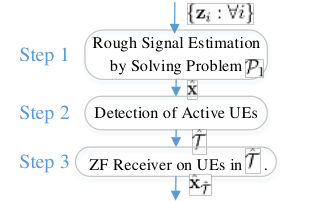
The proposed signal recovery algorithm at the BBU pools consists of three major components: i) rough signal estimation of $\hat{\mathbf{x}}$ using CS techniques; ii) active user detection $\hat{\mathcal{T}}$ based on $\hat{\mathbf{x}}$; and iii) zero-forcing (ZF) receiver based on $\hat{\mathcal{T}}$. Figure 3 illustrates the block diagram of the signal recovery algorithm at the BBU pools. Note that the proposed recovery algorithm is different from the standard CS recovery in [20, 28, 29] because the proposed recovery algorithm has embraced the multi-access fading channel $\{H_{ik}^{[c]}:\forall i,k,c\}$ in the recovery process. The three components are elaborated in detail below.

• •

  Rough signal estimation of $\hat{\mathbf{x}}$ using CS techniques: We first formulate the rough signal estimation of $\hat{\mathbf{x}}$ into a standard CS problem. First, concatenate the compressed symbol vectors $\{\mathbf{z}_{i}\in\mathbb{C}^{R\times 1}:i=1,2,...,M\}$ into a long vector to be $\mathbf{z}=\left[\begin{array}[]{ccc}\mathbf{z}_{1}^{T}&\cdots&\mathbf{z}_{M}^{T}\end{array}\right]^{T}\in\mathbb{C}^{MR\times 1}$. Then, (3) can be equivalently written as

  $$\mathbf{z}=\Theta\mathbf{x}+\mathbf{n},$$

  (7)

  where $\mathbf{n}$ is the aggregate measurement noise

  $$\mathbf{n}=\left[\begin{array}[]{ccc}(\mathbf{A}_{1}\mathbf{n}_{1})^{T}&\cdots&(\mathbf{A}_{M}\mathbf{n}_{M})^{T}\end{array}\right]^{T}\in\mathbb{C}^{MR\times 1},$$

  (8)

  and $\Theta$ is given by (a detailed expression of $\Theta$ is also given in (12))

  $$\Theta=\left[\begin{array}[]{ccc}(\mathbf{A}_{1}\mathbf{H}_{1})^{T}&\cdots&(\mathbf{A}_{M}\mathbf{H}_{M})^{T}\end{array}\right]^{T}\in\mathbb{C}^{MR\times KN_{c}}.$$

  (9)

  Therefore, (7) matches the standard CS model in which $\mathbf{z}$ is the measurements, $\Theta$ is the aggregate measurement matrix, $\mathbf{x}$ is the sparse signal vector to be recovered and $\mathbf{n}$ is the CS measurement noise (with $\mathbb{E}\left(||\mathbf{n}||^{2}\right)=N_{c}$). Note that knowledge of $\Theta$ can be available at the BBU from (9) and the fact that both $\{\mathbf{H}_{i}\}$ and $\{\mathbf{A}_{i}\}$ are available at the BBU. Since the above formulation (7) has incorporated the channel fading of $\{H_{ik}^{[c]}\}$ into the CS measurement model, it enables us to conduct the end-to-end recovery of $\mathbf{x}$. Using the classical basis⁷⁷ 7 Among various CS recovery algorithms [20, 28, 29, 30] (including BP [20], OMP [28], CoSaMP [29] and SP [30]), the BP is shown to has competitive theoretical as well as empirical recovery performance [20], and it does not require the knowledge of the sparsity level (i.e., $\#|\mathcal{T}|$). Therefore, in this paper, we adopt the BP approach to conduct the rough estimation of $\hat{\mathbf{x}}$ in Step 1. pursuit (BP) [20] CS recovery technique, the rough signal recovery of $\hat{\mathbf{x}}$ can be formulated as

  	$\displaystyle\mathcal{P}_{1}:\qquad\min_{\hat{\mathbf{x}}}$		$\displaystyle\left\|\hat{\mathbf{x}}\right\|_{1}$
  	s.t.		$\displaystyle\left\|\Theta\hat{\mathbf{x}}-\mathbf{z}\right\|\leq\lambda.$		(10)

  where $\lambda$ is a proper threshold parameter.

• •

  Active user detection $\hat{\mathcal{T}}$ based on $\hat{\mathbf{x}}$: The following criterion is proposed to detect the set of active UEs $\hat{\mathcal{T}}$:

  	$\displaystyle\hat{\mathcal{T}}$	$\displaystyle=$	$\displaystyle\arg\min_{\hat{\mathcal{T}}}\#|\hat{\mathcal{T}}|,$		(11)
  			$\displaystyle\mbox{s.t.}\begin{cases}|\mathbf{\hat{x}}(i)|\geq|\mathbf{\hat{x}}(j)|,\;\forall i\in\hat{\mathcal{T}},\hskip 9.24994ptj\notin\mathcal{T},\\ \left\|\left(\mathbf{I}-\Theta_{\hat{\mathcal{T}}}\Theta_{\hat{\mathcal{T}}}^{\dagger}\right)\mathbf{z}\right\|\leq\lambda\;\mbox{OR}\;\#|\hat{\mathcal{T}}|=MR.\end{cases}$

  where $\Theta_{\hat{\mathcal{T}}}^{\dagger}\triangleq(\Theta_{\hat{\mathcal{T}}}^{H}\Theta_{\hat{\mathcal{T}}})^{-1}\Theta_{\hat{\mathcal{T}}}^{H}$ denotes the Moore-Penrose pseudoinverse of $\Theta_{\mathcal{\hat{T}}}$.

• •

  Zero-forcing (ZF) receiver based on $\hat{\mathcal{T}}$: The BBU pools apply the zero-forcing receiver $\mathbf{U}=(\Theta_{\mathcal{\hat{T}}}^{\dagger})^{H}$ [31] to recover the transmitted signals from the UEs in $\hat{\mathcal{T}}$, i.e., $\hat{\mathbf{x}}_{\hat{\mathcal{T}}}=\Theta_{\mathcal{T}}^{\dagger}\mathbf{z}$, $\hat{\mathbf{x}}_{\{1,..,KN_{c}\}\backslash\hat{\mathcal{T}}}=\mathbf{0}$.

The overall signal recovery at the BBU pools is summarized in Algorithm 2 (as well as in Figure 3).

Algorithm 2 (Joint Signal Recovery in Uplink C-RAN Systems with CS Techniques)

• •

  Step 1 (Rough Signal Estimation Using BP): Solve Problem $\mathcal{P}_{1}$ to obtain $\hat{\mathbf{x}}$.

• •

  Step 2 (Active User Detection): Find the solution $\hat{\mathcal{T}}$ to (11) via the following steps: First sort $\{|\mathbf{\hat{x}}(i)|:i=1,..,KN_{c}\}$ in descending order to obtain the sorted indices $\{i_{1},i_{2},..,i_{KN_{c}}\}$, initialize $k=1$ and $\hat{\mathcal{T}}=\{i_{1}\}$ and then execute the following to find $\hat{\mathcal{T}}$.

  • –

    (Greedy Detection):If $\left\|\left(\mathbf{I}-\Theta_{\hat{\mathcal{T}}}\Theta_{\hat{\mathcal{T}}}^{\dagger}\right)\mathbf{z}\right\|\leq\lambda$ or⁸⁸ 8 Note that we have constrained the maximum size of $\hat{\mathcal{T}}$ to be $MR$ as in (11). This is because we have a total of $MR$ observations at the BBU so that we can recover $MR$ unknowns at most. $k=MR$, then stop and output $\hat{\mathcal{T}}$. Else, update $k=k+1$, $\hat{\mathcal{T}}=\hat{\mathcal{T}}\bigcup\{i_{k}\}$ and repeat.

• •

  Step 3 (Zero-forcing Receiver): Based on the estimated set of UEs $\hat{\mathcal{T}}$, apply the linear zero-forcing receiver $\mathbf{U}=(\Theta_{\mathcal{\hat{T}}}^{\dagger})^{H}$ [31] to recover the transmitted signals from the UEs in $\hat{\mathcal{T}}$, i.e., $\hat{\mathbf{x}}_{\hat{\mathcal{T}}}=(\Theta_{\mathcal{\hat{T}}}^{\dagger})\mathbf{z}$, $\hat{\mathbf{x}}_{\{1,..,KN_{c}\}\backslash\hat{\mathcal{T}}}=\mathbf{0}$.

Note that when the detected set of active UEs in Algorithm 2 is correct, i.e., $\hat{\mathcal{T}}=\mathcal{T}$, Step 3 in Algorithm 2 will be reduced to classical ZF on the set of the active uplink UEs $\mathcal{T}$ directly. This is the desired performance and it is also asymptotically optimal because of the asymptotical optimality of ZF in high SNR [31]. Under correct active user detection, further analysis [31] on ZF can also be conducted to give further characterization of the C-RAN communication performance (e.g., sum capacity, which will be discussed in Section IV). Therefore, it is critical to first understand the performance of active user detection in Algorithm 2.

Challenge 2: Analyze the probability of correct active user detection, i.e., $\hat{\mathcal{T}}=\mathcal{T}$ in Algorithm 2.

In Algorithm 2, the rough estimation of $\hat{\mathbf{x}}$ in Step 1 plays an important role in the detection of active user $\hat{\mathcal{T}}$ in Step 2. As such, we shall first characterize Step 1 in Algorithm 2 (the BP in Problem $\mathcal{P}_{1}$). In the literature, RIP [20] is commonly adopted to facilitate the performance analysis of the BP. We first review the notion of the RIP in Definition 2 and the associated performance result of BP under RIP in Lemma 1.

Denote event $\mathcal{\mathcal{E}}_{k,\delta}$ as follows:

From [20], we have the following lemma on the recovery performance regarding problem $\mathcal{P}_{1}$.

Based on Lemma 1, we obtain the following conditions for correct active user detection and the associated performance result in Algorithm 2.

In this section, we justify that the RIP condition can be satisfied for our aggregate measurement matrix $\Theta$ (i.e., $\mathcal{\mathcal{E}}_{2s,\delta}$ can happen). Note that not all matrices can satisfy the RIP condition and justifying the RIP of a random matrix is also highly challenging in general [21]. For instance, to prove the RIP property for conventional i.i.d. sub-Gaussian random matrices, the tools of concentration inequalities are needed and lots of math derivations are usually involved to characterize the tail probabilities of sub-Gaussian vectors [33]. On the other hand, the characterization of the RIP for the random matrix $\Theta$ in (12) will be more complicated as $\Theta$ contains a very complicated structure. Specifically, the randomness of $\Theta$ comes from both the block diagonal fading matrices $\{\mathbf{H}_{i}\}$ and the distributed compression matrices $\{\mathbf{A}_{i}\}$. From the expression of $\Theta$ in (12), we have the following two observations:

• •

  Observation I: The columns of $\Theta$ are correlated due to the shared random factors of $\{\mathbf{A}_{i}(r,c)\}$.

• •

  Observation II: The rows of $\Theta$ are correlated due to the shared random factors of $\{\mathbf{H}_{i}\}$.

As such, conventional techniques [33] for characterizing the RIP for i.i.d. sub-Gaussian random matrices cannot be applied to our scenario. In the literature, there are a few works of RIP characterization on structured measurement matrices, such as the Random Demodulator matrix in [34], the Toeplitz matrix in [35], and the random Gaussian matrix with i.i.d. row vectors while having correlated entries within each row [36]. However, these works [34, 35, 36] cannot be used in our scenario due to the different structure of $\Theta$ as described above.

Challenge 3: Analyze the RIP of $\Theta$ despite the complicated structures in the random matrix $\Theta$ in (12).

In the following, we shall establish the RIP condition for $\Theta$. Despite of the complicated structures above, one important feature of $\Theta$ is that under a given realization of $\{\mathbf{H}_{i}\}$, different columns of $\Theta$ are conditionally independent. On the other hand, R. Vershynin et al. shows in [37] that random sub-Gaussian matrices with independent columns is likely to satisfy the RIP with high probability under certain mild conditions. This result [37] enables us to first deploy the conditional probability theory to decompose the proof of RIP of $\Theta$ into several concentration inequalities. We then manage to prove each of these concentration inequalities by following the derivation techniques in [34] and [37]. Specifically, we show that when the number of measurements $R$ at each RRH scales in the order of $\mathcal{O}\left(\frac{s\log^{6}KN_{c}}{M}\right)$, the aggregate measurement matrix $\Theta$ (with special structures) can satisfy the RIP with high probability.

References

- [1] A. Tolli, M. Codreanu, and M. Juntti, “Cooperative MIMO-OFDM cellular system with soft handover between distributed base station antennas,” IEEE Trans. Wireless Commun., vol. 7, no. 4, pp. 1428–1440, 2008.
- [2] C.-X. Wang, X. Hong, X. Ge, X. Cheng, G. Zhang, and J. Thompson, “Cooperative MIMO channel models: a survey,” IEEE Commun. Mag., vol. 48, no. 2, pp. 80–87, 2010.
- [3] C. Mobile, “C-RAN: the road towards green RAN,” White Paper, ver, vol. 2, 2011.
- [4] P. Chanclou, A. Pizzinat, F. Le Clech, T.-L. Reedeker, Y. Lagadec, F. Saliou, B. Le Guyader, L. Guillo, Q. Deniel, S. Gosselin et al., “Optical fiber solution for mobile fronthaul to achieve cloud radio access network,” in Future Network and Mobile Summit (FutureNetworkSummit), 2013. IEEE, 2013, pp. 1–11.
- [5] C. J. Bernardos, A. De Domenico, J. Ortin, P. Rost, and D. Wubben, “Challenges of designing jointly the backhaul and radio access network in a cloud-based mobile network,” in Future Network and Mobile Summit (FutureNetworkSummit), 2013. IEEE, 2013, pp. 1–10.
- [6] C. T. Ng and H. Huang, “Linear precoding in cooperative MIMO cellular networks with limited coordination clusters,” IEEE J. Sel. Areas Commun., vol. 28, no. 9, pp. 1446–1454, 2010.
- [7] M. Hong, R. Sun, H. Baligh, and Z.-Q. Luo, “Joint base station clustering and beamformer design for partial coordinated transmission in heterogeneous networks,” IEEE J. Sel. Areas Commun., vol. 31, no. 2, pp. 226–240, Feb. 2013.
- [8] Y. Zhou and W. Yu, “Optimized backhaul compression for uplink cloud radio access network,” IEEE J. Sel. Areas Commun., vol. 32, no. 6, pp. 1295–1307, June 2014.
- [9] S.-H. Park, O. Simeone, O. Sahin, and S. Shamai, “Robust layered transmission and compression for distributed uplink reception in cloud radio access networks,” IEEE Trans. Veh. Technol., vol. 63, no. 1, pp. 204–216, Jan. 2014.
- [10] ——, “Robust and efficient distributed compression for cloud radio access networks,” IEEE Trans. Veh. Technol., vol. 62, no. 2, pp. 692–703, 2013.
- [11] A. Del Coso and S. Simoens, “Distributed compression for MIMO coordinated networks with a backhaul constraint,” IEEE Trans. Wireless Commun., vol. 8, no. 9, pp. 4698–4709, 2009.
- [12] M. Yun, Y. Rong, Y. Zhou, H.-A. Choi, J.-H. Kim, J. Sohn, and H.-I. Choi, “Analysis of uplink traffic characteristics and impact on performance in mobile data networks,” in Proc. IEEE Int. Conf. Commun. (ICC). IEEE, 2008, pp. 4564–4568.
- [13] V. 3GPP TS 22.368, “Service requirements for machine-type communications,” 3GPP ETSI, Tech. Rep., June 2012. [Online]. Available: http://www.3gpp.org/DynaReport/36211.htm
- [14] M. Hasan, E. Hossain, and D. Niyato, “Random access for machine-to-machine communication in LTE-advanced networks: issues and approaches.” IEEE Commun. Mag., vol. 51, no. 6, 2013.
- [15] A. Laya, L. Alonso, and J. Alonso-Zarate, “Is the random access channel of LTE and LTE-A suitable for M2M communications? A survey of alternatives,” IEEE Commun. Surveys & Tutorials, vol. 16, no. 1, pp. 4–16, First 2014.
- [16] H. Zhu and G. Giannakis, “Sparsity-embracing multiuser detection for CDMA systems with low activity factory,” in Proc. IEEE Int. Symp. Information Theory (ISIT), July 2009, pp. 164–168.
- [17] H. F. Schepker and A. Dekorsy, “Sparse multi-user detection for CDMA transmission using greedy algorithms,” in Proc. IEEE Int. Symp. Wireless Commun. Systems (ISWCS). IEEE, 2011, pp. 291–295.
- [18] H. Zhu and G. B. Giannakis, “Exploiting sparse user activity in multiuser detection,” IEEE Trans. Commun., vol. 59, no. 2, pp. 454–465, 2011.
- [19] D. Baron, M. F. Duarte, M. B. Wakin, S. Sarvotham, and R. G. Baraniuk, “Distributed compressive sensing,” arXiv preprint arXiv:0901.3403, 2005. [Online]. Available: http://arxiv.org/abs/0901.3403
- [20] E. Candes and T. Tao, “Decoding by linear programming,” IEEE Trans. Inf. Theory, vol. 51, no. 12, pp. 4203–4215, 2005.
- [21] E. J. Candès and M. B. Wakin, “An introduction to compressive sampling,” IEEE Signal Process. Mag., vol. 25, no. 2, pp. 21–30, 2008.
- [22] Y. Wang, A. Pandharipande, Y. L. Polo, and G. Leus, “Distributed compressive wide-band spectrum sensing,” in Proc. Inf. Theory and Applications Workshop. IEEE, 2009, pp. 178–183.
- [23] R. 3GPP TS 36.211, “Evolved universal terrestrial radio access (E-UTRA); physical channels and modulation,” 3GPP ETSI, Tech. Rep., 2010. [Online]. Available: http://www.3gpp.org/DynaReport/36211.htm
- [24] Y. Wu, G. Min, K. Li, and B. Javadi, “Modeling and analysis of communication networks in multicluster systems under spatio-temporal bursty traffic,” IEEE Trans. Parallel and Distributed Systems, vol. 23, no. 5, pp. 902–912, 2012.
- [25] H. Huang, S. Misra, W. Tang, H. Barani, and H. Al-Azzawi, “Applications of compressed sensing in communications networks,” arXiv preprint arXiv:1305.3002, 2013. [Online]. Available: http://arxiv.org/abs/1305.3002
- [26] P. Zador, “Asymptotic quantization error of continuous signals and the quantization dimension,” vol. 28, no. 2, pp. 139–149, 1982.
- [27] W. Dai and O. Milenkovic, “Information theoretical and algorithmic approaches to quantized compressive sensing,” IEEE Trans. Commun., vol. 59, no. 7, pp. 1857–1866, 2011.
- [28] J. A. Tropp and A. C. Gilbert, “Signal recovery from random measurements via orthogonal matching pursuit,” IEEE Trans. Inf. Theory, vol. 53, no. 12, pp. 4655–4666, 2007.
- [29] D. Needell and J. A. Tropp, “CoSaMP: Iterative signal recovery from incomplete and inaccurate samples,” Applied and Computational Harmonic Analysis, vol. 26, no. 3, pp. 301–321, 2009.
- [30] W. Dai and O. Milenkovic, “Subspace pursuit for compressive sensing signal reconstruction,” IEEE Trans. Inf. Theory, vol. 55, no. 5, pp. 2230–2249, 2009.
- [31] Y. Jiang, M. K. Varanasi, and J. Li, “Performance analysis of ZF and MMSE equalizers for MIMO systems: an in-depth study of the high snr regime,” IEEE Trans. Inf. Theory, vol. 57, no. 4, pp. 2008–2026, 2011.
- [32] S. Boucheron, G. Lugosi, and O. Bousquet, “Concentration inequalities,” in Advanced Lectures on Machine Learning. Springer, 2004, pp. 208–240.
- [33] R. Baraniuk, M. Davenport, R. DeVore, and M. Wakin, “A simple proof of the restricted isometry property for random matrices,” Constructive Approximation, vol. 28, no. 3, pp. 253–263, 2008.
- [34] J. Tropp, J. Laska, M. Duarte, J. Romberg, and R. Baraniuk, “Beyond nyquist: Efficient sampling of sparse bandlimited signals,” IEEE Trans. Inf. Theory, vol. 56, no. 1, pp. 520–544, Jan. 2010.
- [35] J. Haupt, W. U. Bajwa, G. Raz, and R. Nowak, “Toeplitz compressed sensing matrices with applications to sparse channel estimation,” IEEE Trans. Inf. Theory, vol. 56, no. 11, pp. 5862–5875, 2010.
- [36] G. Raskutti, M. J. Wainwright, and B. Yu, “Restricted eigenvalue properties for correlated gaussian designs,” The Journal of Machine Learning Research, vol. 11, pp. 2241–2259, 2010.
- [37] R. Vershynin, “Introduction to the non-asymptotic analysis of random matrices,” arXiv preprint arXiv:1011.3027, 2010. [Online]. Available: http://arxiv.org/abs/1011.3027
- [38] P. Bartlett, Theoretical Statistics, Lecture 3. UC Berkeley. [Online]. Available: http://www.stat.berkeley.edu/~bartlett/courses/2013spring-stat210b/notes/3notes.pdf
- [39] N. Vakhania, V. Tarieladze, and S. Chobanyan, Probability distributions on Banach spaces. Springer, 1987, vol. 14.