Aspects of gluon propagation in Landau gauge:
spectral densities, and mass scales at finite temperatureThanks: Presented at the “Workshop on Unquenched Hadron Spectroscopy:
Non-Perturbative Models and Methods of QCD vs. Experiment”, at the occasion of Eef van Beveren’s 70th birthday, 1-5 September 2014, University of Coimbra, Portugal

In general, an Euclidean momentum-space propagator $\mathcal{G}(p^{2})\equiv\braket{\mathcal{O}(p)\mathcal{O}(-p)}$ of a (scalar) physical degree of freedom ought to have a Källén-Lehmann spectral representation

The knowledge of the spectral function $\rho(\mu)$ is useful for, amongst other things, to get the masses of the physical states described by the operator $\mathcal{O}$.

Here we describe a method to compute the spectral density given a numerical estimate of the propagator, computed using e.g. lattice techniques. Note that eq. (1) is equivalent to a double Laplace transform $\mathcal{G}=\mathcal{L}^{2}\hat{\rho}=\mathcal{L}\mathcal{L}^{\ast}\hat{\rho}$ where $(\mathcal{L}f)(t)\equiv\int_{0}^{\infty}\mathrm{d}se^{-st}f(s)$; the (double) inversion is then a notorious ill-posed problem, due to the exponential dampening.

For positive spectral functions, a popular approach is the maximum entropy method [1]. An alternative approach, aiming to compute spectral densities not necessarily positive, has been developed by some of us [2], based on the Tikhonov regularization supplemented with the Morozov discrepancy principle.

Specifically, setting $D_{i}\equiv D(p_{i}^{2})$ and assuming we have $N$ data points, we minimize

where we use lattice data in momentum space for the gluon propagator computed in a $80^{4}$ volume, with $\beta=6.0$ (Wilson gauge action) [3]. In eq. (2), $\lambda>0$ is a regularization parameter designed to overcome the ill-posed nature of the inversion. We choose $\lambda$ by means of the Morozov principle: the optimal value $\overline{\lambda}$ is such that the quality of the inversion is equal to the error on the data, i.e. $||D^{reconstructed}-D^{data}||=\delta$ where $\delta$ is the total noise on the input data. The IR regulator (threshold) $\mu_{0}$ will be determined self-consistently by means of the optimal (Morozov) regulator $\overline{\lambda}$: we take the minimal value for $\overline{\lambda}(\mu_{0})$ that can be reached by varying $\mu_{0}$.

The minimization of (2) proceeds through a linear perturbation of $\rho$ and imposing the vanishing of the variation of $\mathcal{J}_{\lambda}$,

The Källén-Lehmann inverse can be computed explicitly

where $\theta(\cdot)$ is the Heaviside step function. We get a linear system for the coefficients $c_{i}$:

with

In Figure 1 we plot the spectral density and, as a check, the reconstructed propagator which can be easily computed combining eqs. (4) and (1). In this case, we have two minima for $\overline{\lambda}(\mu_{0})$, at $\mu_{0}\approx 0.03\penalty\ \textrm{GeV}^{2}$ and $\mu_{0}\approx 0.16\penalty\ \textrm{GeV}^{2}$. We display the results for both values. We conclude that the gluon spectral density is indeed a nonpositive quantity. This is not surprising, since the gluons are not part of the physical spectrum [4]. In the near future, we plan to apply this method to glueballs¹¹ 1 See [5] for a preliminary study of glueball spectral densities. and other physical degrees of freedom.

In this section we briefly describe a recent investigation by some of us [6], where we address the interpretation of the Landau gauge gluon propagator at finite temperature as a massive-type bosonic propagator. For such a goal, we consider a Yukawa-type propagator

where $m$ is the gluon mass and $Z^{\frac{1}{2}}$ the overlap between the gluon state and the quasi-particle massive state.

At finite temperature, the Landau gauge gluon propagator is splitted into two components

where $D_{T}$ and $D_{L}$ are the transverse and longitudinal propagators respectively.

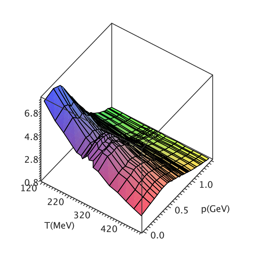
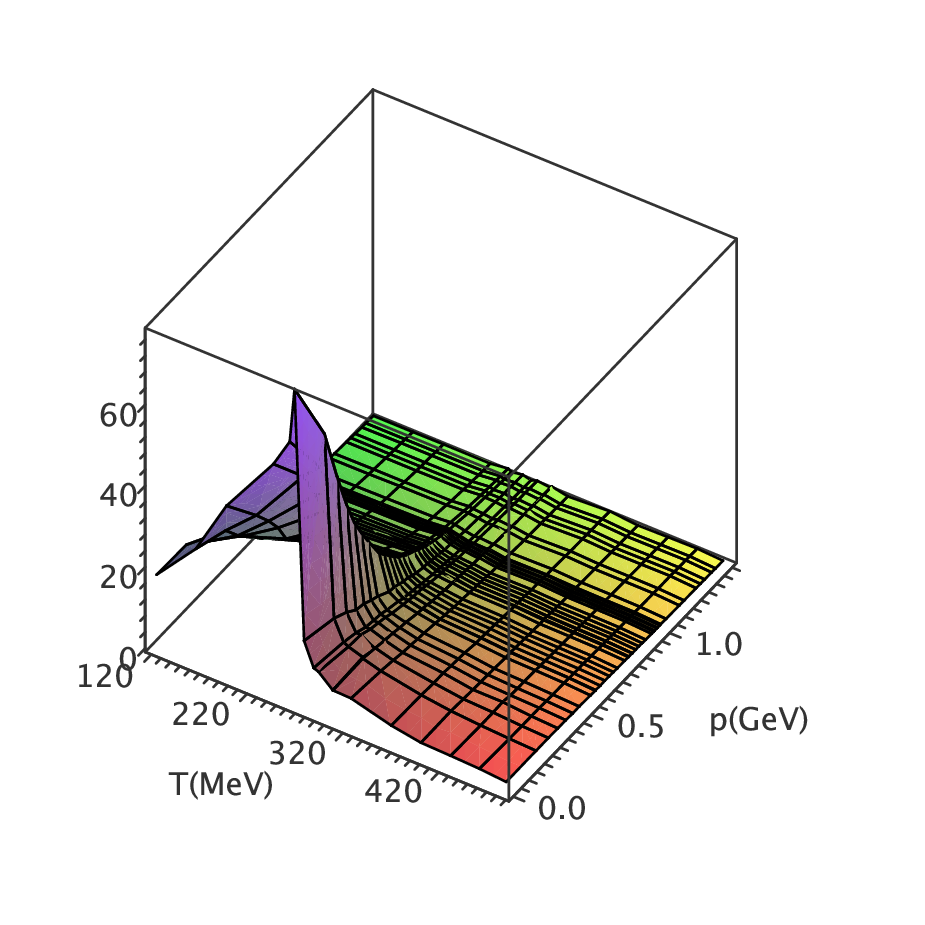
The lattice setup for the simulations at finite temperature considered here is described in Table 1. The surface plots of the two form factors can be seen in Figure 2. For further details see [6].

A simple definition for a mass scale associated with the gluon propagator can be given by

Our results for such a mass scale are shown in Figure 3.

A more realistic value for the gluon mass can be obtained by a fit to the lattice data in the infrared region using the anzatz described in eq. (7). It turns out that the transverse form factor is not described by a Yukawa-type propagator. Therefore one concludes that $D_{T}$ does not behave as quasi-particle massive boson for $T<500$ MeV. In what concerns the longitudinal form factor, we report the values of $Z(T)$ and $m_{g}(T)$ in Figure 4.

We observe that both $m_{g}(T)$ and $Z(T)$ are sensitive to the confinement-deconfinement phase transition; the data suggests that the phase transition is of first order. Below $T_{c}$, the gluon mass is a decreasing function of T, whereas it increases for $T>T_{c}$. Furthermore, the gluon mass follows the expected perturbative behaviour for $T>400$MeV.

Work supported by FCT via projects PTDC/FIS/100968/2008, CERN/ FP/123612/2011, and CERN/FP/123620/2011 developed under the initiative QREN financed by the UE/FEDER through the Programme COMPETE - Programa Operacional Factores de Competitividade. P. J. Silva supported by FCT grant SFRH/BPD/40998/2007. D. Dudal acknowledges financial support from the Research-Foundation Flanders (FWO Vlaanderen) via the Odysseus grant of F. Verstraete. Nuno Cardoso supported by NSF award PHY-1212270.

References

- [1] M. Asakawa, T. Hatsuda and Y. Nakahara, Prog. Part. Nucl. Phys. 46 (2001) 459.
- [2] D. Dudal, O. Oliveira and P. J. Silva, Phys.Rev. D 89 (2014) 014010, arXiv:1310.4069 [hep-lat].
- [3] O. Oliveira and P. J. Silva, Phys. Rev. D 86 (2012) 114513, arXiv:1207.3029 [hep-lat].
- [4] J. M. Cornwall, Mod. Phys. Lett. A 28 (2013) 1330035, arXiv:1310.7897 [hep-ph].
- [5] O. Oliveira, D. Dudal, P. J. Silva, PoS(Lattice 2012)214, arXiv:1210.7794 [hep-lat].
- [6] P. J. Silva, O. Oliveira, P. Bicudo and N. Cardoso, Phys.Rev. D 89 (2014) 074503, arXiv:1310.5629 [hep-lat].
- [7] R. G. Edwards and B. Joó, Nucl.Phys.Proc.Suppl. 140 (2005) 832, arXiv:hep-lat/0409003.
- [8] M. Pippig, SIAM J. Sci. Comput. 35, C213 (2013).