On the complexity of computing MP
distance between binary phylogenetic trees

Steven Kelk Address: Department of Knowledge Engineering (DKE)
Maastricht University
P.O. Box 616, 6200 MD Maastricht
The Netherlands Email: steven.kelk@maastrichtuniversity.nl and Mareike Fischer Address: Ernst-Moritz-Arndt University of Greifswald
Department for Mathematics and Computer Science
Walther-Rathenau-Str. 47
17487 Greifswald, Germany Email: email@mareikefischer.de

Date: August 24, 2026

Abstract.

Within the field of phylogenetics there is great interest in distance measures to quantify the dissimilarity of two trees. Recently, a new distance measure has been proposed: the Maximum Parsimony (MP) distance. This is based on the difference of the parsimony scores of a single character on both trees under consideration, and the goal is to find the character which maximizes this difference. Here we show that computation of MP distance on two binary phylogenetic trees is NP-hard. This is a highly nontrivial extension of an earlier NP-hardness proof for two multifurcating phylogenetic trees, and it is particularly relevant given the prominence of binary trees in the phylogenetics literature. As a corollary to the main hardness result we show that computation of MP distance is also hard on binary trees if the number of states available is bounded. In fact, via a different reduction we show that it is hard even if only two states are available. Finally, as a first response to this hardness we give a simple Integer Linear Program (ILP) formulation which is capable of computing the MP distance exactly for small trees (and for larger trees when only a small number of character states are available) and which is used to computationally verify several auxiliary results required by the hardness proofs.

Key words and phrases:

Maximum Parsimony, phylogenetics, tree metrics, NP-hard, binary trees

1991 Mathematics Subject Classification

05C15; 05C35; 90C35; 92D15

1. Introduction

When present day species are considered and their evolutionary relationships are to be investigated, phylogeneticists often seek to estimate the best evolutionary tree explaining the given species data (e.g. DNA alignments). However, it is well known that different data sets on the same species can lead to different trees, or that different phylogenetic tree estimation methods, like e.g. Maximum Parsimony or Maximum Likelihood or distance based methods, can lead to different trees even for the same data set [10, 6]. Thus, in practice one is often confronted with multiple trees, and it is therefore interesting to measure how different these trees really are. A new way of determining their relative similarity has recently been proposed [5]: the Maximum Parsimony distance (or MP distance, for short).

This metric basically requires the search for a character which has a low parsimony score on one of the trees involved and a high score on the other one. In [5] it has been shown that calculating the MP distance between two trees is NP-hard. The proof presented there required non-binary trees (sometimes also called multifurcating trees). This was not entirely satisfactory, for the following reason. In many branches of phylogenetics multifurcating trees are used to model uncertainty about the precise order of branching events [13], in which case the term unresolved is often used instead of multifurcating. Distance measures which interpret multifurcations this way often have the property that the distance decreases, or in the worst case stays the same, if one or both of the input trees become more unresolved [11]. However, the parsimony score of a single tree increases (or in the best case stays the same) if its edges are contracted to create multifurcations. This is why algorithms that compute Maximum Parsimony trees usually output binary trees: a non-binary solution can be refined into a binary solution without loss of quality. Given this traditional emphasis on binary trees in the parsimony literature, and the fact that evolutionary events such as mutation or speciation are understood to split a lineage into two parts, not three or more [8], it is logical to explore the complexity of MP distance on binary trees.

In this paper, we answer this question by showing that computing the MP distance between two binary trees is, unfortunately, also NP-hard. This is by no means a simple extension of the hardness proofs in [5]. To prove hardness in the present case we are required to develop a rather elaborate array of novel gadgets and arguments, with a strong graph-theoretical flavour.

Moreover, we show as a corollary to the main theorem that this hardness remains if we restrict the number of character states to four (or more). Note that this covers the most important biological applications, as the DNA and RNA alphabets consist of four character states each, and the protein alphabet consists of 20 states. However, when morphological data is analyzed, binary characters are also often relevant, which is why we consider this case, too. We show that when restricted to two character states, calculating the MP distance is not only also NP-hard, but even APX-hard, which means that there exists a constant $c>1$ such that a polynomial-time $c$ -approximation is impossible unless $P=NP$ .

As a tentative first step towards addressing the NP-hardness of the MP distance, we present a simple Integer Linear Program (ILP) which calculates this distance (both on a bounded number of states as well as in the unbounded case). The ILP is rather “explicit” in the sense that it has a static, constraint-based formulation of Fitch’s algorithm embedded within it. Although faster than naive brute force algorithms, the ILP for an unbounded number of states does not scale well and is limited to trees with approximately 16 taxa. On the other hand, the ILP for binary characters is fast: it can cope with trees with up to 100 taxa in reasonable time. In both cases the ILP is fast enough to verify the MP distance of a number of gadgets used in the hardness proofs. An implementation of this ILP has been made publicly available at http://skelk.sdf-eu.org/mpdistbinary/ [12].

2. Notation

Recall that an unrooted phylogenetic $X$ -tree is a tree ${\mathcal{T}}=(V({\mathcal{T}}),E({\mathcal{T}}))$ on a leaf set $X=\{1,\ldots,n\}\subset V({\mathcal{T}})$ . Such a tree is named binary if it has only vertices of degree 1 (leaves) or 3 (internal vertices). A rooted phylogenetic $X$ -tree additionally has one vertex specified as the root, and such a rooted tree is named binary if the root has degree 2 and all other vertices are of degree 1 (leaves) or 3 (internal vertices). Note that two leaves are said to form a cherry, if they are connected to the same inner node. Moreover, a rooted binary tree on three taxa is also often referred to as a rooted triplet, and a rooted tree with only one cherry is also called a caterpillar tree or caterpillar for short. We often denote trees in the well-known Newick format [4], which uses nested parentheses to group species together according to their degree of relatedness. For instance, the tree $((1,2),(3,4))$ is a tree with two so-called cherries $(1,2)$ and $(3,4)$ and a root between the two.

Furthermore, recall that a character $f$ is a function $f:X\rightarrow{\mathcal{C}}$ for some set ${\mathcal{C}}:=\{c_{1},c_{2},c_{3},\ldots,c_{k}\}$ of $k$ character states ( $k\in{\mathbb{N}}$ ). Often, $k$ is assumed to equal 4 in order for ${\mathcal{C}}$ to represent the DNA alphabet $\{A,C,G,T\}$ , but in the present paper $k$ is not restricted this way but can be any natural number unless stated otherwise. Note that in the special case where $|f(X)|=2$ , we also refer to $f$ as a binary character. In general, when $|f(X)|=r$ , $f$ is called an $r$ -state character. In order to shorten the notation, it is customary to write for instance $f=AACC$ instead of $f(1)=A$ , $f(2)=A$ , $f(3)=C$ and $f(4)=C$ . Note that each $r$ -state character $f$ on taxon set $X$ partitions $X$ into $r$ non-empty and non-overlapping subsets $X_{i}$ , $i=1,\ldots,r$ , where $x_{j},x_{k}\in X_{i}$ if and only if $f(x_{j})=f(x_{k})$ .

Note that in this paper, we refer to a character always with its underlying taxon set partition in mind, i.e. for instance we do not distinguish between $AACC$ , $CCAA$ and $CCGG$ , and so on. Moreover, when there is no ambiguity and when the stated result holds for both rooted and unrooted trees, we often just write ‘tree’ or ‘phylogenetic tree’ when referring to a phylogenetic $X$ -tree.

An extension of a character $f$ to $V({\mathcal{T}})$ is a map $g:V({\mathcal{T}})\rightarrow{\mathcal{C}}$ such that $g(i)=f(i)$ for all $i$ in $X$ . For such an extension $g$ of $f$ , we denote by $l_{g}({\mathcal{T}})$ the number of edges $e=\{u,v\}$ in ${\mathcal{T}}$ on which a substitution occurs, i.e. where $g(u)\neq g(v)$ . Such substitutions are also often referred to as mutations or changes. The parsimony score or parsimony length of a character $f$ on ${\mathcal{T}}$ , denoted by $l_{f}({\mathcal{T}})$ , is obtained by minimizing $l_{g}({\mathcal{T}})$ over all possible extensions $g$ of $f$ . For binary trees ${\mathcal{T}}$ , the parsimony score of a character $f$ can easily be calculated with the Fitch algorithm [7]. Recall that the bottom-up phase of Fitch starts at the labelled leaves and assigns to the unlabeled parent of two nodes the intersection of both children’s label set if it is non-empty, or the union otherwise. The top-down phase then starts at the root with an arbitrary choice of the root states suggested by the bottom-up phase and keeps the current state for the descending nodes whenever this is contained in the label set of these nodes, and takes an arbitrary state out of the label set otherwise.

This paper deals with the so-called parsimony distance $d_{MP}$ as introduced in [5]. This distance is defined as follows: Given two phylogenetic trees ${\mathcal{T}}_{1}$ and ${\mathcal{T}}_{2}$ on the same set $X$ of taxa, the parsimony distance between these trees is defined as

d_{MP}({\mathcal{T}}_{1},{\mathcal{T}}_{2})=\max_{f}|l_{f}({\mathcal{T}}_{1})-l_{f}({\mathcal{T}}_{2})|,

where the maximum is taken over all characters $f$ on $X$ . A character $f$ which maximizes this distance is called an optimal character. Note that, due to the fact that the parsimony score of a tree (for a given character) is not affected by the presence or absence of a root, parsimony distance is also oblivious to whether the input trees are rooted or unrooted.

For some proofs in this paper we need the notion of a maximum agreement forest, which is closely linked to the so-called rooted subtree prune and redraft distance or rSPR distance for short. Recall that, informally, an agreement forest of two rooted phylogenetic trees is a set of subtrees which are identical in both trees and which in total contain all leaves, see, e.g. [2]. A maximum agreement forest is an agreement forest with minimum number of components. A single rSPR move involves moving to a neighboring rooted tree by detaching a branch and re-attaching it elsewhere. The rSPR distance $d_{rSPR}$ is the minimum number of rSPR moves required to transform one rooted tree into another. Maximum agreement forests and rSPR distance are closely linked by the well-known result that, modulo a rooting technicality, an agreement forest of two rooted trees with $m$ components yields a set of $m-1$ rSPR moves which turn the first tree into the second one [2].

3. Preliminaries

The following observation, which we will use extensively and implicitly throughout the article, appeared unchanged in our earlier work [5].

Observation 3.1.

Let $f$ be a character on $X$ and ${\mathcal{T}}$ a tree on $X$ . Let $f^{\prime}$ be any character obtained from $f$ by changing the state of exactly one taxon. Then $l_{f}({\mathcal{T}})-1\leq l_{f^{\prime}}({\mathcal{T}})\leq l_{f}({\mathcal{T}})+1$ i.e. the parsimony score can change by at most one.

Proof.

Suppose $l_{f^{\prime}}({\mathcal{T}})\leq l_{f}({\mathcal{T}})-2$ . Consider any extension of $f^{\prime}$ to the interior nodes of ${\mathcal{T}}$ that achieves $l_{f^{\prime}}({\mathcal{T}})$ mutations. Using the same extension but on $f$ gives at most $l_{f^{\prime}}({\mathcal{T}})+1$ mutations, because only one taxon changed state. So $l_{f}({\mathcal{T}})\leq l_{f^{\prime}}({\mathcal{T}})+1\leq l_{f}({\mathcal{T}})-1$ , which is a contradiction. In the other direction, take any optimal extension of $f$ and apply it to $f$ ’. At most one extra mutation will be created, so $l_{f^{\prime}}({\mathcal{T}})\leq l_{f}({\mathcal{T}})+1$ . ∎

A more general version of the following lemma appeared earlier in [5]. Here we have specialized the lemma and its proof to apply to rooted binary trees, which is the type of trees we will construct in the subsequent hardness reductions.

Lemma 3.2.

Let $f$ be an optimal character for two rooted, binary trees ${\mathcal{T}}_{1}$ and ${\mathcal{T}}_{2}$ i.e. $d_{MP}({\mathcal{T}}_{1},{\mathcal{T}}_{2})=|l_{f}({\mathcal{T}}_{2})-l_{f}({\mathcal{T}}_{1})|.$ Without loss of generality assume $l_{f}({\mathcal{T}}_{1})<l_{f}({\mathcal{T}}_{2})$ . Then we can construct in polynomial time an optimal character $f^{\prime}$ with the following property: $l_{f^{\prime}}({\mathcal{T}}_{1})<l_{f^{\prime}}({\mathcal{T}}_{2})$ and for each vertex $u$ of ${\mathcal{T}}_{1}$ such that both $u$ ’s children are leaves (i.e. they form a cherry), $f^{\prime}$ assigns both children of $u$ the same state.

Proof.

Consider a vertex $u$ of ${\mathcal{T}}_{1}$ such that both of its children are taxa, but such that $f$ assigns the two children different states. We calculate an optimal extension of $f$ to the interior nodes of ${\mathcal{T}}_{1}$ by applying Fitch’s algorithm. Let $s$ be the state allocated to $u$ by the top-down phase of Fitch. Choose the child of $u$ that does not have state $s$ and change its state to $s$ . This yields a new character $f^{*}$ . Clearly, $l_{f^{*}}({\mathcal{T}}_{1})<l_{f}({\mathcal{T}}_{1})$ , simply by using the same extension that Fitch gave. Combining this with Observation 3.1 gives $l_{f^{*}}({\mathcal{T}}_{1})=l_{f}({\mathcal{T}}_{1})-1$ and thus $l_{f^{*}}({\mathcal{T}}_{2})=l_{f}({\mathcal{T}}_{2})-1$ (otherwise $f$ could not have been optimal). Hence, $f^{*}$ is also an optimal character, and $l_{f^{*}}({\mathcal{T}}_{1})<l_{f^{*}}({\mathcal{T}}_{2})$ . This process can be repeated for as long as necessary. Termination in polynomial time is guaranteed because each taxon has its state changed at most once. ∎

Observation 3.3.

Lemma 3.2 also holds for optimal characters under the $d_{MP}^{i}({\mathcal{T}}_{1},{\mathcal{T}}_{2})$ model.

Proof.

The transformation in the proof of Lemma 3.2 does not increase the number of states in the character. ∎

4. MP distance on binary trees is NP-hard

4.1. The symmetry-breaking construction

In the hardness proof in Section 4.2 we will construct two trees ${\mathcal{T}}_{E}$ and ${\mathcal{T}}_{V}$ and a central fact used in the proof of correctness of the reduction is that, for all optimal characters $f$ , $l_{f}({\mathcal{T}}_{E})<l_{f}(T_{V})$ . In this section we show how to construct a gadget to enforce this property. Note that all the trees constructed in this section are binary. (As we demonstrated in [5] constructing such a symmetry-breaking gadget is far easier in the non-binary case).

Refer to caption — Figure 1. The two “asymmetric” trees ${\mathcal{T}}_{a}$ and ${\mathcal{T}}_{b}$ and an optimal character $f_{asym}=GAACCG$ .

Consider the two rooted trees

	$\displaystyle{\mathcal{T}}_{a}=(((((2,3),4),5),6),1)$
	$\displaystyle{\mathcal{T}}_{b}=((((2,6),(3,4)),5),1)$

shown in Figure 1. It can be verified computationally that $d_{MP}({\mathcal{T}}_{a},{\mathcal{T}}_{b})=2$ , achieved for example by character $f_{asym}=GAACCG$ ¹¹ 1 Note that for this specific character there exist optimal extensions in both trees such that the root is allocated state $G$ . with $l_{f}({\mathcal{T}}_{a})=2$ and $l_{f}({\mathcal{T}}_{b})=4$ . Moreover, if $f$ is an optimal character, then $l_{f}({\mathcal{T}}_{a})+2=l_{f}({\mathcal{T}}_{b})$ . Expressed differently: there does not exist any optimal character $f$ for which $l_{f}({\mathcal{T}}_{a})>l_{f}({\mathcal{T}}_{b})$ , so the instance is “asymmetric”. For two trees ${\mathcal{T}}_{1}$ and ${\mathcal{T}}_{2}$ , let

gap({\mathcal{T}}_{1},{\mathcal{T}}_{2})=|\max_{f}(l_{f}({\mathcal{T}}_{2})-l_{f}({\mathcal{T}}_{1}))-\max_{f}(l_{f}({\mathcal{T}}_{1})-l_{f}({\mathcal{T}}_{2}))|

where $f$ ranges over all characters (not just optimal ones). Note that $gap({\mathcal{T}}_{a},{\mathcal{T}}_{b})=1$ because $\max_{f}(l_{f}({\mathcal{T}}_{b})-l_{f}({\mathcal{T}}_{a}))=2$ and $\max_{f}(l_{f}({\mathcal{T}}_{a})-l_{f}({\mathcal{T}}_{b}))=1$ , where e.g. the character $f=AACCAA$ achieves $l_{f}({\mathcal{T}}_{a})-l_{f}({\mathcal{T}}_{b})=2-1=1$ .

We now describe an iterative construction such that, for any desired gap $g$ , we can construct two trees ${\mathcal{T}}_{1}$ and ${\mathcal{T}}_{2}$ , both on $O(g)$ taxa, such that $gap({\mathcal{T}}_{1},{\mathcal{T}}_{2})\geq g$ .

We start with ${\mathcal{T}}_{a}$ and ${\mathcal{T}}_{b}$ . Let ${\mathcal{T}}_{A}$ be the rooted tree on 12 taxa obtained by taking two disjoint copies of ${\mathcal{T}}_{a}$ and joining them together via their roots $\rho_{1},\rho_{2}$ to a newly introduced root $\rho$ . (Here, the copying operation is assumed to introduce new taxon labels to prevent the same taxon occuring twice in the same tree). ${\mathcal{T}}_{B}$ is defined the same way, but with respect to ${\mathcal{T}}_{b}$ .

Claim 4.1.

$gap({\mathcal{T}}_{A},{\mathcal{T}}_{B})\geq 2$ .

Proof.

We will show that $\max_{f}(l_{f}({\mathcal{T}}_{B})-l_{f}({\mathcal{T}}_{A}))\geq 4$ and $\max_{f}(l_{f}({\mathcal{T}}_{A})-l_{f}({\mathcal{T}}_{B}))\leq 2$ , from which the claim will follow. Let $f$ be a character such that $l_{f}({\mathcal{T}}_{a})+2=l_{f}({\mathcal{T}}_{b})$ , i.e. $f$ is an optimal character for ${\mathcal{T}}_{a},{\mathcal{T}}_{b}$ . We extend character $f$ to become character $F$ on ${\mathcal{T}}_{A},{\mathcal{T}}_{B}$ in the natural way i.e. disjoint copies of the same taxon receive the same character state. If we run the bottom-up phase of Fitch’s algorithm on ${\mathcal{T}}_{A}$ and ${\mathcal{T}}_{B}$ , we observe that each copy of ${\mathcal{T}}_{a}$ induces 2 fewer mutations than its corresponding copy of ${\mathcal{T}}_{b}$ . Moreover, the set of states identified (by Fitch’s bottom-up phase) to be possible at $\rho_{1}$ will be equal to the set of states identified to be possible at $\rho_{2}$ , so there will be no mutations incurred in ${\mathcal{T}}_{A}$ on the two edges incident to its root $\rho$ . By the same argument, there will be no mutations incurred in ${\mathcal{T}}_{B}$ on the edges incident to its root. Hence, $l_{F}({\mathcal{T}}_{B})-l_{F}({\mathcal{T}}_{A})\geq 4$ . Showing $\max_{f}(l_{f}({\mathcal{T}}_{A})-l_{f}({\mathcal{T}}_{B}))\leq 2$ is possible analytically but it is technical. We therefore omit the proof, noting however that we have used an exhaustive computational search to verify that (a) $\max_{f}(l_{f}({\mathcal{T}}_{B})-l_{f}({\mathcal{T}}_{A}))=4$ , where the maximum is reached e.g. by $f=ABBCCAACCBBA$ and (b) $\max_{f}(l_{f}({\mathcal{T}}_{A})-l_{f}({\mathcal{T}}_{B}))=2$ , where the maximum is reached e.g. by $f=AABBAAAABBAA$ . Note that our ILP described in Section 6 can also be used to verify the claim. The computational search thus allows us to draw the slightly stronger conclusion that $gap({\mathcal{T}}_{A},{\mathcal{T}}_{B})=2$ . ∎

Let ${\mathcal{T}}^{k}_{A}$ be the rooted tree on $12k$ taxa obtained by arranging $k$ disjoint copies of ${\mathcal{T}}_{A}$ along a caterpillar backbone. That is, ${\mathcal{T}}^{1}_{A}={\mathcal{T}}_{A}$ and for $k>1$ , ${\mathcal{T}}^{k}_{A}$ is obtained by joining ${\mathcal{T}}^{k-1}_{A}$ and ${\mathcal{T}}_{A}$ via a new root. ${\mathcal{T}}^{k}_{B}$ is defined analogously.

Claim 4.2.

$gap({\mathcal{T}}^{2}_{A},{\mathcal{T}}^{2}_{B})\geq 3$ .

Proof.

By extending the character $F$ to ${\mathcal{T}}^{2}_{A},{\mathcal{T}}^{2}_{B}$ in the usual fashion, and using the same Fitch-based argument as in the previous proof, we see that $\max_{f}(l_{f}({\mathcal{T}}^{2}_{B})-l_{f}({\mathcal{T}}^{2}_{A}))\geq 8$ . One the other hand, due to the fact that $\max_{f}(l_{f}({\mathcal{T}}_{A})-l_{f}({\mathcal{T}}_{B}))\leq 2$ , the total number of mutations incurred inside the two copies of ${\mathcal{T}}_{A}$ can in total be at most 4 more than the total number of mutations incurred inside the two copies of ${\mathcal{T}}_{B}$ . In the worst case, ${\mathcal{T}}^{2}_{A}$ can perhaps also suffer a single mutation on the two edges incident to the root, while ${\mathcal{T}}^{2}_{B}$ suffers none, so $\max_{f}(l_{f}({\mathcal{T}}^{2}_{A})-l_{f}({\mathcal{T}}^{2}_{B}))\leq 5$ . The claim follows. ∎

Lemma 4.3.

For $k\geq 1$ , $gap({\mathcal{T}}^{k}_{A},{\mathcal{T}}^{k}_{B})\geq k+1$ .

Proof.

We prove this statement by induction. For $k\in\{1,2\}$ the lemma has already been proved, so assume $k\geq 3$ . By continuing the arguments used in the previous claims, we see that

\max_{f}(l_{f}({\mathcal{T}}^{k}_{B})-l_{f}({\mathcal{T}}^{k}_{A}))\geq\max_{f}(l_{f}({\mathcal{T}}^{k-1}_{B})-l_{f}({\mathcal{T}}^{k-1}_{A}))+\max_{f}(l_{f}({\mathcal{T}}_{B})-l_{f}({\mathcal{T}}_{A}))

and

\max_{f}(l_{f}({\mathcal{T}}^{k}_{A})-l_{f}({\mathcal{T}}^{k}_{B}))\leq\max_{f}(l_{f}({\mathcal{T}}^{k-1}_{A})-l_{f}({\mathcal{T}}^{k-1}_{B}))+\max_{f}(l_{f}({\mathcal{T}}_{A})-l_{f}({\mathcal{T}}_{B}))+1

where the 1 in the second expression accounts for the possibility that in ${\mathcal{T}}^{k}_{A}$ a mutation is incurred on one of the root edges, while no such mutation is incurred in ${\mathcal{T}}^{k}_{B}$ . Combining the above with the fact that $\max_{f}(l_{f}({\mathcal{T}}_{B})-l_{f}({\mathcal{T}}_{A}))=4$ , $\max_{f}(l_{f}({\mathcal{T}}_{A})-l_{f}({\mathcal{T}}_{B}))=2$ , $\max_{f}(l_{f}({\mathcal{T}}^{2}_{B})-l_{f}({\mathcal{T}}^{2}_{A}))\geq 8$ and $\max_{f}(l_{f}({\mathcal{T}}^{2}_{A})-l_{f}({\mathcal{T}}^{2}_{B}))\leq 5$ , we obtain the desired result. ∎

In addition to Lemma 4.3, we actually also need to know a (polynomial-time computable) expression for $d_{MP}({\mathcal{T}}^{k}_{A},{\mathcal{T}}^{k}_{B})$ . Conveniently, we have a closed expression for this.

Lemma 4.4.

For $k\geq 2$ , $d_{MP}({\mathcal{T}}^{k}_{A},{\mathcal{T}}^{k}_{B})=8+4(k-2)=4k$ .

Proof.

From the proof of Lemma 4.3 we know that

d_{MP}({\mathcal{T}}^{k}_{A},{\mathcal{T}}^{k}_{B})=max_{f}(l_{f}({\mathcal{T}}^{k}_{B})-l_{f}({\mathcal{T}}^{k}_{A})).

Due to the recurrence shown in the proof of that lemma we see,

max_{f}(l_{f}({\mathcal{T}}^{k}_{B})-l_{f}({\mathcal{T}}^{k}_{A}))\geq 8+4(k-2)

We will complete the proof by showing $d_{MP}({\mathcal{T}}^{k}_{A},{\mathcal{T}}^{k}_{B})\leq 8+4(k-2)$ . To do this, we exploit the fact (proven in [5]) that $d_{MP}({\mathcal{T}}^{k}_{A},{\mathcal{T}}^{k}_{B})\leq d_{rSPR}({\mathcal{T}}^{k}_{A},{\mathcal{T}}^{k}_{B})$ i.e. MP distance is a lower bound on the well-known rooted subtree prune and regraft (rSPR) distance. In particular, we prove that $d_{rSPR}({\mathcal{T}}^{k}_{A},{\mathcal{T}}^{k}_{B})\leq 8+4(k-2)$ . We do this by showing that ${\mathcal{T}}^{k}_{A},{\mathcal{T}}^{k}_{B}$ permit an agreement forest with at most $8+4(k-2)+1=4k+1$ components. (It is well-known that an agreement forest with $m$ components yields a set of $m-1$ rSPR moves that turn one tree into the other, see [2])²² 2 To utilize this agreement forest formulation of rSPR we should first append a new taxon $\rho$ to the root of both trees. However in this case it is easy to check that the omission of $\rho$ does not harm the analysis.. Now, observe that ${\mathcal{T}}^{k}_{A},{\mathcal{T}}^{k}_{B}$ contains $4+2(k-2)=2k$ copies of the original ${\mathcal{T}}_{a},{\mathcal{T}}_{b}$ trees. Next, observe that an agreement forest for ${\mathcal{T}}_{a},{\mathcal{T}}_{b}$ with 3 components can be obtained by placing taxon $3$ and taxon $6$ each in a singleton component, and $\{1,2,4,5\}$ in the remaining component. To obtain an agreement forest for ${\mathcal{T}}^{k}_{A},{\mathcal{T}}^{k}_{B}$ we put all copies of taxon $3$ and all copies of taxon $6$ in singleton components, yielding $4k$ singleton components. All remaining taxa can be placed in one large component, yielding $4k+1$ components in total. ∎

Finally, we consider the following auxiliary observation, which will be useful later.

Observation 4.5.

For each $k\geq 2$ , there exists an optimal character $f^{k}$ on ${\mathcal{T}}^{k}_{A},{\mathcal{T}}^{k}_{B}$ such that $f^{k}$ has 3 states, and there exist optimal extensions of $f^{k}$ to both trees, such that the roots of ${\mathcal{T}}^{k}_{A},{\mathcal{T}}^{k}_{B}$ both receive the same state.

Proof.

As noted earlier, $f_{asym}=GAACCG$ is an optimal character for ${\mathcal{T}}_{a},{\mathcal{T}}_{b}$ and permits optimal extensions such that the roots of both trees can be assigned state $G$ . We can obtain an optimal character $f^{k}$ on ${\mathcal{T}}^{k}_{A},{\mathcal{T}}^{k}_{B}$ simply by making $2k$ copies of $f_{asym}$ . The optimality of $f^{k}$ follows from the fact that $f_{asym}$ is optimal for ${\mathcal{T}}_{a},{\mathcal{T}}_{b}$ and that Claim 4.1 holds for any optimal character. Given that each copy of ${\mathcal{T}}_{a}$ and ${\mathcal{T}}_{b}$ can have state $G$ allocated to its root, it follows (by continuing the bottom-up phase of Fitch on the remainder of ${\mathcal{T}}^{k}_{A}$ and ${\mathcal{T}}^{k}_{B}$ ) that there exist optimal extensions of $f^{k}$ such that the roots of ${\mathcal{T}}^{k}_{A}$ and ${\mathcal{T}}^{k}_{B}$ are both allocated state $G$ . ∎

4.2. The reduction

In this section we exclusively consider simple undirected graphs. Recall that a graph $G=(V,E)$ is cubic if every vertex has degree exactly 3, in which case $|E|=3|V|/2$ . A proper edge colouring of a graph $G$ is an assignment of colours to the edges such that no two adjacent edges have the same colour, where two edges are adjacent if they have a common endpoint. Let $\chi^{\prime}(G)$ , the chromatic index of $G$ , be the minimum number of colours required to properly colour the edges of $G$ . The classical result of Vizing (see any standard graph-theory text, such as [3]) states that for every graph $G$ , $\Delta(G)\leq\chi^{\prime}(G)\leq\Delta(G)+1$ where $\Delta(G)$ is the maximum degree of a vertex in $G$ . Hence, for cubic $G$ , $\chi^{\prime}(G)\in\{3,4\}$ . Even for cubic graphs it is NP-hard to distinguish between these two possibilities [9].

Theorem 4.6.

Computation of $d_{MP}({\mathcal{T}}_{1},{\mathcal{T}}_{2})$ on binary trees is NP-hard.

Proof.

Let $G=(V,E)$ be a cubic graph where $n=|V|$ . We give a polynomial-time reduction from computation of $\chi^{\prime}(G)$ to computation of $d_{MP}$ , from which NP-hardness will follow. Specifically, we will construct two trees ${\mathcal{T}}_{E}$ and ${\mathcal{T}}_{V}$ such that, for a certain integer $P$ , $d_{MP}({\mathcal{T}}_{E},{\mathcal{T}}_{V})=P$ if and only if $\chi^{\prime}(G)=3$ . In particular, if $\chi^{\prime}(G)=4$ , then $d_{MP}({\mathcal{T}}_{E},{\mathcal{T}}_{V})$ will be $P-1$ (or less). An important difference with Theorem 4.6 of [5] is that here optimal characters $f$ will be engineered to always have the property $l_{f}({\mathcal{T}}_{E})<l_{f}({\mathcal{T}}_{V})$ and not the other way round. Informally, at optimality ${\mathcal{T}}_{E}$ always “wins”.

The high-level idea is that in ${\mathcal{T}}_{E}$ we will choose the colours of the edges of $G$ . In fact, for each edge we will choose three colours, all different, representing the colour of $e$ in three different copies of $G$ . Due to the way we construct the two trees, there will exist optimal characters in which the edge colouring (in each of the three copies of $G$ ) is proper. This is because, the closer an edge colouring is to being proper, the higher the parsimony score induced in ${\mathcal{T}}_{V}$ . Within the space of proper edge colourings, we will show that it is advantageous to use as few colours as possible, because this will give the character a low parsimony score on ${\mathcal{T}}_{E}$ . Leveraging the fact that the colours used for the three copies of each edge are all different, we will derive the conclusion that $d_{MP}$ can reach a certain value $P$ if and only if there is a proper edge colouring that uses only 3 colours i.e. that $\chi^{\prime}(G)=3$ . We will prove the following:

		$\displaystyle\chi^{\prime}(G)=3\Rightarrow d_{MP}({\mathcal{T}}_{E},{\mathcal{T}}_{V})=P$
		$\displaystyle\chi^{\prime}(G)=4\Rightarrow d_{MP}({\mathcal{T}}_{E},{\mathcal{T}}_{V})\leq P-1$

Let $M$ be a large integer, at most polynomially large in $n$ , whose value we will specify later. Letting $k=M$ , construct ${\mathcal{T}}^{k}_{A},{\mathcal{T}}^{k}_{B}$ (as described in the previous section). Relabel $S_{E}={\mathcal{T}}^{k}_{A}$ and $S_{V}={\mathcal{T}}^{k}_{B}$ . By Lemma 4.3, $gap(S_{E},S_{V})\geq M+1$ .

The core ingredients of ${\mathcal{T}}_{E}$ are the subtrees $B$ , $S_{E}$ and ${\mathcal{T}}^{***}$ . We construct $B$ by taking an arbitrary rooted binary tree on $3|V|+|E|$ taxa. By appending an extra taxon $\alpha$ just above its root, we create a new root yielding $3|V|+|E|+1$ taxa in total. Note that since $\alpha$ is not a taxon of $B$ , in the following we refer to $B$ including $\alpha$ or $B$ without $\alpha$ to stress whether or not $\alpha$ is considered together with $B$ or not.

Tree $T^{***}$ is constructed as follows. Fix an arbitrary rooted binary tree $T^{*}$ on $|E|$ leaves, identifying the leaves with elements of $E$ . Replace each leaf $u_{e}$ of $T^{*}$ , where $e\in E$ , with a rooted triplet to obtain $T^{**}$ on $3|E|$ leaves $u_{e,j}$ where $e\in E$ and $j\in\{1,2,3\}$ . Finally, replace each leaf $u_{e,j}$ of $T^{**}$ with a rooted triplet on three taxa $x_{e,j}^{u},x_{e,j}^{v}$ and $x_{e,j}^{edge}$ where $u,v\in V$ are the two endpoints of $e$ . We ensure that $x_{e,j}^{u},x_{e,j}^{v}$ are sibling to each other (i.e. form a cherry). This is $T^{***}$ , which is depicted in Figure 2, and it has thus $9|E|$ taxa.

The basic idea is that each edge $e=\{u,v\}$ occurs $3$ times in total, and each such occurrence consists of a cherry representing $u$ and $v$ , and an extra taxon (“edge” ) sitting just above the cherry.

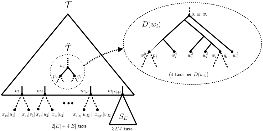
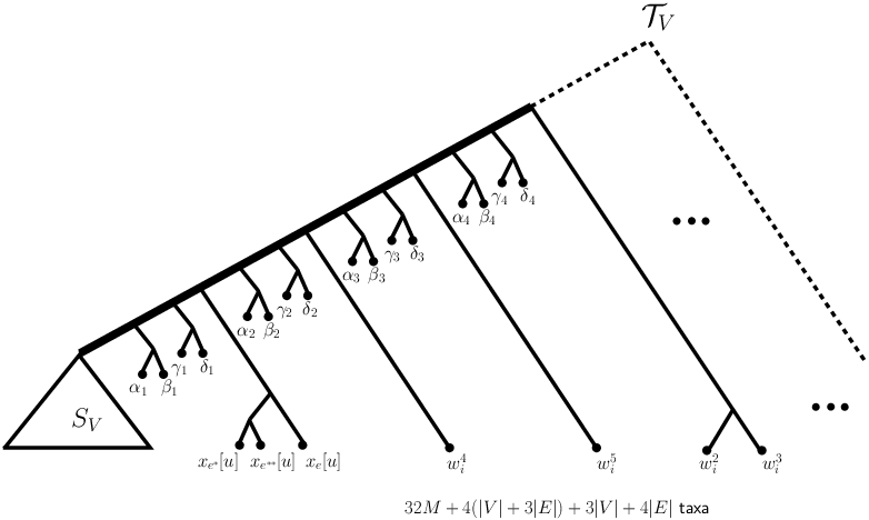
The construction of ${\mathcal{T}}_{E}$ is concluded by joining $B$ including $\alpha$ , $S_{E}$ and $T^{***}$ as shown in Figure 3, which also introduces auxiliary taxa $\beta_{1},\beta_{2},\gamma_{1},\gamma_{2}$ . We adopt the labels used in that figure. Summarizing, ${\mathcal{T}}_{E}$ contains

3|V|+|E|+1+4+9|E|+12M

taxa.

To construct ${\mathcal{T}}_{V}$ we start by taking $B$ and attaching $S_{V}$ on the edge entering taxon $\alpha$ . Now, let

H=\{(v,j)|v\in V,j\in\{1,2,3\}\}\cup\{e|e\in E\}.

Clearly, $|H|=3|V|+|E|$ . Pick an arbitrary bijection between the taxa of $B$ (excluding $\alpha$ ) and the elements of $H$ . For each edge $e\in H$ , introduce a rooted triplet on the three taxa $x_{e,1}^{edge}$ , $x_{e,2}^{edge}$ , $x_{e,3}^{edge}$ and attach this rooted triplet on the edge entering the taxon of $B$ corresponding to $e$ . For each tuple $(v,j)\in H$ , let $\{e,e^{*},e^{**}\}$ be the 3 edges incident to $v$ in $G$ , introduce a rooted triplet on the three taxa $x_{e,j}^{v},x_{e^{*},j}^{v}$ and $x_{e^{**},j}^{v}$ , and attach this rooted triplet on the edge entering the taxon of $B$ corresponding to $(v,j)$ . Finally, we introduce a new root and join $B$ to the new subtree on $((\beta_{1},\gamma_{1}),(\beta_{2},\gamma_{2}))$ . This completes the construction of ${\mathcal{T}}_{V}$ , which is depicted in Figure 4.

We are now in a position to specify the number $M$ . We require $M$ to be sufficiently large that, for every optimal character $f$ , $l_{f}({\mathcal{T}}_{E})<l_{f}({\mathcal{T}}_{V})$ . From Lemma 4.4 we know that there exists some character $f^{\prime}$ such that $l_{f^{\prime}}({\mathcal{T}}_{V})-l_{f^{\prime}}({\mathcal{T}}_{E})\geq 4M$ . (In particular, we can obtain such a character by – for example – extending the character suggested by Lemma 4.4 such that all taxa outside $S_{E}$ and $S_{V}$ are assigned the same state.) Now, let $t$ be the number of edges in ${\mathcal{T}}_{E}$ that lie outside $S_{E}$ . For every character $f$ we have

l_{f}({\mathcal{T}}_{E})-l_{f}({\mathcal{T}}_{V})\leq t+(4M-(M+1)).

The $4M$ term is obtained from Lemma 4.4, the $(M+1)$ term from Lemma 4.3, and the $t$ term arises (pessimistically) from the situation when every edge in ${\mathcal{T}}_{E}$ (outside $S_{E}$ ) incurs a mutation, but no edge in ${\mathcal{T}}_{V}$ (outside $S_{V}$ ) incurs a mutation. So, if we choose $M$ such that

t+4M-(M+1)<4M

it follows that for every optimal character $f$ , $d_{MP}({\mathcal{T}}_{V},{\mathcal{T}}_{E})=l_{f}({\mathcal{T}}_{V})-l_{f}({\mathcal{T}}_{E})$ and in particular $l_{f}({\mathcal{T}}_{V})>l_{f}({\mathcal{T}}_{E})$ . Choosing $M=t$ is therefore sufficient to achieve this. This “symmetry breaking” has far-reaching consequences which we shall heavily utilize later.

Next, let $f^{S}$ be any 3-state character on the taxa in $S_{E}$ and $S_{V}$ such that $l_{f^{S}}({\mathcal{T}}_{V})-l_{f^{S}}({\mathcal{T}}_{E})=4M=d_{MP}(S_{E},S_{V})$ . This character exists and can be constructed in polynomial time thanks to Observation 4.5. Recall, in particular, that it is constructed by making many disjoint copies of the character $f_{asym}=GAACCG$ .

Now, suppose $\chi^{\prime}(G)=3$ . We will extend $f^{S}$ to all the taxa in ${\mathcal{T}}_{E}$ as follows, obtaining a 4-state character. Take any proper edge colouring $Col$ of graph $G$ using three colours red, blue and green. We start by relabelling $f^{S}$ as follows: character state $G$ maps to blue, $A$ maps to red and $C$ maps to green. Next, colour all the taxa in $B$ including $\alpha$ pink. Colour the cherry $\{\beta_{1},\beta_{2}\}$ pink and the cherry $\{\gamma_{1},\gamma_{2}\}$ blue.

Next, consider the following cyclical mapping $F$ :

	$\displaystyle F(red,1)$	$\displaystyle\rightarrow red$
	$\displaystyle F(red,2)$	$\displaystyle\rightarrow blue$
	$\displaystyle F(red,3)$	$\displaystyle\rightarrow green$
	$\displaystyle F(blue,1)$	$\displaystyle\rightarrow blue$
	$\displaystyle F(blue,2)$	$\displaystyle\rightarrow green$
	$\displaystyle F(blue,3)$	$\displaystyle\rightarrow red$
	$\displaystyle F(green,1)$	$\displaystyle\rightarrow green$
	$\displaystyle F(green,2)$	$\displaystyle\rightarrow red$
	$\displaystyle F(green,3)$	$\displaystyle\rightarrow blue$

Now, for every $e\in E$ , $j\in\{1,2,3\}$ and letting $e=\{u,v\}$ , we assign $x_{e,j}^{u},x_{e,j}^{v}$ and $x_{e,j}^{edge}$ all the same colour: the colour $F(Col(e),j)$ where as usual $Col(e)$ is the colour assigned to $e$ by the proper edge colouring $Col$ .

Let this character be called $f^{Col}$ . Observe,

l_{f^{Col}}({\mathcal{T}}_{E})=1+2|E|+l_{f^{S}}(S_{E})

This can be confirmed by applying Fitch’s algorithm. Note, in particular, that there is an optimal extension such that all the internal nodes of the tree $B$ (including $\alpha$ ) are coloured pink, all the nodes of the $T^{*}$ part of $T^{***}$ are blue, $p_{2}$ is blue, the root is blue, and all the unlabelled nodes are blue. The $+1$ is then the mutation in the transition from pink to blue on, for example, the edge between the cherries $\{\beta_{1},\beta_{2}\}$ and $\{\gamma_{1},\gamma_{2}\}$ . There is no mutation on the edge entering the root of $S_{E}$ because, by Observation 4.5 and the way we relabelled $f^{S}$ , there is an optimal extension of $S_{E}$ in which its root is permitted to be blue.

Also,

l_{f^{Col}}({\mathcal{T}}_{V})=2+3(3|V|+|E|)+1+l_{f^{S}}(S_{V})

The $+1$ term here is definitely incurred because there is an optimal extension in which the root of ${\mathcal{T}}_{V}$ and $\alpha$ are both coloured pink, but pink is not used in $f^{S}$ , so there will then be a mutation on the edge entering the root of $S_{V}$ . The $+2$ term corresponds to mutations incurred in the $\beta_{1},\beta_{2},\gamma_{1},\gamma_{2}$ region of ${\mathcal{T}}_{V}$ .

Now, define $P$ as follows:

	$\displaystyle P$	$\displaystyle=l_{f^{Col}}({\mathcal{T}}_{V})-l_{f^{Col}}({\mathcal{T}}_{E})$
		$\displaystyle=\bigg(2+3(3\|V\|+\|E\|)+1+l_{f^{S}}(S_{V})\bigg)-\bigg(1+2\|E\|+l_{f^{S}}(S_{E})\bigg)$
		$\displaystyle=\bigg(2+3(3\|V\|+\|E\|)+1\bigg)-\bigg(1+2\|E\|\bigg)+4M$

Hence, if $\chi^{\prime}(G)=3$ , $d_{MP}({\mathcal{T}}_{E},{\mathcal{T}}_{V})\geq P$ . We still need to show (1) $d_{MP}({\mathcal{T}}_{E},{\mathcal{T}}_{V})\leq P$ and (2) $d_{MP}({\mathcal{T}}_{E},{\mathcal{T}}_{V})=P$ if and only if $\chi^{\prime}(G)=3$ . Once these facts have been established NP-hardness will follow.

We approach this by starting from an arbitrary optimal character $f$ and then transforming $f$ step by step such that we do not lose optimality but the character attains a certain canonical form. This canonical form will be attained by accumulating one special property at a time. In all cases the argument that a new property can be obtained, is based on the assumption that all earlier properties have already been accumulated. Properties are never lost, and each property can be attained in polynomial time. Thus, given an arbitrary optimal character we can transform it in polynomial time into a character that has all the described properties. The proofs of the following properties can be found in the Appendix (unless stated here).

Property 1. All cherries in ${\mathcal{T}}_{E}$ are monochromatic. That is, if $\{x,y\}$ are two taxa that share a parent in ${\mathcal{T}}_{E}$ , then both are assigned the same colour (i.e. state).

Proof. This is possible by combining Lemma 3.2 with the fact (established earlier) that, for every optimal character $f$ , $l_{f}({\mathcal{T}}_{E})<l_{f}({\mathcal{T}}_{V})$ .

Property 2.1. In ${\mathcal{T}}_{E}$ , the cherry $\{\beta_{1},\beta_{2}\}$ has a different colour to the cherry $\{\gamma_{1},\gamma_{2}\}$ .

Property 2.2. In ${\mathcal{T}}_{E}$ , the (possibly multiple) colours used for the taxa of $B$ (including $\alpha$ ) are not used elsewhere in ${\mathcal{T}}_{E}$ , except possibly $\{\beta_{1},\beta_{2}\}$ .

Property 2.3 In ${\mathcal{T}}_{E}$ , all the taxa in $B$ have the same colour which, with the possible exception of $\beta_{1},\beta_{2}$ , does not appear on taxa outside $B$ and $\alpha$ .

Property 3. In ${\mathcal{T}}_{E}$ , all the taxa in $B$ have the same colour, and cherry $\{\beta_{1},\beta_{2}\}$ also has this colour. Moreover this colour does not appear on any other taxa i.e. it is unique for $B$ (including $\alpha$ ) and $\beta_{1},\beta_{2}$ .

From now on we refer to the unique colour used by $B$ (including $\alpha$ ), $\beta_{1}$ and $\beta_{2}$ as pink. Property 3 is extremely important. In particular, it means that from now on we can assume the existence of optimal extensions of ${\mathcal{T}}_{V}$ such that the root of ${\mathcal{T}}_{V}$ is coloured pink and, moreover, that the entire image of $B$ inside ${\mathcal{T}}_{V}$ is coloured pink. We call these pink extensions. These greatly simplifies the task of counting mutations inside ${\mathcal{T}}_{V}$ . In particular, it means that we from now on (in ${\mathcal{T}}_{V}$ ) only need to consider mutations incurred inside the subtrees sibling to the taxa of $B$ , which we call below pink subtrees. These subtrees never contain pink taxa.

Property 4. Let $f$ be an optimal character with properties 1–3 and let $f^{*}$ be the restriction of $f$ to the taxa in $S_{V}$ and $S_{E}$ . Then $l_{f^{*}}(S_{V})-l_{f^{*}}(S_{E})=d_{MP}(S_{E},S_{V})$ .

Proof. Fix a pink extension of $f$ . From the earlier properties, $f^{*}$ does not contain any pink taxa. Now, taxon $\alpha$ is coloured pink, because $\alpha$ is a taxon of $B$ . This means that, in ${\mathcal{T}}_{V}$ , there is unavoidably a mutation on the edge entering the root of $S_{V}$ . Moreover, we know that there exist optimal characters for $S_{E},S_{V}$ in which the roots of $S_{E}$ and $S_{V}$ can be allocated the same colour blue: this is the 3-state character $f^{S}$ that we constructed at the start of the proof. This means that, without loss of optimality, we can assume $f^{*}=f^{S}$ , where we are free to (and should) relabel the blue inside $f^{S}$ such that in ${\mathcal{T}}_{E}$ no mutation is incurred on the edge entering the root of $S_{E}$ . (This can be achieved by running the bottom-up phase of Fitch on the subtree sibling to $S_{E}$ in ${\mathcal{T}}_{E}$ , identifying the set of colours permitted by Fitch at the root of the subtree, and arbitrarily picking one of those colours as the relabelling colour). Optimality is assured because (1) $l_{f^{S}}(S_{V})-l_{f^{S}}(S_{E})=d_{MP}(S_{E},S_{V})$ , (2) we force a mutation at the root of $S_{V}$ and (3) we definitely avoid a mutation at the root of $S_{E}$ .

Property 5. (a) For every edge $e=\{u,v\}\in E$ the three taxa $x_{e,1}^{edge}$ , $x_{e,2}^{edge}$ , $x_{e,3}^{edge}$ all have distinct colours. Moreover, (b) $x_{e,1}^{edge},x_{e,1}^{u},x_{e,1}^{v}$ all have the same colour, $x_{e,2}^{edge},x_{e,2}^{u},x_{e,2}^{v}$ all have the same colour, and finally $x_{e,3}^{edge},x_{e,3}^{u},x_{e,3}^{v}$ all have the same colour.

Proof. First, suppose for some $e\in E$ there exists $j,j^{\prime}\in\{1,2,3\}$ such that $j\neq j^{\prime}$ and $x_{e,j}^{edge}$ , $x_{e,j^{\prime}}^{edge}$ have the same colour. Observe that $x_{e,1}^{edge}$ , $x_{e,2}^{edge}$ , $x_{e,3}^{edge}$ all form a single below pink subtree in ${\mathcal{T}}_{V}$ . Suppose we recolour $x_{e,j}^{edge}$ to some brand new colour. This raises the parsimony score of ${\mathcal{T}}_{E}$ by at most 1. However, it also raises the parsimony score of ${\mathcal{T}}_{V}$ by at least one, due to the introduction of a new colour into the corresponding below pink subtree. Hence the recoloured character is optimal. We can repeat this as long as necessary to ensure that (a) eventually holds. Now, suppose for some $e\in E$ and $j\in\{1,2,3\}$ the taxa $x_{e,j}^{edge},x_{e,j}^{u},x_{e,j}^{v}$ do not all have the same colour. By Property 1 we know that $x_{e,j}^{u}$ and $x_{e,j}^{v}$ have the same colour, because they form a cherry in ${\mathcal{T}}_{E}$ . We recolour all 3 taxa with a brand new colour. This cannot raise the parsimony score of ${\mathcal{T}}_{E}$ . On the other hand, it cannot lower the parsimony score of ${\mathcal{T}}_{V}$ , because the three now uniquely coloured taxa all occur in different below pink subtrees of ${\mathcal{T}}_{V}$ . Hence the recoloured character is optimal, and (a) is still holding. We repeat this as long as necessary to ensure that (b) eventually also holds.

Property 6. For every $j\in\{1,2,3\}$ , the edge colouring induced by the colours of the $x_{e,j}^{edge}$ taxa ( $e\in E$ ), is a proper edge colouring.

Recall that, by Property 5, each $x_{e,j}^{edge}$ taxon has the same colour as the $x_{e,j}^{u}$ and $x_{e,j}^{v}$ taxa below it in ${\mathcal{T}}_{E}$ . Suppose that there is some $j\in\{1,2,3\}$ for which the induced edge colouring is not proper. Then there exists some $u\in V$ and two edges $e\neq e^{\prime}$ in $E$ incident at $u$ such that $x_{e,j}^{u}$ and $x_{e^{\prime},j}^{u}$ both have the same colour. Both these taxa are together in a below pink subtree of ${\mathcal{T}}_{V}$ . This subtree therefore currently induces $m<2$ mutations (excluding the mutation as the subtree touches the pink region). Now, suppose we introduce a brand new colour and recolour $x_{e,j}^{u},x_{e,j}^{v}$ and $x_{e,j}^{edge}$ with it. This raises the parsimony score of ${\mathcal{T}}_{E}$ by at most 1. However, it definitely also raises the parsimony score of ${\mathcal{T}}_{V}$ , by at least 1, because the aforementioned below pink subtree now induces $m+1$ mutations (due to the introduction of a new colour). Hence the new character is optimal, and all earlier properties are preserved. We can repeat this process until the induced edge colouring is proper.

Property 7. For an optimal character $f$ ,

l_{f}({\mathcal{T}}_{V})=2+3(3|V|+|E|)+1+l_{f^{S}}(S_{V}).

Proof. This is a consequence of the fact that (from Property 6) we can assume that in ${\mathcal{T}}_{V}$ a proper edge colouring is induced, plus the fact that a pink extension is an optimal extension. In particular, the proper edge colouring means that each of the $3|V|+|E|$ below pink subtrees induces 2 mutations on its internal edges and a third mutation where the subtree touches the pink region. The ‘2’ term corresponds to the fact that the two taxa $\gamma_{1},\gamma_{2}$ are necessarily not pink. The ’1’ term is the mutation at the root of $S_{V}$ .

Central argument

As a consequence of Property 7, optimal characters (which we always assume to induce proper edge colourings) are only distinguished by their ability to minimize the number of mutations induced in ${\mathcal{T}}_{E}$ . We can already establish a strong lower bound for this number:

l_{f}({\mathcal{T}}_{E})\geq 1+2|E|+l_{f^{S}}(S_{E})

Every proper edge colouring induces (at least) these mutations in ${\mathcal{T}}_{E}$ . The ’1’ term is the mutation that occurs between the $\beta_{1},\beta_{2}$ and $\gamma_{1},\gamma_{2}$ taxa and the $2|E|$ term is a consequence of (amongst others) Property 5.

Hence, $d_{MP}({\mathcal{T}}_{E},{\mathcal{T}}_{V})=l_{f}({\mathcal{T}}_{V})-l_{f}({\mathcal{T}}_{E})\leq P$ , where $P$ is the value defined earlier in the proof. We have already shown that, if $G$ has $\chi^{\prime}(G)=3$ , $P$ is possible. We now see that this is optimal. The only thing we have left to show, is that if $\chi^{\prime}(G)>3$ , that $P$ is not possible. We use the contrapositive to prove this. In particular, we will show

l_{f}({\mathcal{T}}_{E})=1+2|E|+l_{f^{S}}(S_{E})\Rightarrow\chi^{\prime}(G)=3.

Suppose, then, that $l_{f}({\mathcal{T}}_{E})=1+2|E|+l_{f^{S}}(S_{E})$ . This means that there are no mutations in the subtree $T^{***}$ other than the $2|E|$ unavoidable mutations due to Property 5. To achieve this it must be the case that all the $|E|$ subtrees (each containing 9 taxa) in $T^{***}$ all have a single colour in common. Let us call this colour blue. Hence, for every $e\in E$ , there exists exactly one $j\in\{1,2,3\}$ such that $x_{e,j}^{edge},x_{e,j}^{u},x_{e,j}^{v}$ are all blue. We now build a proper 3-edge-colouring for $G$ . If $j=1$ , we assign $e$ the colour red. If $j=2$ , we assign $e$ the colour blue. If $j=3$ , we assign $e$ the colour green. This must be a proper colouring: if it was not, then there would be some vertex $u\in V$ , two incident edges $e,e^{\prime}$ incident to $u$ , and some $j\in\{1,2,3\}$ such that $x_{e,j}^{edge}$ and $x_{e^{\prime},j}^{edge}$ were both blue. But this would contradict Property 6. Hence, $\chi^{\prime}(G)=3$ .

This completes the proof. Summarising, for a given cubic graph $G=(V,E)$ ,

\chi^{\prime}(G)=3\Leftrightarrow d_{MP}({\mathcal{T}}_{E},{\mathcal{T}}_{V})=P,

from which the NP-hardness of computing $d_{MP}({\mathcal{T}}_{E},{\mathcal{T}}_{V})$ on binary trees follows.

∎

Corollary 4.7.

For every fixed integer $i\geq 4$ , computation of $d^{i}_{MP}$ on binary trees is NP-hard.

Proof.

This is a consequence of the fact that in the theorem only 4 states are required to construct a character achieving MP distance $P$ . Namely, the 3 colours used in the proper edge colouring of $G$ , plus pink. ∎

Note that the above proof cannot (obviously) be extended to give APX-hardness. By taking multiple copies of the tree $T^{***}$ it is possible to increase the gap between $\chi^{\prime}(G)=3$ and $\chi^{\prime}(G)=4$ instances to more than 1, but this is insufficient for APX-hardness.

5. Computation of $d^{2}_{MP}$ is NP-hard on binary trees.

As in the previous section we first require a gadget that can break symmetry between two trees.

5.1. Symmetry breaking gadget in the case of 2 states

Consider the two rooted trees

T_{a}=(((5,(6,4)),3),((1,(8,2)),7))

and

T_{b}=(((7,((4,2),6)),3),(8,(1,5)))

shown in Figure 5.

Here, it can be verified (e.g. by exhaustive search) that $d^{2}_{MP}({\mathcal{T}}_{a},{\mathcal{T}}_{b})=3$ , and the character $f_{asym}=AAGGGGAA$ can achieve this: $l_{f_{asym}}({\mathcal{T}}_{a})=1$ and $l_{f_{asym}}({\mathcal{T}}_{b})=4$ .

In fact, these trees are asymmetric, in the sense that for every optimal 2-state character $f$ , $l_{f}({\mathcal{T}}_{a})<l_{f}({\mathcal{T}}_{b})$ . In particular, as can be verified by computational search (e.g. using the ILP formulation or performing an exhaustive search), $\max_{f}(l_{f}({\mathcal{T}}_{b})-l_{f}({\mathcal{T}}_{a}))=3$ and $\max_{f}(l_{f}({\mathcal{T}}_{a})-l_{f}({\mathcal{T}}_{b}))=2$ . (The second maximum is achieved by the character $AAGAAGGG$ , for example.) Using the same notation as in Section 4.1, but restricted to characters with at most 2 states, we therefore obtain:

gap({\mathcal{T}}_{a},{\mathcal{T}}_{b})=1.

From now on we implicitly assume that all characters have at most 2 states.

Define ${\mathcal{T}}_{A}$ and ${\mathcal{T}}_{B}$ in the same way as in Section 4.1. It can be verified that $gap({\mathcal{T}}_{A},{\mathcal{T}}_{B})\geq 1$ . This is not yet strong enough for what we require, so let ${\mathcal{T}}_{AA}$ and ${\mathcal{T}}_{BB}$ be obtained by joining two copies of ${\mathcal{T}}_{A}$ , and two copies of ${\mathcal{T}}_{B}$ , together (respectively).

Claim 5.1.

$gap({\mathcal{T}}_{AA},{\mathcal{T}}_{BB})\geq 2.$

Proof.

It can easily be checked that $\max_{f}(l_{f}({\mathcal{T}}_{BB})-l_{f}({\mathcal{T}}_{AA}))\geq 12$ . This can be achieved, for example, by taking a character $f$ that comprises 4 disjoint copies of $f_{asym}$ , thus obtaining $l_{f}({\mathcal{T}}_{BB})=16$ and $l_{f}({\mathcal{T}}_{AA})=4$ . (In fact, by performing an exhaustive search, one can show that this is optimal). Verifying that $\max_{f}(l_{f}({\mathcal{T}}_{AA})-l_{f}({\mathcal{T}}_{BB}))=10$ is more challenging. We have used an exhaustive search to check this, but note that our ILP gives the same result in significantly less time. In fact, $l_{f}({\mathcal{T}}_{AA})-l_{f}({\mathcal{T}}_{BB})=10$ can be achieved by $f=AGAGAGGAAGGGAGGAGAAAGAAGAGGGAGGA$ , for which the score on ${\mathcal{T}}_{AA}$ is 14 and the score on tree ${\mathcal{T}}_{BB}$ is 4. So, altogether we have $\max_{f}(l_{f}({\mathcal{T}}_{BB})-l_{f}({\mathcal{T}}_{AA}))=12$ and $\max_{f}(l_{f}({\mathcal{T}}_{AA})-l_{f}({\mathcal{T}}_{BB}))=10$ , so $gap({\mathcal{T}}_{AA},{\mathcal{T}}_{BB})\geq 2$ and $d^{2}_{MP}({\mathcal{T}}_{AA},{\mathcal{T}}_{BB})=12$ . ∎

Let ${\mathcal{T}}^{k}_{AA}$ be the rooted tree on $32k$ taxa obtained by arranging $k$ disjoint copies of ${\mathcal{T}}_{AA}$ along a caterpillar backbone. That is, ${\mathcal{T}}^{1}_{AA}={\mathcal{T}}_{AA}$ and for $k>1$ , ${\mathcal{T}}^{k}_{AA}$ is obtained by joining ${\mathcal{T}}^{k-1}_{AA}$ and ${\mathcal{T}}_{AA}$ via a new root. ${\mathcal{T}}^{k}_{BB}$ is defined analogously.

Lemma 5.2.

For $k\geq 1$ , $gap({\mathcal{T}}^{k}_{AA},{\mathcal{T}}^{k}_{BB})\geq k+1$ .

Proof.

The case $k=1$ is proven by Claim 5.1 and for higher $k$ we use analogous arguments to the proof of Claim 4.2 and Lemma 4.3. We omit details. ∎

Lemma 5.3.

For $k\geq 1$ , $d^{2}_{MP}({\mathcal{T}}^{k}_{AA},{\mathcal{T}}^{k}_{BB})=12k$ .

Proof.

${\mathcal{T}}^{k}_{AA}$ comprises $4k$ copies of ${\mathcal{T}}_{a}$ . By taking $4k$ copies of character $f_{asym}$ , we see that $d^{2}_{MP}({\mathcal{T}}^{k}_{AA},{\mathcal{T}}^{k}_{BB})\geq 4k(4-1)=12k$ . That $12k$ is also the upper bound, can be verified by showing $d_{rSPR}({\mathcal{T}}^{k}_{AA},{\mathcal{T}}^{k}_{BB})\leq 12k$ . This follows because by cutting off all copies of taxa $2,5,7$ into separate components, we obtain an agreement forest of ${\mathcal{T}}^{k}_{AA},{\mathcal{T}}^{k}_{BB}$ containing $12k+1$ components. ∎

5.2. The reduction

We reduce from the NP-hard (and APX-hard) problem CUBIC MAX CUT [1]. Here we are given a cubic graph $G=(V,E)$ , $|E|=3|V|/2$ , and we are asked to partition $V$ into two disjoint pieces $V_{1}\cup V_{2}$ such that the number of edges that have one endpoint in $V_{1}$ and one endpoint in $V_{2}$ (“cut” edges), is maximized. Let $MAXCUT(G)$ represent this value. We can assume without loss of generality that $G$ is connected and not bipartite.

The high-level idea is similar to the 2-state hardness reduction in [5]. Namely, we will construct two trees ${\mathcal{T}}_{V}$ and ${\mathcal{T}}_{E}$ and apply the symmetry-breaking gadget to ensure that for all optimal characters $f$ , $l_{f}({\mathcal{T}}_{V})<l_{f}({\mathcal{T}}_{E})$ . We will model the vertices as subtrees in ${\mathcal{T}}_{V}$ , each comprising three taxa, and argue - via a technical argument - that these subtrees are monochromatic. We will let the 2 states represent the two sides of the chosen partition $V_{1}\cup V_{2}$ . Henceforth we will call these states red and blue. The colour of a vertex subtree thus denotes which side of the partition it is on. The tree ${\mathcal{T}}_{E}$ will be constructed such that, the more cut edges are induced by the partition chosen by ${\mathcal{T}}_{V}$ , the higher the parsimony score of ${\mathcal{T}}_{E}$ . The construction will thus naturally choose a character that maximizes $MAXCUT(G)$ .

The fact that ${\mathcal{T}}_{V}$ and ${\mathcal{T}}_{E}$ must be binary, introduces significant complications compared to the 2-state hardness reduction in [5]. For this reason we will introduce two new special gadgets, that allow ${\mathcal{T}}_{V}$ (respectively, ${\mathcal{T}}_{E}$ ) to be viewed as the independent union of several subtrees. In ${\mathcal{T}}_{V}$ the gadget will be called the cherry switch and in ${\mathcal{T}}_{E}$ we will have the $D(w_{i})$ gadget, to be explained in due course. These independence gadgets neutralise the influence of side-effects that can occur as a consequence of the fact that ${\mathcal{T}}_{V}$ and ${\mathcal{T}}_{E}$ are both binary.

We begin by constructing ${\mathcal{T}}_{E}$ . First, we construct the left-hand side subtree ${\mathcal{T}}$ of ${\mathcal{T}}_{E}$ as depicted in Figure 6. Let $\tilde{{\mathcal{T}}}$ be an arbitrary rooted binary tree on $|E|+1$ leaves $\{m_{1},\ldots,m_{|E|+1}\}$ . Let $I=\{w_{1},\ldots,w_{|E|}\}$ be the $|E|$ interior nodes of $\tilde{{\mathcal{T}}}$ . Let $M$ be a large integer whose value we will determine in due course. Let $S_{V}$ be the tree ${\mathcal{T}}^{M}_{AA}$ and $S_{E}$ be the tree ${\mathcal{T}}^{M}_{BB}$ . Let $l$ be an arbitrary leaf of $\tilde{{\mathcal{T}}}$ . We replace $l$ with $S_{E}$ . Next, select an arbitrary bijection between the remaining leaves of $\tilde{{\mathcal{T}}}$ and $E$ . For each edge $e=\{u,v\}\in E$ , replace the leaf of $\tilde{{\mathcal{T}}}$ corresponding to $e$ with a cherry on two taxa $\{x_{e}[u],x_{e}[v]\}$ . Now, for each internal vertex $w_{i}$ , let $p_{i}$ and $q_{i}$ be the two children of $w_{i}$ . We now introduce the independence gadget $D(w_{i})$ , constructed as follows. Take a rooted binary tree $(w_{i}^{2},((w_{i}^{0},w_{i}^{4}),(w_{i}^{3},(w_{i}^{5},w_{i}^{1}))))$ . We replace $w_{i}$ with this tree, in the following sense: delete $w_{i}$ , identify $w_{i}^{0}$ with $p_{i}$ , identify $w_{i}^{1}$ with $q_{i}$ and if $w_{i}$ had an incoming edge, identify the root of $D(w_{i})$ with the head of this edge. The remaining leaves of $D(w_{i})$ are $\{w_{i}^{2},w_{i}^{3},w_{i}^{4},w_{i}^{5}\}$ and we regard these as taxa, so replacing each $w_{i}$ with $D(w_{i})$ increases the number of taxa in total by $4|E|$ . ${\mathcal{T}}$ has in total $2|E|+32M+4|E|$ taxa, where the $32M$ is the number of taxa in $S_{E}$ .

Let ${\mathcal{T}}^{\prime}$ be a rooted caterpillar on $|V|+3|E|$ leaves $\{l_{1},\ldots,l_{|V|+3|E|}\}$ . Replace each leaf $l_{i}$ by a “double cherry” $((\alpha_{i},\gamma_{i}),(\beta_{i},\delta_{i}))$ where $\{\alpha_{i},\beta_{i},\gamma_{i},\delta_{i}\}$ are taxa. Join ${\mathcal{T}}$ and ${\mathcal{T}}^{\prime}$ together by a new root: this completes the construction of ${\mathcal{T}}_{E}$ as depicted in Figure 7. ${\mathcal{T}}_{E}$ thus has in total,

		$\displaystyle 2\|E\|+32M+4\|E\|+4(\|V\|+3\|E\|)$
		$\displaystyle=32M+18\|E\|+4\|V\|$

taxa.

To construct ${\mathcal{T}}_{V}$ we start by creating a set of taxa-disjoint trees $J$ . The disjoint union of the taxa in the $|V|+1+3|E|$ trees in $J$ will be exactly the set of taxa in the tree $T$ mentioned earlier. $J$ contains,

(1)

$S_{V}$ ;
(2)

For each vertex $u\in V$ , a rooted triplet $(x_{e}[u],(x_{e^{*}}[u],x_{e^{**}}[u]))$ where $e,e^{*},e^{**}$ are the three edges incident to $u$ in $G$ ;
(3)

For each gadget $D(w_{i})$ , two single taxon trees $w_{i}^{4}$ and $w_{i}^{5}$ , and one cherry $(w_{i}^{2},w_{i}^{3})$ .

Let $C$ be a rooted caterpillar on $|V|+1+3|E|$ leaves. Consider a directed path on $|V|+3|E|$ edges that starts at the root of $C$ and terminates at one of the leaves in the unique cherry of $C$ . Let $K$ be the edges in this path. Choose an arbitrary bijection between the leaves of $C$ and the trees in $J$ , and replace each leaf with its corresponding subtree. We now need to replace each edge in $K$ with a special gadget. In particular, select an arbitrary bijection between $K$ and $\{1,\ldots,|V|+3|E|\}$ . Next, for each edge in $K$ , subdivide it twice. From one of the vertices created by the subdivision operation, hang a cherry $(\alpha_{i},\beta_{i})$ , and from the other hang a cherry $(\gamma_{i},\delta_{i})$ , where $i$ is the index given by the bijection. We call these two cherries a cherry switch - this is the independence gadget for ${\mathcal{T}}_{V}$ . This completes the construction of ${\mathcal{T}}_{V}$ , which is depicted in Figure 8.

We are now in a position to specify the number $M$ . We require $M$ to be sufficiently large that, for every optimal character $f$ , $l_{f}({\mathcal{T}}_{V})<l_{f}({\mathcal{T}}_{E})$ . From Lemma 5.3 we know that there exists some character $f^{\prime}$ such that $l_{f}^{\prime}({\mathcal{T}}_{E})-l_{f}^{\prime}({\mathcal{T}}_{V})\geq 12M$ . We can obtain such a character by extending the character suggested by Lemma 5.3 such that all taxa outside $S_{E}$ and $S_{V}$ are assigned the same state. Now, let $t$ be the number of edges in ${\mathcal{T}}_{V}$ that lie outside $S_{V}$ . For every character $f$ we have

l_{f}({\mathcal{T}}_{V})-l_{f}({\mathcal{T}}_{E})\leq t+(12M-(M+1)).

The $12M$ term is obtained from Lemma 5.3, the $(M+1)$ term from Lemma 5.2, and the $t$ term arises (pessimistically) from the situation when every edge in ${\mathcal{T}}_{V}$ (outside $S_{V}$ ) incurs a mutation, but no edge in ${\mathcal{T}}_{E}$ (outside $S_{E}$ ) incurs a mutation. So, if we choose $M$ such that

t+12M-(M+1)<12M

it follows that for every optimal character $f$ , $d_{MP}({\mathcal{T}}_{V},{\mathcal{T}}_{E})=l_{f}({\mathcal{T}}_{E})-l_{f}({\mathcal{T}}_{V})$ and in particular $l_{f}({\mathcal{T}}_{E})>l_{f}({\mathcal{T}}_{V})$ . Choosing $M=t$ is therefore sufficient to achieve this.

Consider now the following.

Observation 5.4.

Let ${\mathcal{T}}_{1},{\mathcal{T}}_{2}$ be two binary trees and let $f$ be an optimal character such that $l_{f}({\mathcal{T}}_{1})<l_{f}({\mathcal{T}}_{2})$ . Suppose ${\mathcal{T}}_{1}$ contains two cherries $(a,b)$ and $(c,d)$ and, in ${\mathcal{T}}_{2}$ , there are cherries $(a,c)$ and $(b,d)$ under a common parent (i.e. a “double cherry”). Then $f$ can be modified to obtain an optimal character $f^{\prime\prime}$ in which $(a,b)$ and $(c,d)$ are both monochromatic but with different colours, and the colours of all other taxa are unchanged.

Proof.

Let $f$ be an optimal character. We first apply Lemma 3.2 to obtain an optimal character $f^{\prime}$ in which the two cherries are monochromatic in ${\mathcal{T}}_{1}$ . If the two cherries have different colours we are done. If not, then recolour one of the cherries to obtain $f^{\prime\prime}$ . This raises the parsimony score of ${\mathcal{T}}_{1}$ by (at most) one. In ${\mathcal{T}}_{2}$ two new mutations are created in the cherries $(a,c)$ and $(b,d)$ while at most one mutation is saved on the edge entering the common parent. Hence, $f^{\prime\prime}$ is also optimal. ∎

In exactly the same way as Theorem 4.6 we now give an accumulating list of properties which can be shown to be enjoyed by at least one optimal character that can be constructed in polynomial time.

Property 1. In $T_{V}$ , for each $i\in|V|+3|E|$ , cherry $(\alpha_{i},\beta_{i})$ is monochrome and cherry $(\gamma_{i},\delta_{i})$ is monochrome, and the cherries have different colours.

Proof. This is an immediate consequence of Observation 5.4.

Next, observe that if a character $f$ has Property 1, and we swap the colours used in some (or all) of the cherry switches to obtain $f^{\prime}$ , then $l_{f}({\mathcal{T}}_{E})=l_{f^{\prime}}({\mathcal{T}}_{E})$ . This is because each cherry switch in ${\mathcal{T}}_{V}$ corresponds to a double cherry in ${\mathcal{T}}_{E}$ , and (as long as Property 1 already holds) the behaviour of the double cherries is invariant under permutation of red and blue. This is the key observation behind the next property.

Property 2. There is an optimal character $f$ such that

l_{f}({\mathcal{T}}_{V})=|V|+3|E|+\sum_{T^{*}\in J}l_{f}({\mathcal{T}}^{*})

where $l_{f}({\mathcal{T}}^{*})$ has the expected meaning i.e. the parsimony score of ${\mathcal{T}}^{*}$ after restricting $f$ to the taxa in ${\mathcal{T}}^{*}$ .

Proof. Observe that for any optimal character $f$ , $|V|+3|E|+\sum_{{\mathcal{T}}^{*}\in J}l_{f}({\mathcal{T}}^{*})$ is a lower bound on $l_{f}({\mathcal{T}}_{V})$ . This can be observed by first applying Fitch’s algorithm to the trees in $J$ (which are all pendant in ${\mathcal{T}}_{V}$ ) and then noting that, due to Property 1, each of the $|V|+3|E|$ cherry switches also incurs a mutation, irrespective of the states that Fitch’s algorithm designates to the roots of the trees in $J$ . To show that it is also an upper bound, first run Fitch on the trees in $J$ . For those trees in $J$ that are allowed by Fitch to have either colour at the root, pick one arbitrarily. For each cherry switch, consider the root state of the tree from $J$ directly above it (where here “above” means: closer to the root of ${\mathcal{T}}_{V}$ ), and directly below it. There are four possibilities: red-blue (i.e. the tree from $J$ above it wants a root state of red, the tree below it wants blue), red-red, blue-red, and blue-blue. If it is red-blue, then if necessary swap the colours on the two cherries in the cherry switch, to ensure that the red cherry is closer to the root of ${\mathcal{T}}_{V}$ . If it is blue-red, then ensure that the blue cherry is closer to the root of ${\mathcal{T}}_{V}$ . Now, irrespective of which of the four possibilities holds, there is an optimal extension which occurs exactly one mutation (and not more) per cherry switch. In the red-blue and blue-red cases the mutation will be on the edge between the two subdivision vertices (i.e. the edge between the vertices at which the two cherries are attached to the caterpillar backbone). In the cases red-red and blue-blue the mutation will be on the edge feeding into the blue, respectively red cherry.

Property 3. In ${\mathcal{T}}_{V}$ , the trees in $J$ that are rooted triplets or cherries, are all monochrome.

Proof. That the cherries can be made monochrome, is simply a consequence of Lemma 3.2. That the rooted triplets are monochrome is more subtle. Consider any triplet in $J$ , this has the form $(x_{e}[u],(x_{e^{*}}[u],x_{e^{**}}[u]))$ . We already know that $\{x_{e^{*}}[u],x_{e^{**}}[u]\}$ have the same colour, as they form a cherry. Now, if $x_{e}[u]$ also has this colour, we are done. If not, then recolour it to give it the same colour as the other two taxa. By Property 2, this must lower the parsimony score of ${\mathcal{T}}_{V}$ by exactly one. Hence, the new character is also optimal. (We really need Property 2 here, since “the parsimony score of ${\mathcal{T}}_{V}$ does not increase” – which in general is the strongest statement we can make after such a recolouring – is not strong enough for our purposes).

Property 3 basically says that, in ${\mathcal{T}}_{V}$ , the three taxa that represent each vertex of $G$ all have the same colour. This will allow us to encode MAX CUT correctly. Property 3 also tells us that the $\{w_{i}^{2},w_{i}^{3}\}$ pairs of taxa, which form part of the $D(w_{i})$ gadget, will be monochrome. This is particularly useful when combined with the fact that $w_{i}^{4}$ and $w_{i}^{5}$ are both single taxa trees in $J$ . A tree comprising only a single taxon has parsimony score 0, so whichever colour is allocated to the $w_{i}^{4}$ and $w_{i}^{5}$ taxa, they do not impact upon the parsimony score of ${\mathcal{T}}_{V}$ , by Property 2. In other words, these two taxa are “free”: they can be allocated any colour in an attempt to cause as many mutations as possible in ${\mathcal{T}}_{E}$ . The $\{w_{i}^{2},w_{i}^{3}\}$ pairs of taxa are also ”free”, except for the limitation that $w_{i}^{2}$ and $w_{i}^{3}$ should have the same colour. This underpins the following critical observation.

Observation 5.5.

Consider the rooted binary tree

D(w_{i})=(w_{i}^{2},((w_{i}^{0},w_{i}^{4}),(w_{i}^{3},(w_{i}^{5},w_{i}^{1})))).

Suppose we fix $w_{i}^{0}$ as $red$ , or $blue$ , or $\{red,blue\}$ , where $\{red,blue\}$ has the same meaning as in Fitch’s algorithm i.e. “both states are possible”. Suppose we do the same (independently) for $w_{i}^{1}$ . Then depending on our choice we can always select colours for $w_{i}^{2}$ , $w_{i}^{3}$ , $w_{i}^{4}$ , $w_{i}^{5}$ , whilst ensuring that the same colour is chosen for $w_{i}^{2}$ and $w_{i}^{3}$ , such that the parsimony score of $D(w_{i})$ under the resulting character is at least 2. Moreover, it is never possible to achieve a parsimony score higher than 2 in this way.

Proof.

A straightforward case-analysis is sufficient to verify the “at least 2” part of the claim. There are $3^{2}$ cases, several of which are symmetrical. These are the relevant cases:

(1)

$w_{i}^{0}$ and $w_{i}^{1}$ are both red. Then choose all other taxa to be blue.
(2)

$w_{i}^{0}$ is red and $w_{i}^{1}$ is blue. Then choose $w_{i}^{4}$ to be blue, $w_{i}^{5}$ to be red, and $w_{i}^{2}$ and $w_{i}^{3}$ to both be blue.
(3)

$w_{i}^{0}$ is red and $w_{i}^{1}$ is $\{red,blue\}$ . Then choose $w_{i}^{4}$ to be blue, $w_{i}^{5}$ to be blue, and $w_{i}^{2}$ and $w_{i}^{3}$ to both be red.
(4)

$w_{i}^{0}$ is $\{red,blue\}$ and $w_{i}^{1}$ is red. Then choose $w_{i}^{4}$ to be red, $w_{i}^{5}$ to be blue, and $w_{i}^{2}$ and $w_{i}^{3}$ to both be blue.
(5)

$w_{i}^{0}$ and $w_{i}^{1}$ are both $\{red,blue\}$ . Then choose $w_{i}^{4}$ to be red, $w_{i}^{5}$ to be red, and $w_{i}^{2}$ and $w_{i}^{3}$ to both be blue.

To show that 3 or more mutations are never possible, note that a character on 6 taxa can only possibly have a parsimony score of 3 if there are exactly 3 red taxa and exactly 3 blue taxa. (Otherwise, simply choose an extension that assigns the majority colour to all internal nodes of the tree, yielding at most 2 mutations.) Now, if at least one of $w_{i}^{0}$ and $w_{i}^{1}$ chooses $\{red,blue\}$ , then 3 mutations are certainly not possible, because we can (again) colour all the internal nodes of the tree monochrome in the majority colour, yielding at most 2 mutations. So, suppose without loss of generality $w_{i}^{2}$ and $w_{i}^{3}$ are both red. Then exactly one of $w_{i}^{0}$ and $w_{i}^{4}$ will be red, and the other blue. But then $w_{i}^{1}$ and $w_{i}^{5}$ will both be blue. But this character has parsimony score at most 2, contradiction. ∎

In ${\mathcal{T}}_{E}$ the taxa $w_{i}^{0}$ and $w_{i}^{1}$ become the roots of subtrees, and the three possible choices for each taxon in Observation 5.5 reflect the three possible decisions that Fitch’s algorithm can make when, in the bottom-up phase, the root of that subtree is reached. Essentially, then, Observation 5.5 allows us to “glue” these two subtrees together with a profit of exactly 2 mutations, entirely independently of the two subtrees themselves.

Now, consider any optimal character $f$ that has Property 3 (and thus all earlier properties too). We have

l_{f}({\mathcal{T}}_{V})=|V|+3|E|+l_{f}(S_{V})

since (by Property 2) the singletons, cherries and triplets in $J$ do not internally generate any mutations and mutations along the $K$ part of ${\mathcal{T}}_{V}$ are already accounted for. (As usual, $l_{f}(S_{V})$ refers to the parsimony score of the restriction of $f$ to the taxa in $S_{V}$ ). Let $CUT(f)$ be the number of cut edges induced by $f$ i.e. after partitioning the vertices of $V$ according to the colours of the corresponding rooted triplets in $J$ . We have,

l_{f}({\mathcal{T}}_{E})=2(|V|+3|E|)+l_{f}(S_{E})+CUT(f)+2|E|

The $2(|V|+3|E|)$ term is the contribution of the double cherries, and the $2|E|$ term is the 2 mutations that we know we can definitely incur in each $D(w_{i})$ gadget. Hence, an optimal character should try and make the induced cut as large as possible: there is no other freedom. Consequently,

	$\displaystyle d^{2}_{MP}({\mathcal{T}}_{V},{\mathcal{T}}_{E})$	$\displaystyle=l_{f}({\mathcal{T}}_{E})-l_{f}({\mathcal{T}}_{V})$
		$\displaystyle=2(\|V\|+3\|E\|)+l_{f}(S_{E})+MAXCUT(G)+2\|E\|-(\|V\|+3\|E\|+l_{f}(S_{V}))$
		$\displaystyle=\|V\|+5\|E\|+(l_{f}(S_{E})-l_{f}(S_{V}))+MAXCUT(G)$
		$\displaystyle=\|V\|+5\|E\|+12M+MAXCUT(G)$

The fact that $(l_{f}(S_{E})-l_{f}(S_{V}))$ is equal to $12M$ is not entirely automatic. It is a consequence of the fact that in this context there is no point choosing a character $f$ which, when restricted to $S_{V}$ and $S_{E}$ , yields an MP distance smaller than $d^{2}_{MP}(S_{V},S_{E})$ (where the latter value is equal to 12M by Lemma 5.3).

The terms can easily be rearranged to obtain $MAXCUT(G)$ from $d^{2}_{MP}$ , which yields the overall theorem:

Theorem 5.6.

Computation of $d^{2}_{MP}$ is NP-hard on binary trees.

We also obtain the following corollary.

Corollary 5.7.

Computation of $d^{2}_{MP}$ is APX-hard on binary trees.

Proof.

We will show that if $d^{2}_{MP}$ can be approximated in polynomial time to within a multiplicative factor of $(1-\epsilon)$ , for some $\epsilon>0$ , that CUBIC MAXCUT can be approximated in polynomial time to within a factor of $(1-k\epsilon)$ for some constant $k>0$ that is independent of $\epsilon$ . Given that CUBIC MAX CUT is APX-hard [1] there is (by definition) some $\epsilon^{\prime}>0$ such that a factor $(1-\epsilon^{\prime})$ approximation or better is not possible in polynomial time unless $P=NP$ . The APX-hardness of $d^{2}_{MP}$ will then follow³³ 3 Formally speaking we should give an L-reduction here [14]. For brevity we omit the technicalities. An L-reduction can if desired easily be constructed from the information provided here. : the corresponding threshhold for $d^{2}_{MP}$ will be $\epsilon^{\prime}/k$ .

First, suppose we obtain character $f$ , which is a $(1-\epsilon)$ approximation to $d^{2}_{MP}({\mathcal{T}}_{V},{\mathcal{T}}_{E})$ . We need to show that a feasible solution (i.e. a cut) can be extracted in polynomial time from $f$ , which requires that the solution obeys all the Properties. Character $f$ might not have these Properties, but they can be acquired in polynomial time without lowering the parsimony distance score of the character. To do this, ensure first that $S_{V}$ and $S_{E}$ use the duplicated character $f_{asym}$ (which optimizes the MP distance between $S_{V}$ and $S_{E}$ ). This ensures that $l_{f}({\mathcal{T}}_{V})<l_{f}({\mathcal{T}}_{E})$ . From this point on the Properties can be accumulated one at a time: the constructive proofs describing how the Properties are obtained do not require that $f$ is optimal, only that $l_{f}({\mathcal{T}}_{V})<l_{f}({\mathcal{T}}_{E})$ .

Recall that $|V|=(2/3)|E|$ . We need an explicit expression for $M$ . This was set to be $t$ , the number of edges in ${\mathcal{T}}_{V}$ minus the edges in subtree $S_{V}$ . ${\mathcal{T}}_{V}$ has in total $32M+18|E|+4|V|$ taxa, and after subtracting the $32M$ this gives $18|E|+4|V|$ . A rooted binary tree on $|X|$ taxa has $2(|X|-1)$ edges, yielding $36|E|+8|V|-2$ , plus 2 extra edges created when the subtree $S_{V}$ is re-attached, giving $36|E|+8|V|$ which is $(124/3)|E|$ . Hence,

	$\displaystyle d^{2}_{MP}({\mathcal{T}}_{V},{\mathcal{T}}_{E})$	$\displaystyle=\|V\|+5\|E\|+12M+MAXCUT(G)$
		$\displaystyle=(2/3)\|E\|+5\|E\|+496\|E\|+MAXCUT(G)$
		$\displaystyle=(1505/3)\|E\|+MAXCUT(G).$

The size of the cut returned after processing $f$ is at least

		$\displaystyle=(1-\epsilon)((1505/3)\|E\|+MAXCUT(G))-(1505/3)\|E\|$
		$\displaystyle=(1-\epsilon)MAXCUT(G)-\epsilon(1505/3)\|E\|$

It is well-known that for cubic $G$ , $MAXCUT(G)\geq 2|E|/3$ , by moving a vertex to the other side of the partition if one or fewer of its incident edges is in the cut. So,

		$\displaystyle(1-\epsilon)MAXCUT(G)-\epsilon(1505/3)\|E\|$
		$\displaystyle\geq(1-\epsilon)MAXCUT(G)-\epsilon(1505/2)MAXCUT(G)$
		$\displaystyle=(1-\frac{1507}{2}\epsilon)MAXCUT(G).$

This concludes the proof. ∎

6. An Integer Linear Programming (ILP) formulation for binary instances

Let ${\mathcal{T}}_{1}$ and ${\mathcal{T}}_{2}$ be two binary phylogenetic trees on $n\geq 2$ taxa. Given the hardness of MP distance it is natural to ask how well $d_{MP}({\mathcal{T}}_{1},{\mathcal{T}}_{2})$ can be computed in practice. One option is to leverage the result in [5] which proves that there always exists an optimal character that is convex on one of the trees (i.e. has a parsimony score exactly one less than the number of states in the character). Hence we can guess which of the two input trees is convex, guess the number of states $s$ in the optimal character, and then guess the $(s-1)$ edges of the convex tree on which the mutations occur. Assuming the trees are unrooted, and letting $g({\mathcal{T}}_{1},{\mathcal{T}}_{2})$ be any safe upper bound on $s$ , this gives a deterministic running time of

O\bigg(\sum_{s=2}^{g({\mathcal{T}}_{1},{\mathcal{T}}_{2})}\binom{2n-3}{s-1}\bigg).

As the following observation shows, we can take $g({\mathcal{T}}_{1},{\mathcal{T}}_{2})=\lfloor n/2\rfloor$ .

Observation 6.1.

Let ${\mathcal{T}}_{1}$ and ${\mathcal{T}}_{2}$ be two binary phylogenetic trees on $n\geq 2$ taxa. There exists an optimal convex character with at most $\lfloor n/2\rfloor$ states. Moreover, this bound is tight.

Proof.

Let $f$ be an optimal convex character. Suppose $f$ has strictly more than $\lfloor n/2\rfloor$ states. Then there exists a state $t$ that occurs on only one taxon $x$ . We root ${\mathcal{T}}_{1}$ on the edge entering $x$ . If we run Fitch on this rooted tree a union event will necessarily be generated at the root due to the fact that $t$ occurs on only one taxon. Let $C$ be the set of states in this union event, and let $t^{\prime}$ be any state in $C\setminus\{t\}$ . Let $f^{\prime}$ be the character obtained from $f$ by assigning state $t^{\prime}$ to taxon $x$ . By re-running Fitch we see that $l_{f^{\prime}}({\mathcal{T}}_{1})=l_{f}(T_{1})-1$ . Moreover, $f^{\prime}$ has one fewer state than $f$ , so $f^{\prime}$ is convex. By Observation 3.1 $l_{f^{\prime}}({\mathcal{T}}_{2})\geq l_{f}({\mathcal{T}}_{2})-1$ . Hence, $f^{\prime}$ is optimal, convex and has fewer states than $f$ . By repeating this process we eventually obtain an optimal convex character with at most $\lfloor n/2\rfloor$ states.

The trees in Figure 1 on 6 taxa are a tight example for this bound: it can easily be verified computationally that for these two trees optimal characters require at least 3 states. ∎

Of course, even if we take $g({\mathcal{T}}_{1},{\mathcal{T}}_{2})=\lfloor n/2\rfloor$ , such brute-force algorithms will quickly become impractical for even very small $n$ . Hence we turn to Integer Linear Programming (ILP), which allows us to compute $d_{MP}$ and $d^{i}_{MP}$ for larger trees. The ILP for computing $d^{2}_{MP}$ performs very well, allowing computation of $d^{2}_{MP}$ in reasonable time for trees with up to 100 taxa. Unfortunately, in the case of $d_{MP}$ the ILP struggles to terminate in reasonable time for trees with more than 16 taxa. Future research (i.e. better ILP formulations) will hopefully improve upon this.

The ILP formulation is currently limited to binary trees but the model could be extended to non-binary trees without too much difficulty.

Let ${\mathcal{T}}_{1}$ and ${\mathcal{T}}_{2}$ be rooted, binary phylogenetic trees on the same set of taxa $X$ , where $|X|=n$ . Let $U$ be the internal nodes of ${\mathcal{T}}_{1}$ and $V$ the internal nodes of ${\mathcal{T}}_{2}$ . Let $s$ be a constant denoting the maximum number of states that any character can have; as discussed taking $s=\lfloor n/2\rfloor$ is a safe choice. (To compute $d^{i}_{MP}$ we simply take $s\leq i$ .) The following ILP maximizes $l_{f}({\mathcal{T}}_{1})-l_{f}({\mathcal{T}}_{2})$ ranging over all characters $f$ with at most $s$ states. To obtain the true parsimony distance the ILP should be run twice, once to compute the maximum of $l_{f}({\mathcal{T}}_{1})-l_{f}({\mathcal{T}}_{2})$ and once to compute the maximum of $l_{f}({\mathcal{T}}_{2})-l_{f}({\mathcal{T}}_{1})$ .

All variables in the program are binary.

First of all we constrain that in both trees the taxa have the same state, and that each taxon chooses exactly one state. We introduce variables $x_{t,i}$ for each $t\in X$ and $1\leq i\leq s$ . For each $t\in X$ we introduce the constraint:

\sum_{i=1}^{s}x_{t,i}=1

We now show how the parsimony score can be computed for $T_{1}$ . The variables and constraints essentially “hard-code” Fitch’s algorithm. (The encoding of $T_{2}$ is symmetrical. The two encodings are linked together via the variables that represent the states of the taxa in $X$ , and the objective function, which we shall discuss in due course).

Given an internal node $u\in U$ , let $l$ be its left child and $r$ be its right child. Fitch’s algorithm tells us to take the intersection of the states at $l$ and $r$ , if the intersection is non-empty, and otherwise the union (in which case we pay 1 mutation). We do this computation as follows. For $1\leq i\leq s$ we introduce a variable $x_{u,i}$ . The idea is that $x_{u,i}$ will be 1 if and only if state $i$ is in the set of states at node $u$ (in the bottom-up phase of Fitch). We determine the set of states at $u$ by performing the union and intersection computations directly. For that purpose, for $1\leq i\leq s$ we introduce $x_{u,i}^{\cap}$ and $x_{u,i}^{\cup}$ and the following constraints:

	$\displaystyle x_{u,i}^{\cap}$	$\displaystyle\leq x_{l,i}$
	$\displaystyle x_{u,i}^{\cap}$	$\displaystyle\leq x_{r,i}$
	$\displaystyle x_{u,i}^{\cap}$	$\displaystyle\geq x_{l,i}+x_{r,i}-1$
	$\displaystyle x_{u,i}^{\cup}$	$\displaystyle\geq x_{l,i}$
	$\displaystyle x_{u,i}^{\cup}$	$\displaystyle\geq x_{r,i}$
	$\displaystyle x_{u,i}^{\cup}$	$\displaystyle\leq x_{l,i}+x_{r,i}$

The top group of constraints ensure that the $x_{u,i}^{\cap}$ variables reflect the intersection of the states at the children (i.e. logical AND) and $x_{u,i}^{\cup}$ the union (i.e. logical OR).

For each $u\in U$ we have a variable $x_{u}^{\cap}$ and $x_{u}^{\cup}$ which is 1 (resp. 0) if Fitch wants an intersection operation at node $u$ . We can ensure that these variables take the correct value as follows. Firstly:

\sum_{i=1}^{s}x_{u,i}^{\cap}\geq x_{u}^{\cap}

And, secondly, we add the following constraint for each $1\leq i\leq s$ :

x_{u}^{\cap}\geq x_{u,i}^{\cap}

To ensure that $x_{u}^{\cap}$ and $x_{u}^{\cup}$ are complementary we add the constraint

x_{u}^{\cap}+x_{u}^{\cup}=1

Now, we have to ensure that $x_{u,i}$ takes the value $x_{u,i}^{\cap}$ whenever $x_{u}^{\cap}$ is 1, and $x_{u,i}^{\cup}$ otherwise. We do this by, for each $1\leq i\leq s$ , adding the following four constraints:

	$\displaystyle x_{u,i}$	$\displaystyle\geq x_{u,i}^{\cap}$
	$\displaystyle x_{u,i}$	$\displaystyle\leq x_{u,i}^{\cup}$
	$\displaystyle x_{u,i}$	$\displaystyle\leq x_{u,i}^{\cap}+1-x_{u}^{\cap}$
	$\displaystyle x_{u,i}$	$\displaystyle\geq x_{u,i}^{\cup}-x_{u}^{\cap}$

Finally, all that remains is to compute the difference between the two parsimony scores. We do this with the following objective function:

\text{Maximize }\sum_{u\in U}x_{u}^{\cup}-\sum_{v\in V}x_{v}^{\cup}

This concludes the formulation. We have implemented it by using Java to translate the input trees into an ILP format suitable for solvers such as GLPK, SCIP or CPLEX. We have used this to verify several of the bounds used in Section 4.1. The source code can be downloaded from [12].

We tested our ILP running CPLEX on a 3.10GHz 64-bit machine with 4 GB RAM. We observed the following running times. For computation of $d_{MP}$ :

•

the two trees ${\mathcal{T}}_{a}$ and ${\mathcal{T}}_{b}$ on 6 taxa as depicted in Figure 1: total running time $<$ 1 second.
•

the two trees ${\mathcal{T}}_{A}$ and ${\mathcal{T}}_{B}$ on 12 taxa consisting of two copies of ${\mathcal{T}}_{a}$ or ${\mathcal{T}}_{b}$ , respectively: 70 seconds.

For computation of $d^{2}_{MP}$ :

•

the two trees on 8 taxa as depicted in Figure 5: $<$ 1 second.
•

the two trees ${\mathcal{T}}_{A}$ and ${\mathcal{T}}_{B}$ on 16 taxa consisting of two copies of ${\mathcal{T}}_{a}$ or ${\mathcal{T}}_{b}$ , respectively: $<$ 1 second.
•

the two trees ${\mathcal{T}}_{AA}$ and ${\mathcal{T}}_{BB}$ on 32 taxa consisting of four copies of ${\mathcal{T}}_{a}$ or ${\mathcal{T}}_{b}$ : 6 seconds.

Computation of $d^{i}_{MP}$ , for small $i$ , is much faster than $d_{MP}$ due to the greatly reduced number of binary variables. We observed that the ILP could compute $d^{2}_{MP}$ for trees with 100 taxa in approximately 140 seconds.

7. Conclusion

In this article we have proven that calculating MP distance ( $d_{MP}$ ) is NP-hard on binary trees. Computation of $d^{2}_{MP}$ (the version of the problem where we are restricted to binary characters) is also NP-hard on binary trees. The latter problem is also APX-hard, and determining whether $d_{MP}$ is APX-hard remains an open question. At the moment we do not have an NP-hardness proof for $d^{3}_{MP}$ on binary trees but given that $d^{i}_{MP}$ on binary trees is NP-hard for each $i\geq 4$ we expect that this will also be hard.

We have presented and implemented a simple ILP formulation, which is publicly available at [12]. The ILP is much faster than obvious brute-force algorithms and allowed us to verify the MP-distance of the symmetry-breaking gadgets used in the hardness reductions. The ILP for $d^{2}_{MP}$ is fast but the ILP for $d_{MP}$ does not scale well. An important open problem is therefore to develop an ILP formulation that avoids the present approach of simply hard-coding Fitch’s algorithm.

Finally, elucidating the exact relationship between MP distance and other phylogenetic metrics remains an intriguing challenge.

Acknowledgement

We would like to thank Nela Lekic for valuable discussions.

8. Appendix

Here, we present the proofs we omitted in the previous sections.

Property 2.1. In ${\mathcal{T}}_{E}$ , the cherry $\{\beta_{1},\beta_{2}\}$ has a different colour to the cherry $\{\gamma_{1},\gamma_{2}\}$ .

Proof. Suppose this is not so. Recolour $\{\beta_{1},\beta_{2}\}$ to some new colour not appearing elsewhere. This increases the number of mutations in ${\mathcal{T}}_{E}$ by at most 1. However, in ${\mathcal{T}}_{V}$ the number of mutations in the $\beta_{1},\beta_{2},\gamma_{1},\gamma_{2}$ subtree increases from 0 to 2. Possibly ${\mathcal{T}}_{V}$ then saves a single mutation at the root, but in any case the parsimony score of ${\mathcal{T}}_{V}$ increases by at least 1. So the new character is still optimal.

Property 2.2. In ${\mathcal{T}}_{E}$ , the (possibly multiple) colours used for the taxa of $B$ (including $\alpha$ ) are not used elsewhere in ${\mathcal{T}}_{E}$ , except possibly $\{\beta_{1},\beta_{2}\}$ .

Proof. Take an optimal extension $F$ of $f$ by applying Fitch’s algorithm. Let $c$ be the colour allocated to the root of $B$ by this extension. Let $c^{*}$ be the colour of the parent $p_{1}$ of the root of $B$ , and $c^{**}$ the colour of its parent $p_{2}$ . Let $c_{\beta}$ be the colour of the $\{\beta_{1},\beta_{2}\}$ taxa and define $c_{\gamma}$ similarly. Suppose $c=c^{*}=c^{**}$ . We will recolour the character – and this extension – to ensure that this is no longer the case. By Property 2.1, $c_{\beta}\neq c_{\gamma}$ . If $c\neq c_{\beta}$ and $c\neq c_{\gamma}$ , then recolour $\gamma_{1},\gamma_{2}$ and their parent to colour $c$ . (This lowers the parsimony score of ${\mathcal{T}}_{E}$ by 1, and can lower the parsimony score of ${\mathcal{T}}_{V}$ by at most 1, so the character - and the extension - is still optimal.) Otherwise, exactly one of $c_{\beta}$ and $c_{\gamma}$ is equal to $c$ . If $c_{\beta}$ has this property, then swap the colours of $\{\beta_{1},\beta_{2}\}$ and $\{\gamma_{1},\gamma_{2}\}$ (and their parents). So we now have $c=c_{\gamma}$ and $c\neq c_{\beta}$ . In particular, there is a mutation on the edge entering the cherry $\{\beta_{1},\beta_{2}\}$ . For technical reasons we now introduce a brand new colour, bronze say, and recolour $\{\beta_{1},\beta_{2}\}$ (and their parent) to be bronze. This leaves the parsimony score of ${\mathcal{T}}_{E}$ unchanged, and cannot decrease the parsimony score of ${\mathcal{T}}_{V}$ , so the character is still optimal. We do this simply to ensure that the colour of $\beta_{1},\beta_{2}$ does not occur anywhere else. Run Fitch’s algorithm on ${\mathcal{T}}_{V}$ and record the output as $R$ .

At this point we introduce a new colour silver. Recolour the following vertices silver: $\beta_{1},\beta_{2}$ , their parent, $p_{1}$ and the entire $c$ -coloured connected component inside $B$ starting at the root of $B$ . This gives a new character and extension which saves one mutation (on the edge leading into the cherry $\beta_{1},\beta_{2}$ ) but creates one mutation between $p_{1}$ and $p_{2}$ . So the parsimony score of ${\mathcal{T}}_{E}$ does not increase. It is not obvious, but the parsimony score of ${\mathcal{T}}_{V}$ will not drop. To see why this is, note that (under this particular recolouring) the only way the parsimony score of ${\mathcal{T}}_{V}$ could drop, is if the recolouring causes a mutation (i.e. union event) at the root of ${\mathcal{T}}_{V}$ to vanish, and at the same time does not create any additional mutations elsewhere. If $R$ did not have a mutation event at the root of ${\mathcal{T}}_{V}$ anyway we are done, there is nothing to consider. If it did, then in $R$ the union event at the root must have had the form $\{c,bronze\}\cup W$ where $W\cap\{c,bronze\}=\emptyset$ and the $W$ is the set of states generated by the bottom-up phase of Fitch’s algorithm for the root-incident right subtree of ${\mathcal{T}}_{V}$ , let us call this $T_{right}$ . Now, if the recolouring causes the parsimony score of $T_{right}$ to increase, we are also done. So suppose the parsimony score of $T_{right}$ stays the same and $T_{right}$ suddenly has an optimal extension (generated by any method, not necessarily Fitch) in which its root can be coloured $c$ or $silver$ (which is necessary to save a mutation at the root of ${\mathcal{T}}_{V}$ ). But then we could take this extension and re-merge the colours $c$ and silver back into $c$ , showing that $T_{right}$ did originally have an optimal extension in which its root could be coloured $c$ . This would mean that $R$ cannot possibly have been an optimal extension: it claimed a mutation was needed at the root of ${\mathcal{T}}_{V}$ , but we have just shown that colouring the root $c$ would have avoided mutations on both of its outgoing edges. Contradiction on the assumed optimality of $F$ .

Hence, this new character is indeed still optimal. The modified extension (on ${\mathcal{T}}_{E}$ ) is necessarily also optimal for this new character: if some other extension existed that induced fewer mutations, then this would violate the assumed optimality of the original character (i.e. because the parsimony score of ${\mathcal{T}}_{V}$ does not decrease).

At this point we can recolour all the monochromatic connected components induced by the extension, and starting at some vertex of $B$ , with brand new colours. This new character must be optimal. (The score of ${\mathcal{T}}_{V}$ under this new character does not decrease, so the recoloured extension must also be optimal.) Moreover, with the possible exception of $\beta_{1},\beta_{2}$ none of the colours used for taxa in $B$ are used outside $B$ . This is guaranteed because the silver recolouring ensured that there are no longer monochromatic connected components that connect taxa in $B$ with taxa beyond $B\cup\{\beta_{1},\beta_{2}\}$ .

Property 2.3 In ${\mathcal{T}}_{E}$ , all the taxa in $B$ have the same colour which, with the possible exception of $\beta_{1},\beta_{2}$ , does not appear on taxa outside $B$ and $\alpha$ .

Proof. Let $f$ be an optimal character. If the taxa in $B$ are monochromatic we are done. Otherwise, run Fitch’s algorithm to generate an optimal extension on ${\mathcal{T}}_{E}$ . (Also run Fitch on ${\mathcal{T}}_{V}$ and let $m$ be the number of mutations incurred there, although we do not need to remember the corresponding extension). In ${\mathcal{T}}_{E}$ at least one node of $B$ must be a union event (in the bottom-up phase of Fitch). Let $u$ be such a node that is furthest from the root of $B$ , and let ${\mathcal{T}}_{u}$ be the subtree of $B$ rooted at $u$ . Let ${\mathcal{T}}_{1},{\mathcal{T}}_{2}$ be the two subtrees rooted at the two children of $u$ . The taxa in ${\mathcal{T}}_{1}$ must be monochromatic with some colour $c_{1}$ , and the taxa in ${\mathcal{T}}_{2}$ must be monochromatic with some colour $c_{2}\neq c_{1}$ . Suppose, without loss of generality, that the optimal extension colours $u$ with colour $c_{2}$ . This causes a mutation between $u$ and the root of ${\mathcal{T}}_{1}$ . Hence, if we recolour the entire subtree ${\mathcal{T}}_{1}$ (i.e. taxa and non-taxa alike) with colour $c_{2}$ , then this generates a new character $f^{\prime}$ (and new extension) in which the parsimony score of ${\mathcal{T}}_{E}$ drops by (at least) 1. We argue that $f^{\prime}$ can decrease the parsimony score of ${\mathcal{T}}_{V}$ by (at most) 1, from which the optimality of $f^{\prime}$ (and its new extension) will follow. Suppose, for the sake of contradiction, that $f^{\prime}$ generates $m-2$ or fewer mutations in ${\mathcal{T}}_{V}$ . Apply Fitch to $f^{\prime}$ on ${\mathcal{T}}_{V}$ . Now, due to the fact that $B$ has essentially the same topology in both ${\mathcal{T}}_{V}$ and ${\mathcal{T}}_{E}$ , the subtree ${\mathcal{T}}_{u}$ is topologically preserved inside ${\mathcal{T}}_{V}$ . In particular, the images of all vertices of ${\mathcal{T}}_{u}$ are unambiguously defined inside ${\mathcal{T}}_{V}$ . Now, in its bottom-up phase Fitch will generate in ${\mathcal{T}}_{V}$ no union events on the images of the nodes of ${\mathcal{T}}_{u}$ , due to the fact that all taxa in ${\mathcal{T}}_{u}$ have colour $c_{2}$ . (There might be a union event generated at the point a pendant rooted triplet is grafted onto the image of ${\mathcal{T}}_{u}$ , see Figure 4, but such subdivision nodes are not considered to be part of the image of ${\mathcal{T}}_{u}$ .) At this point we recolour in ${\mathcal{T}}_{V}$ ${\mathcal{T}}_{1}$ (taxa and non-taxa alike) with colour $c_{1}$ , creating in total exactly one extra mutation, on the edge between $u$ and the root of ${\mathcal{T}}_{1}$ .⁴⁴ 4 It is possible that for some taxa $x$ in ${\mathcal{T}}_{1}$ the recolouring of ${\mathcal{T}}_{1}$ back to $c_{1}$ causes a mutation in ${\mathcal{T}}_{V}$ to move from the parent edge of $x$ to its sibling edge, but the mutation will not disappear, due to the fact that by Property 2.2 $x$ has a different colour to all taxa in its sibling subtree, and the fact that we generated the original extension using Fitch’s algorithm. This new extension is a valid extension of $f$ on ${\mathcal{T}}_{V}$ but generates at most $m-1$ mutations, contradicting the assumption that an optimal extension of $f$ on ${\mathcal{T}}_{V}$ had $m$ mutations. Hence, $f^{\prime}$ must be optimal.

If $f^{\prime}$ is not yet monochromatic for $B$ , then we re-run Fitch on ${\mathcal{T}}_{E}$ to generate a fresh optimal extension, and iterate the entire process until $B$ becomes monochromatic. This process must terminate (in polynomial time) because each iteration merges two distinctly coloured subtrees of $B$ into one strictly larger monochromatic subtree.

Property 3. In ${\mathcal{T}}_{E}$ , all the taxa in $B$ (including $\alpha$ ) have the same colour, and cherry $\{\beta_{1},\beta_{2}\}$ also has this colour. Moreover this colour does not appear on any other taxa i.e. it is unique for $B$ and $\beta_{1},\beta_{2}$ .

Proof. From Property 2.3 we already know that all taxa in $B$ have the same colour and, with the possible exception of $\beta_{1},\beta_{2}$ , this colour does not appear outside $B$ . Let $c$ be the colour used in $B$ . If $c$ is the same as the colour of $\{\beta_{1},\beta_{2}\}$ , denoted again $c_{\beta}$ , we are done. If $c$ is the same colour as $\{\gamma_{1},\gamma_{2}\}$ , then swapping the colours on $\{\beta_{1},\beta_{2}\}$ and $\{\gamma_{1},\gamma_{2}\}$ preserves optimality, and we are done. (Optimality is preserved because the parsimony score of ${\mathcal{T}}_{E}$ cannot increase under such a swap, and the parsimony score of ${\mathcal{T}}_{V}$ cannot decrease due to symmetry.) So suppose neither $c_{\beta}$ nor $c_{\gamma}$ is equal to $c$ . Run Fitch to generate an optimal extension. In the bottom-up phase Fitch will assign states $\{c,c_{\beta}\}$ to $p_{1}$ and $\{c,c_{\beta},c_{\gamma}\}$ to $p_{2}$ . Suppose, in the top-down phase, the parent of $p_{2}$ communicates a state to $p_{2}$ that is either equal to $c$ , or not in $\{c,c_{\beta},c_{\gamma}\}$ . In this case Fitch allows us to give $p_{2}$ colour $c$ . We can then recolour $\{\gamma_{1},\gamma_{2}\}$ to be $c$ (saving at least one mutation in ${\mathcal{T}}_{E}$ , and saving at most one mutation in ${\mathcal{T}}_{V}$ , thus preserving optimality) and then switch back to the earlier case. If Fitch permits $p_{1}$ to be coloured $c$ , we simply recolour $\{\beta_{1},\beta_{2}\}$ to be $c$ and we are done because this, via the same analysis, preserves optimality. The only case remaining is if every possible set of choices in the top-down phase of Fitch leads to the conclusion that both $p_{1}$ and $p_{2}$ are coloured $c_{\beta}$ . (This is the only remaining case because if $p_{2}$ is or can be coloured $c_{\gamma}$ , then Fitch will subsequently allow us to colour $p_{1}$ with colour $c$ , due to the fact that $c_{\gamma}\not\in\{c,c_{\beta}\}$ i.e. we will be in an earlier case.) So consider an extension generated by Fitch in this case. We swap the colours on $\{\beta_{1},\beta_{2}\}$ and $\{\gamma_{1},\gamma_{2}\}$ (including the colours of their parents). This colour swap does not affect the number of mutations but it ensures that both edges leaving $p_{1}$ carry mutations. Hence, if we now colour $\{\beta_{1},\beta_{2}\}$ , their parent, and $p_{1}$ all $c$ , both these mutations vanish. So we definitely save one mutation in ${\mathcal{T}}_{E}$ , and as usual at most one mutation is saved in ${\mathcal{T}}_{V}$ . So we are done. This concludes the proof of Property 3.

References

[1] P. Alimonti and V. Kann. Some APX-completeness results for cubic graphs. Theoretical Computer Science, 237(1–2):123 – 134, 2000.
[2] M. Bordewich and C. Semple. On the computational complexity of the rooted subtree prune and regraft distance. Annals of Combinatorics, 8(4):409–423, 2005.
[3] R. Diestel. Graph theory (graduate texts in mathematics). Springer, 2005.
[4] J. Felsenstein, J. Archie, W. Day, W. Maddison, C. Meacham, F. Rohlf, and D. Swofford. The newick tree format., 2000. URL http://evolution.genetics.washington.edu/phylip/newicktree.html.
[5] M. Fischer and S. Kelk. On the maximum parsimony distance between phylogenetic trees. Annals of Combinatorics, 2014. preliminary version arXiv preprint arXiv:1402.1553.
[6] M. Fischer and B. Thatte. Revisiting an equivalence between maximum parsimony and maximum likelihood methods in phylogenetics. Submitted to Bulletin of Mathematical Biology, 2009.
[7] W. Fitch. Toward defining the course of evolution: minimum change for a specific tree topology. Systematic Zoology, 20(4):406–416, 1971.
[8] D. Haws, T. Hodge, and R. Yoshida. Phylogenetic tree reconstruction: geometric approaches. In R. Robeva and T. Hodge, editors, Mathematical concepts and methods in modern biology – using modern discrete models., pages 307–342. Elsevier, 2013.
[9] I. Holyer. The NP-completeness of edge-coloring. SIAM Journal on Computing, 10(4):718–720, 1981.
[10] D. Huson and M. Steel. Distances that perfectly mislead. Systematic Biology, 53(2):327 – 332, 2004.
[11] L.v. Iersel, S. Kelk, N. Lekić, and C. Scornavacca. A practical approximation algorithm for solving massive instances of hybridization number for binary and nonbinary trees. BMC Bioinformatics, 15:127–127, 2013.
[12] S. Kelk and M. Fischer. Maximum parsimony distance integer linear program (MPDIST). http://skelk.sdf-eu.org/mpdistbinary/, 2014.
[13] W. Maddison. Reconstructing character evolution on polytomous cladograms. Cladistics, 5(4):365–377, 1989.
[14] C.H. Papadimitriou and M. Yannakakis. Optimization, approximation, and complexity classes. Journal of computer and system sciences, 43(3):425–440, 1991.

	$\displaystyle d^{2}_{MP}({\mathcal{T}}_{V},{\mathcal{T}}_{E})$	$\displaystyle=l_{f}({\mathcal{T}}_{E})-l_{f}({\mathcal{T}}_{V})$
		$\displaystyle=2(\|V\|+3\|E\|)+l_{f}(S_{E})+MAXCUT(G)+2\|E\|-(\|V\|+3\|E\|+l_{f}(S_{V}))$
		$\displaystyle=\|V\|+5\|E\|+(l_{f}(S_{E})-l_{f}(S_{V}))+MAXCUT(G)$
		$\displaystyle=\|V\|+5\|E\|+12M+MAXCUT(G)$

	$\displaystyle d^{2}_{MP}({\mathcal{T}}_{V},{\mathcal{T}}_{E})$	$\displaystyle=\|V\|+5\|E\|+12M+MAXCUT(G)$
		$\displaystyle=(2/3)\|E\|+5\|E\|+496\|E\|+MAXCUT(G)$
		$\displaystyle=(1505/3)\|E\|+MAXCUT(G).$

On the complexity of computing MP distance between binary phylogenetic trees

Abstract.

Key words and phrases:

1991 Mathematics Subject Classification

1. Introduction

2. Notation

3. Preliminaries

Observation 3.1.

Proof.

Lemma 3.2.

Proof.

Observation 3.3.

Proof.

4. MP distance on binary trees is NP-hard

4.1. The symmetry-breaking construction

Claim 4.1.

Proof.

Claim 4.2.

Proof.

Lemma 4.3.

Proof.

Lemma 4.4.

Proof.

Observation 4.5.

Proof.

4.2. The reduction

Theorem 4.6.

Proof.

Corollary 4.7.

Proof.

5. Computation of dM​P2d^{2}_{MP} is NP-hard on binary trees.

5.1. Symmetry breaking gadget in the case of 2 states

Claim 5.1.

Proof.

Lemma 5.2.

Proof.

Lemma 5.3.

Proof.

5.2. The reduction

Observation 5.4.

Proof.

Observation 5.5.

Proof.

Theorem 5.6.

Corollary 5.7.

Proof.

6. An Integer Linear Programming (ILP) formulation for binary instances

Observation 6.1.

Proof.

7. Conclusion

Acknowledgement

8. Appendix

References

On the complexity of computing MP
distance between binary phylogenetic trees

5. Computation of $d^{2}_{MP}$ is NP-hard on binary trees.