Cross-Correlation of Near and Far-Infrared Background Anisotropies as Traced by Spitzer and Herschel

We remove the detected sources from our maps so the cross-correlation is aimed at the unresolved fluctuations in both sets of data. We first generate two masks, one for the Spitzer data and one for the Herschel data (in all three bands). We combine these two masks to a common mask. This guarantees that both sets of data are free of as much foreground contamination as possible, minimizing spurious correlations by having a masked area in one map that is unmasked in the other. With a common mask we are also able to better handle for mode-coupling effects which masking introduces. The final combined mask (a zoomed in portion can be seen in Fig. 2) removes 61.4% of the pixels.

Our power spectra and cross power spectra measurements follow the procedures we have used for past work [48, 12]. Here we summarize the key ingredients related to the uncertainties of the power spectrum measurements.

We make use of the conditional luminosity function (CLF) models to calculate the power spectrum of FIR galaxies [33, 14]. The probability density of a halo/subhalo with mass $M$ to host a galaxy observed in a FIR band with luminosity L (i.e. $L_{250}$, $L_{350}$ and $L_{500}$ in this work) is given by

where $\Sigma=0.3$ [33] is the variance of ${\rm log_{10}}\bar{L}(M,z)$, and $\bar{L}(M,z)$ is the mean luminosity given a halo/subhalo mass $M$ at redshift $z$ which takes the form

where we have

Here we take $M_{0}=10^{12}$ $M_{\sun}$ consistent with previous work [33, 12], $L_{0}$, $\alpha$ and $\beta$ as free parameters to be fitted by the data ⁴⁴ 4 We set $\beta=0$ when we perform the fitting process since we find $\beta$ is close to zero as a free parameter [14].. We also consider the redshift evolution of $\bar{L}(M)$ with a factor $(1+z)^{p}$, where $p$ is a free parameter. The $F_{\nu}$ is spectral energy distribution (SED) for FIR galaxies, which takes into account the fact that the observed frequency $\nu_{\rm obs}$ comes from the frequency $\nu=\nu_{\rm obs}(1+z)$ at z. The SED can be expressed in terms of a modified blackbody normalized at 250 $\rm\mu m$

where $B(\nu,T_{d})$ is the blackbody spectrum, $T_{d}$ is the dust temperature of FIR galaxies, $\nu_{0}$ is the frequency of 250 $\rm\mu m$, $\tau=(\nu/\nu_{0})^{\beta_{d}}$, $\tau_{0}=\tau(\nu_{0})$ and $\beta_{d}$ is the dust emissivity spectral index. We fix $T_{d}=35\ \rm K$ and $\beta_{d}=2$ in this work which are consistent with results from observations [46, 27, 9, 17, 1].

Then the luminosity function (LF) can be obtained by

where $n(M,z)=n_{h}(M,z)+n_{s}(M,z)$ is the total halo mass function, and $n_{h}$ and $n_{s}$ are halo and subhalo mass function respectively. In this work, we find that subhalos are not important and cannot affect our results, so we ignore all subhalo terms in our analysis for simplicity, and we have $n(M,z)\simeq n_{h}(M,z)$. Next, we can estimate the mean comoving emissivity of FIR galaxies, $\bar{j}_{\nu}(z)$, at frequency $\nu$ and redshift $z$

Also, we can construct the halo occupation distribution (HOD) with the probability density shown by equation (3). Given a luminosity limit $L_{\rm min}$ determined by a survey,the average number of central galaxies hosted by halos of mass $M$ is

The 1-halo and 2-halo terms of 3-D power spectrum for FIR galaxies are given by

where $u(k|M,z)$ is the Fourier transform of the Navarro-Frenk-White (NFW) halo density profile for halos of mass $M$ at redshift $z$ [39], and the power index $p$ takes $p=1$ when $\langle N_{\rm g}(N_{\rm g}-1)\rangle\leq 1$ and $p=2$ otherwise [11]. $b(M,z)$ is the halo bias [47], and $P_{\rm lin}$ is the linear matter power spectrum. The $\bar{n}_{\rm g}$ is the galaxy mean number density which is expressed as

Here $\langle N_{\rm g}(M)\rangle$ is the mean number of galaxies hosted by a halo of mass $M$. Since we ignore the subhalo term in this work, we assume $\langle N_{\rm g}(M)\rangle\simeq\langle N_{c}(M)\rangle$ and $\langle N_{\rm g}(N_{\rm g}-1)\rangle\simeq\langle N_{c}(M)\rangle^{2}$, which is a good approximation in our calculation.

The 2-D angular cross-power spectrum of FIR galaxies at observed frequencies $\nu$ and $\nu^{\prime}$ can be obtained with the help of Limber approximation as

where $\chi$ is the comoving distance, $a$ is the scale factor, $\bar{j}_{\nu}(z)$ is the mean emissivity shown in equation (8), and $P_{\rm gg}(k,z)=P_{\rm gg}^{\rm 1h}(k,z)+P_{\rm gg}^{\rm 2h}(k,z)$ is the galaxy power spectrum where $k=\ell/\chi$.

According to Cooray et al. [12], intra-halo light (IHL) mean luminosity for halos with mass $M$ at redshift $z$ is assumed to be

where $f_{\rm IHL}(M)$ is the IHL fraction of the total halo luminosity, which has the form

Here $A_{\rm IHL}$ is an amplitude factor and $\alpha_{\rm IHL}$ is a mass power index fixed to be 0.1 [12]. $L^{2.2}(M)=L^{2.2}_{0}(M)/\lambda_{0}$ is the total halo luminosity at 2.2 $\mu$m, where $\lambda_{0}=2.2\ \rm\mu m$ and $L^{2.2}_{0}(M)$ is given by [34]

Then we can scale the total luminosity at $2.2\ \rm\mu m$ to the other wavelengths by the IHL SED $F_{\lambda}^{\rm IHL}$. Here the IHL SED is assumed to be the SED of old elliptical galaxies which are composed of old and red stars [32], and we normalize $F_{\lambda}^{\rm IHL}=1$ at $2.2\ \rm\mu m$.

The 1-halo and 2-halo terms of the 2-D IHL angular cross-power spectrum at observed wavelengths $\lambda$ and $\lambda^{\prime}$ can be estimated by

The total 2-D IHL angular cross-power spectrum is then given by

We follow [25] to estimate the NIR background fluctuations from known galaxy populations. We make use of their empirical fitting formulae of luminosity functions (LFs) for measured galaxies in UV, optical and NIR bands out to $z\sim 5$. Then, we estimate the mean emissivity $\bar{j}_{\nu}(z)$ at the rest-frame frequencies and redshift to the observed frequency. We adopt the HOD model to calculate the 3-D galaxy power spectrum using equation (10) and (11) with $\langle N_{\rm g}\rangle=\langle N_{c}\rangle+\langle N_{s}\rangle$ and $\langle N_{\rm g}(N_{\rm g}-1)\rangle\simeq 2\langle N_{s}\rangle\langle N_{c}\rangle+\langle N_{s}\rangle^{2}$, where

and

Here $M_{\rm min}$ denotes the mass that a halo has $50\%$ probability of hosting a central galaxy, and $\sigma_{M}$ is the transition width. We assume the satellite term has a cutoff mass with twice the mass of central galaxy and grows as a power law with slope $\alpha_{s}$ and normalized by $M_{s}$. We set $M_{\rm min}=10^{9}\ M_{\sun}$, $\sigma_{M}=0.2$, $M_{s}=5\times 10^{10}\ M_{\sun}$, and $\alpha_{s}=1$ [25]. The 2-D angular cross-power spectrum $C_{\ell,\rm NIR}^{\nu\nu^{\prime}}$ can be calculated by equation (13) with $\bar{j}_{\nu}(z)$ and $P_{\rm gg}(k,z)$ of unresolved galaxies.

In this work, we have three angular auto power spectra $C_{\ell}^{\rm Her}$ in the far-infrared from Herschel/SPIRE at $250$, $350$ and $500\ \rm\mu m$, one angular auto power spectrum $C_{\ell}^{\rm Spi}$ from Spitzer at $3.6\ \rm\mu m$, and three cross-power spectra $C_{\ell}^{\rm cross}$ between Herschel and Spitzer data. Using the models discussed in the previous Sections, we fit all these auto and cross power spectra with a single model.

As mentioned, we consider three components in our model to fit each dataset. For $C_{\ell}^{\rm Her}$, we have $C_{\ell}^{\rm Her}=C_{\ell}^{\rm FIR}+C_{\ell,\rm shot}^{\rm Her}$, where $C_{\ell}^{\rm FIR}=C_{\ell,\rm FIR}^{\rm\nu\nu^{\prime}}$, $\nu_{\rm obs},\nu^{\prime}_{\rm obs}$ are the observed frequencies at $250$, $350$ or $500\ \rm\mu m$, and $C_{\ell,\rm shot}^{\rm Her}$ is the shot-noise term. In a similar way, for $C_{\ell}^{\rm Spi}$, we take $C_{\ell}^{\rm Spi}=C_{\ell}^{\rm NIR}+C_{\ell}^{\rm IHL}+C_{\ell,\rm shot}^{\rm Spi}$ at $3.6\ \rm\mu m$. For $C_{\ell}^{\rm cross}$, it is expressed as $C_{\ell}^{\rm cross}=C_{\ell}^{\rm FIR\times NIR}+C_{\ell}^{\rm FIR\times IHL}$. The model details of these cross powerspectra are outlined in the Appendix.

Since the shot-noise is a constant and dominant at high $\ell$, we derive the shot-noise terms from the data at the high $\ell$ and fix them in the fitting process. The values of the shot-noise terms we find are $C_{\ell,\rm shot}^{\rm Her}=8.4\times 10^{-7},3.0\times 10^{-7}$ and $8.0\times 10^{-8}\ {\rm nW^{2}m^{-4}sr^{-1}}$, and $C_{\ell,\rm shot}^{\rm cross}=1.7\times 10^{-8},3.0\times 10^{-9}$ and $1.4\times 10^{-9}\ {\rm nW^{2}m^{-4}sr^{-1}}$ at $250$, $350$ and $500\ \rm\mu m$, respectively. For $C_{\ell,\rm shot}^{\rm Spi}$, we scale the shot-noise of NIR background $C_{\ell,\rm shot}^{\rm NIR}$ given by equation (13) in [25] to match the high-$\ell$ data of Spitzer at $3.6\ \rm\mu m$. This is done by adjust the minimum apparent magnitude $m_{\rm min}$, and we find $m_{\rm min}=23$ which gives $C_{\ell,\rm shot}^{\rm NIR}=3.1\times 10^{-10}\ {\rm nW^{2}m^{-4}sr^{-1}}$.

We employ the Markov Chain Monte Carlo (MCMC) method to perform the fitting process. The Metropolis-Hastings algorithm is adopted to determine the probability of accepting a new MCMC chain point [38]. We use $\chi^{2}$ distribution to calculate the likelihood function $\mathcal{L}\propto{\rm exp}(-\chi_{\rm tot}^{2}/2)$. For the three datasets, we have $\chi^{2}_{\rm tot}=\chi^{2}_{\rm Her}+\chi^{2}_{\rm Spi}+\chi^{2}_{\rm cross}$, and the $\chi^{2}$ is given by

where $N_{\rm d}$ is the number of the data points, $C_{\ell}^{\rm obs}$ and $C_{\ell}^{\rm th}$ are the angular power spectra from observation and theory, and $\sigma_{\ell}$ is the error for each data point.

For simplicity we take $z_{\rm min}=0$, $z_{\rm max}=6$, $M_{\rm min}=10^{9}\ h^{-1}M_{\sun}$ and $M_{\rm max}=10^{14}\ h^{-1}M_{\sun}$ when we calculate the integral over redshift and halo mass in the power spectra. We use a uniform prior probability distribution for the free parameters in our model. The parameters and their ranges are as follow: ${\rm log_{10}}L_{0}\in(-9,1)$, $\alpha\in(-5,5)$, $p\in(0,5)$ for the FIR galaxy model, and $A_{\rm IHL}\in(-5,0)$, $p_{\rm IHL}\in(-5,5)$ for the IHL model. We generate twelve parallel MCMC chains for each dataset, and collect about $120,000$ chain points after the chains reach convergence. After the burn-in process and thinning the chains, we merge all the chains together and get about $10,000$ chain points to illustrate the probability distribution of the free parameters. The details of our MCMC method can be found in [23].

In Figure 8, we show the angular auto and cross-power spectra of Herschel and Spitzer in the Boötes field. The top, middle and bottom panels are for Herschel 250, 350 and 500 $\mu$m, respectively. The blue solid curve is total best-fit power spectrum for Herschel power spectrum, which is comprised of two components, i.e. FIR galaxies (blue dashed), and total shot-noise (not shown). Similarly, the green solid line is the best-fit for Spitzer auto power spectrum, which has contributions given by IHL (green dotted) and NIR faint galaxies (green dashed). As described in Cooray et al. (2012) the shot-noise of Spitzer power spectrum can be described by the faint galaxies, though the clustering of such galaxies fall short of the fluctuations power spectrum at tens of arcminute angular scales. The red solid line is the total cross correlation, including a shot-noise term not shown here, while the red dotted and dashed lines separate the cross-correlation to the main terms given by IHL correlating with faint far-IR dusty galaxies and faint near-IR galaxies correlating with faint far-IR dusty galaxies, respectively. In terms of the cross-correlations we find that these two terms are roughly comparable.

Another comparison of the data and model is shown in Fig. 9. Here, we calculate the correlation coefficient separately from the data and compare to the correlation coefficient of the best-fit model. Displaying the information in this way is a valuable check of the relative strength of correlation. As the far-IR wavelength is increased from 250 $\mu$m to 500 $\mu$m we find a less of a correlation between Herschel and Spitzer. Not only does the total correlation decrease, from our model fit we also find that the correlation between IHL and dusty far-IR galaxies, as a fraction of the total correlation, is also decreased.

The best-fit values and $1\sigma$ errors of the model parameters are shown in Table 1. We find the MCMC forces just a shot-noise term, i.e. a straight line, to fit the data if we use data points out to $\ell\sim 10^{5}$ because the errors at high $\ell$ (small scales) are very small compared to the errors at large scales. For these reasons, our results are obtained by fitting to the power spectrum data at $\ell<10^{4}$, and ignoring all data points at $\ell>10^{4}$ in the fitting process.

Using the fitting results of the best-fit model parameters and their errors, we estimate the redshift distribution of $d(\nu I_{\nu})/dz$ for far-IR dusty galaxies in the three SPIRE bands as

where $c$ is the speed of light, $H(z)$ is the Hubble parameter, and $\bar{j}_{\nu}(z)$ is the mean emissivity given by equation (8). Also, the redshift distribution of $d(\nu I_{\nu})/dz$ for the IHL component can be obtained by

where $\bar{L}_{\rm IHL}(M,z)$ is the mean IHL luminosity given by equation (14), and $n(M,z)$ is the halo mass function.

In Figure 10, we show $d(\nu I_{\nu})/dz$ as a function of the redshift for Herschel galaxies at 250, 350 and 500 $\mu$m, and Spitzer IHL and faint unresolved galaxies at 3.6 $\mu$m. We find the redshift distribution has a turnover between $z=1$ and 2 for 250 $\mu$m, which indicates the intensity is dominated by the sources at $z=1\sim 2$ for 250 $\mu$m. For 350 $\mu$m, the turnover of $d(\nu I_{\nu})/dz$ is not obvious and is shifted to higher redshift around $z=3$. For 500 $\mu$m, we find that the sources at $z>3$ dominate the intensity. The increase in redshift with the wavelength for dusty sources we find here is consistent with the well-known result in the literature [6, 2, 49]. On the other hand, the $d(\nu I_{\nu})/dz$ of Spitzer IHL and residual galaxies at 3.6 $\mu$m has their maximum values at $z=0$ and decreases quickly with increasing redshift. This shape, which is substantially different from Herschel dusty galaxies, is the main reason that the cross-correlation signal between Herschel and Spitzer is below 0.5 at 250 $\mu$m with a decrease to a value below 0.2 at 500 $\mu$m. The decrease with increasing wavelength is consistent with the overall model description. If naively interpreted, the small cross-correlation with Herschel could have been argued as evidence for a very high-redshift origin for the Spitzer fluctuations, similar to the arguments that have been for the origin of Spitzer-Chandra cross-correlation [8]. Our modeling suggest the opposite: Spitzer fluctuations are very likely to be dominated by a source at $z<1$ while intensity fluctuations in Herschel originate from $z=1$ and above at 250, 350 and 500 $\mu$m.

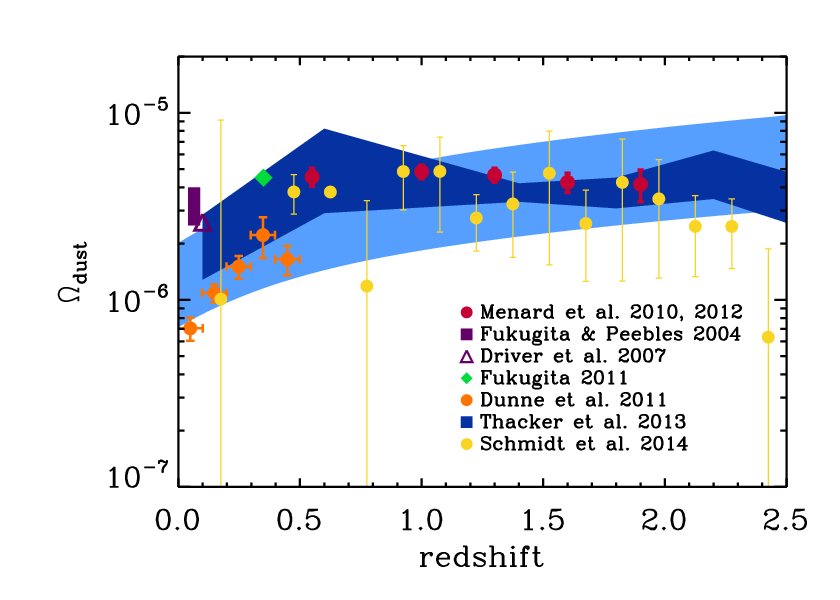
As an application of our models we also derive the fractional cosmic dust density $\Omega_{\rm dust}$ of galaxies from the fitting results. Following [48], the $\Omega_{\rm dust}$ for galaxies is given by

where $\rho_{0}$ is the current cosmic critical density, $\Phi(L,z)$ is the luminosity function, and $M_{\rm dust}$ is the dust mass with IR luminosity $L$ with temperature assumed to be 35$K$ that we fix in the power spectrum model. We make use of equation (4) of [19] to estimate $M_{\rm dust}$ from IR luminosity [48]. Also, we assume the dust opacity $\kappa_{d}$ takes the form as $\kappa_{d}=A_{\kappa}\nu^{\beta_{d}}$, where $\beta_{d}=2$ is the dust emissivity spectral index, and $A_{\kappa}$ is the normalization factor which is estimated by $\kappa_{d}=0.07\pm 0.02\ \rm m^{2}kg^{-1}$ at 850 $\mu$m [17, 28].

We show $\Omega_{\rm dust}$ as a function of redshift in Figure 11. The blue shaded region is the 1$\sigma$ range of the $\Omega_{\rm dust}$ from the FIR. We also show the other measurements for comparison. The orange squares are from the H-ATLAS dust mass function as measured in [18], and the other data are based on the extinction measurements of the SDSS and 2dF surveys [36, 37, 20, 21, 16]. We find our $\Omega_{\rm dust}$ result from galaxies is consistent with the other measurements, which has $\Omega_{\rm dust}$ increasing at higher redshift.

References

- [1] Amblard, A., Cooray, A., Serra, P., et al. 2010, A&A, 518, L9
- [2] Amblard, A., et al. 2011, Nature, 470, 510
- [3] Arendt, R. G., Fixsen, D. J., & Moseley, S. H. 2000, ApJ, 536, 500
- [4] Ashby, M. L. N., et al. 2009, ApJ, 701, 428
- [5] Bertin, E. & Arnouts, S. 1996, A&AS, 117, 393
- [6] Bethermin, M., Dole, H., Lagache, G., et al. 2011, A&A, 529, A4
- [7] Cantalupo, C. M., et al. 2010, ApJS, 187, 212
- [8] Cappelluti, N., Kashlinsky, A., and Arendt, R. G., et al. 2012, ApJ, 769, 68
- [9] Chapman, J. F. & Wardle, M. 2006 MNRAS, 371, 513
- [10] Carollo, D., et al. 2010, ApJ, 712, 692–727
- [11] Cooray, A., Sheth, R.K. 2002, PR, 372, 1
- [12] Cooray, A., et al. 2012, Nature, 490, 514
- [13] Courteau, S., et al. 2011, ApJ, 739, 20
- [14] De Bernardis, F., & Cooray, A. 2012, ApJ, 760, 14
- [15] Dole, H., Lagache, G., Puget, J.-L., et al. 2006, A&A, 451, 417
- [16] Driver, S. P., et al. 2007, MNRAS, 379, 1022
- [17] Dunne, L. , Eales, S. A. , Edmunds, M. G. , et al. 2000, MNRAS, 315, 115
- [18] Dunne, L. , Gomez, H. , da Cunha, E. S., et al. 2010, MNRAS, 417, 1510
- [19] Fu, H., Jullo, E., Cooray, A., et al. 2012, ApJ, 753, 12
- [20] Fukugita, M., Peebles P. J. E., 2004, ApJ, 616, 643
- [21] Fukugita, M., 2011, arXiv, arXiv:1103.4191
- [22] Gonzalez, A. H., Zabludoff, A. I. & Zaritsky, D. 2005, ApJ, 618, 195-213
- [23] Gong, Y., & Chen, X. 2007, PRD, 76, 123007
- [24] Griffin, M. J. , Abergel, M. J. , Abreu, A. , et al. 2010, A&A, 518, L3
- [25] Helgason, K., Ricotti, M., & Kashlinsky, A. 2012, ApJ, 752, 113
- [26] Hivon, E., et al. 2002, ApJ, 567, 2
- [27] Hwang, H.S., Elbaz, D. , Magdis, G. , et al., 2010, MNRAS, 409, 75
- [28] James, A. , Dunne, L. et al., 2002 MNRAS, 335, 753
- [29] Kashlinsky, A., Arendt, R. G., Mather, J., & Moseley, S. H. 2005, Nature, 438, 45
- [30] Kashlinsky, A., Arendt, R. G., Mather, J., & Moseley, S. H. 2007, ApJL, 654, L5
- [31] Kashlinsky, A., Arendt, R. G., Ashby, M. L. N., Fazio, G. G., Mather, J., & Moseley S. H. 2012, ApJ, 753, 63
- [32] Krick, J. E., & Bernstein, R. A. 2007, ApJ, 134, 466-493
- [33] Lee et al., ApJ 695, 368 (2009)
- [34] Lin, Y. T., Mohr, J. J., & Stanford, S. A. 2004, ApJ, 610, 745-761
- [35] Matsumoto, T., Seo, H. J., Jeong, W.-S., Lee, H. M., Matsuura, S., Matsuhara, H., Oyabu, S., Pyo, J., et al. 2011, ApJ, 742, 124
- [36] Menard B., Scranton R., Fukugita M., Richards G., 2010, MNRAS, 405, 1025
- [37] Menard, B., & Fukugita, M. 2012, ApJ, 754, 116
- [38] Metropolis, N., Rosenbluth, A. W., Rosenbluth, M. N., Teller, A. H., & Teller, E. 1953, JCP, 21, 1087
- [39] Navarro, J. F., Frenk, C. S., White, S. D. M. 1997, ApJ, 490, 493
- [40] Oliver, S. J., Wang, L., Smith, A. J., Altieri, B., Amblard, A., et al. 2010, A&A, 518, L21
- [41] Ott, S. 2010, in Astronomical Society of the Pacific Conference Series, Vol. 434, Astronomical Data Analysis Software and Systems XIX, ed. Y. Mizumoto, K.-I. Morita, & M. Ohishi, 139
- [42] Pillbratt, G. L., et al. 2010, A&A, 518, L1
- [43] Planck Collaboration and Ade, P. A. R., Aghanim, N., Armitage-Caplan, C., Arnaud, M., Ashdown, M., Atrio-Barandela, F., Aumont, J., Baccigalupi, C., Banday, A. J., et al. 2014,A&A,571, A16
- [44] Purcell, C. W., Bullock, J. S. & Zentner, A. R. 2008, MNRAS, 391, 550-558
- [45] Schmidt, S., Menard, B., et al., 2014, MNRAS 446, 2696
- [46] Shang, C., et al. 2011, arXiv:1109.1522
- [47] Sheth, R. K., Tormen, G. 1999, MNRAS, 308, 119
- [48] Thacker, C., Cooray, Smidt, et al. 2013, ApJ, 768, 58
- [49] Viero, M. P., Wang, L., Zemcov, M., et al. 2013, ApJ, 772, 77
- [50] Yue, B., Ferrara, A., Salvaterra, R., Xu, Y., & Chen, X. 2013, MNRAS, 433, 1556–1566
- [51] Yue, B., Ferrara, A., Salvaterra, R., Xu, Y., & Chen, X. 2014, MNRAS, 440, 1263-1273
- [52] Zemcov, M. and Smidt, J. and Arai, T. and Bock, J. and Cooray, A., et al. 2014, Science, 346, 732-735