Selection effects in Gamma Ray Bursts correlations: consequences on the ratio between GRB and star formation rates

GRBs are the farthest sources, seen up to redshift $z=9.46$ [13], and if emitting isotropically they are also the most powerful, (with $E_{iso}\leq 10^{54}erg\ s^{-1}$), objects in the Universe. Notwithstanding the variety of their peculiarities, some common features may be identified by looking at their light curves. A crucial breakthrough in this area has been the observation of GRBs by the Swift satellite, launched in 2004. With the instruments on board, the Burst Alert Telescope (BAT, 15-150 keV), the X-Ray Telescope (XRT, 0.3-10 keV), and the Ultra-Violet/Optical Telescope (UVOT, 170-650 nm), Swift provides a rapid follow-up of the afterglows in several wavelengths with better coverage than previous missions. Swift observations have revealed a more complex behavior of the light curves afterglow [46, 57] that can be divided into two, three and even more segments in the afterglows. The second segment, when it is flat, is called plateau emission. A significant step forward in determining common features in the afterglow light curves was made by fitting them with an analytical expression [66], called hereafter W07. This provides the opportunity to look for universal features that could provide a redshift independent measure of the distance from the GRB, as in studies of correlations between GRB isotropic energy and peak photon energy of the $\nu F_{\nu}$ spectrum, $E_{iso}-E_{peak}$, [40, 1], the beamed total energy $E_{\gamma}-E_{peak}$ [26, 27], the Luminosity-Variability, L-V [45, 24], L-$E_{peak}$ [68] and Luminosity- $\tau$ lag [58].
Dainotti et al. (2008, 2010), using the W07 phenomenological law for the light curves of long GRBs, discovered a formal anti-correlation between the X-ray luminosity at the end of the plateau $L_{X}$ and the rest frame plateau end-time, $T^{*}_{a}=T^{obs}_{a}/(1+z)$, where $T^{*}_{a}$ is in seconds and $L_{X}$ is in erg/s. The normalization and the slope parameters $a$ and $b$ are constants obtained by the D’Agostini fitting method [14]. Dainotti et al. (2011a) attempted to use the LT correlation as a possible redshift estimator, but the paucity of the data and the scatter prevents from a definite conclusion at least for a sample of 62 GRBs. In addition, a further step to better understand the role of the plateau emission has been made with the discovery of new significant correlations between $L_{X}$, and the mean luminosities of the prompt emission, $<L_{\gamma,prompt}>$ [19]. The LT anticorrelation is also a useful test for theoretical models such as the accretion models, [8, 9], the magnetar models [22, 3, 4, 54, 55, 56], the prior emission model [67], the unified GRB and AGN model [44] and the fireshell model [32]. Moreover, [30] and [64] consider both the LT and the $L_{X}$-$<L_{\gamma,prompt}>$ correlation to discriminate among several models proposed for the origin of plateau. In [38] and in [63] a smooth energy injection through the reverse shock has been presented as a plausible explanation for the origin of the LT correlation. Furthermore, also other authors were able to reproduce and use the LT correlation to extend it in the optical band [28], to extrapolated it into correlations of the prompt emission [61] and to use the same methodology to build an analogous correlation in the prompt [52]. Finally, it has been applied as a cosmological tool [10, 11, 20, 51]. Impacts of detector thresholds on cosmological standard candles have also been considered [59, 48, 49, 47, 7]. However, because of large dispersion [6, 69] and absence of good calibration none of these correlations allow the use of GRBs as good standard candles as it has been done e.g. with type Ia Supernovae. An important statistical technique to study selection effects for treating data truncation in GRB correlations is the [23] method. Another way to study the same problem in GRB correlations, derived modeling the high-energy properties of GRBs, have been reported in Butler et al. (2010). In the latter paper it has been shown that well-known examples of these correlations have common features indicative of strong contamination by selection effects. We compare this procedure with the method introduced by Efron & Petrosian (1992) and applied to the LT correlation [21]. The paper is organized as follows: section II introduces the relation between GRB and SFR, section II.1 is dedicated to the analysis of a GRB scaling relation, in particular we consider the LT correlation as an example, but the procedure described can be adopted for any other correlation. In section III we describe how to build the GRB samples, in section IV we analyze the redshift evolution of the slope and normalization of the LT correlation. In section V we study the selection effects related to simulated samples assuming different normalization and slope values. Then, in section VI we draw conclusions on the intrinsic slope of the LT correlation and on the evaluation of the redshift-dependent ratio between GRB and star formation rates.

In order to understand the relation between GRBs and the star formation, it is often assumed that the GRB rate (RGRB) is proportional to the SFR then the predicted distribution of the GRB redshift is compared to the observed distribution [62, 42, 65, 50, 43, 33, 15, 37, 12, 41]. However, this relationship is not an easy task to handle, because some studies show that GRBs do not seem to trace the star formation unbiasedly [40]. Namely, the ratio between the RGRB and SFR, RGRB/SFR, increases with redshift [34, 70] significantly. This means that GRBs are more frequent for a given star formation rate density at earlier times. In fact, while observations consistently show that the comoving rate density of star formation is nearly constant in the interval $1\leq z\leq 4$ [31], the comoving rate density of GRBs appears evolving distinctly. In our approach we explicitly take into consideration this issue when we fit the observed GRB rate with the model. Selection effects involved in a GRB sample are of two kinds : the GRB detection and localization; and the redshift determination through spectroscopy and photometry of the GRB afterglow or the host galaxy. These problems have been object of extensive study in literature [5, 25, 29]. Moreover, the Swift trigger, is very complex and the sensitivity of the detector is very difficult to parameterize exactly [2], but in this case not dealing with prompt peak energy we do not have to take into consideration the double truncation present in data [40]. In the case of plateau it is easier, since an effective luminosity threshold appears to be present in the data which can be approximated by a $0.3-10$ keV energy flux limit $F_{lim}\equiv 2\times 10^{−12}$ erg $cm^{−2}$ $s^{−1}$ [21]. The luminosity threshold is then $L_{lim}=4\pi D_{L}^{2}(z,\Omega_{M},H_{0})F_{lim}$, where $D_{L}$ is the luminosity distance to the burst. Throughout the paper, we assume a flat universe with $\Omega_{M}=0.28$, $\Omega_{\lambda}=0.72$ and $H_{0}$=70 km $s^{−1}$ $Mpc^{−1}$. In our approach below several models are considered and then the one that best matches the GRB rate with star formation rate has been chosen.

The GRBs rate given by Equation 8 has been derived by implicitly assuming that all the GRBs can be detected notwithstanding their observable properties. This is actually not the case. As an example, we will consider hereafter the LT correlation although the formalism and the method we will develop can be easily extended to whatever scaling law. For the LT case, there are two possible selection effects. First, each detector has an efficiency which is not the same for all the luminosities. Only GRBs with $\lambda>\lambda_{L}$, where $\lambda_{L}$ is the lowest detectable luminosity for a given instrument, can be detected while all the GRBs with $\lambda$ larger than a threshold luminosity $\lambda_{U}$ will be found.

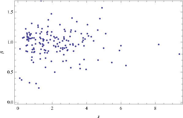
Moreover, it is likely that the efficiency of the detector is not constant, but is rather a function of the luminosity. We will therefore introduce an efficiency function $\mathcal{E}_{\lambda}(\lambda)$ whose functional expression is not known in advance, but can only take values in the range (0,1). A second selection effect is related to the time duration of the GRB. Indeed, in order to be included in the sample used to calibrate the LT correlation, the GRB afterglow has to be measured over a sufficiently long time scale to make possible to fit the data and extract the relevant quantities. If $\tau$ is too small, as it has been shown in Dainotti et al. (2013a) the minimum rest frame time is 14 s, few points will be available for the fit, while, on the contrary, large $\tau$ values will give rise to afterglow light curves which could be well sampled by the data. Again, we can parametrize these effects introducing a second efficiency function $\mathcal{E}_{\tau}(\tau)$ so that the final observable rate is the following:

We point out that our formulation, which takes into account of the efficiency functions $\mathcal{E}_{\lambda}(\lambda)$ and $\mathcal{E}_{\lambda}(\tau)$ in the final observed GRB rate is similar to the approach by Robertson & Ellis (2012) in Equation 1, in which the additional factor K is presented. K is equivalent to our $\mathcal{E}_{\lambda}(\lambda)$ and $\mathcal{E}_{\lambda}(\tau)$.

It is worth noting that Equation 10 is actually still a simplified description. Indeed, it is in principle possible that other selection effects take place involving observable quantities not considered here, as for example $\beta$ and the redshift. However, these parameters enter in the determination of $\lambda$ so that one can (at least in a first order approximation) convert selection cuts on them in a single efficiency function depending only on $\lambda$ (for the dependence of the flux on the redshift see left panel of Fig. 3). However, as we can see from Fig. 3 $\beta$ is constant with redshift, and there is no correlation between those two quantities, in fact the Spearman correlation coefficient is $\rho=-0.062$. Nevertheless, Equation 10 provides a reasonably accurate description of the observable GRB rate.

In order to evaluate Equation 10 there are different quantities to determine. First, we need to set the scaling coefficients ($\alpha_{0}$, $\alpha_{\tau}$, $\alpha_{\zeta}$) and the intrinsic scatter $\sigma_{int}$. Second, the mean and variance of the $\tau$ distribution ($\tau_{0}$,$\sigma_{\tau}$) has to be given. Finally, an expression for the cosmic SFR $\dot{\rho}_{*}(z)$ has to be assigned. None of these quantities is actually available. In principle, one could assume a SFR law and fit for the model parameters to a large enough GRBs sample with measured ($\lambda$, $\tau$, $\zeta$) values. To this end, one should know the selection function $\mathcal{E}_{\lambda}(\lambda)\mathcal{E}_{\tau}(\tau)$ which is not the case. Studies of how light curves would appear to a gamma-ray detector here on Earth have been performed [36]. In this paper the prompt emission pulses are investigated and the conclusion is that even a perfect detector that observes over a limited energy range would not faithfully measure the expected time dilation effects on a GRB pulse as a function of redshift.

Nevertheless, here we study detector threshold effects on afterglow properties. Our aim is to investigate how the ignorance of the efficiency function bias the estimate of the correlation coefficients. We can therefore rely on simulated samples based on a realistic intrinsic rate. We proceed as schematically outlined below.

• (i)

  We assume that the available data represent reasonably well the intrinsic $\tau$ distribution so that we can infer ($\tau_{0}$, $\sigma_{\tau}$) from the data themselves. We set $\tau_{L,U}=\tau_{0}\pm 5\sigma_{\tau}$ thus symmetrically cutting the Gaussian distribution at its extreme ends.

• (ii)

  Based on the shape of the cosmic SFR [31], we assume a broken power law for the comoving GRB rate density:

  $$\dot{\rho}_{*}(z)\propto\begin{cases}(1+z)^{g_{0}}&z\leq z_{0}\\ (1+z)^{g_{1}}&z_{0}\leq z\leq z_{1}\\ (1+z)^{g_{2}}&z\geq z_{1}\end{cases}$$

  (11)

  where the relative normalizations are set so that $\dot{\rho}_{*}(z)$ is continuous at $z_{0}=0.97$ and $z_{1}$ and $(z_{0},z_{1})=(0.97,4.50)$, $(g_{0},g_{1},g_{2})=(3.4,-0.3,-8.0)$. Moreover, besides the equation 11, we employed other shapes of the SFR [39, 53, 35] to obtain the observed GRBs rate density. The one used by [39] is:

  $$\dot{\rho}(z)=a+b\times Log(1+z).$$

  (12)

  The a and b parameters are :

  $$(a,b)=\begin{cases}(-1.70,3.30)&z\leq 0.993\\ (-0.727,0.0549)&0.993\leq z\leq 3.80\\ (2.35,-4.46)&z\geq 3.80\\ \end{cases}$$

  (13)

  Robertson & Ellis (2012) defined the SFR as:

  $$\dot{\rho}(z)=\frac{a+b(z/c)^{f}}{1+(z/c)^{d}}+g,$$

  (14)

  where they have $a=0.009M_{\odot}yr^{-1}Mpc^{-3}$, $b=0.27M_{\odot}yr^{-1}Mpc^{-3}$, $c=3.7$, $d=7.4$, and $g=10^{-3}M_{\odot}yr^{-1}Mpc^{-3}$.

  Instead, Kistler et al. (2013) defined the SFR as :

  $$\dot{\rho}(z)=\dot{\rho}_{0}\times[(1+z)^{a\psi}+(\frac{1+z}{B})^{b\psi}+(\frac{1+z}{C})^{c\psi}]^{\frac{1}{\psi}},$$

  (15)

  with slopes $a=3.4$, $b=-0.3$, and $c=-2.5$, breaks at $z_{1}=1$ and $z_{2}=4$ corresponding to $B=(1+z_{1})^{1-\frac{a}{b}}\sim 5160$ and $C=(1+z_{1})^{\frac{(b-a)}{c}}\times(1+z_{2})^{\frac{(1-b)}{c}}\sim 11.5$, and $\psi=-10$.

  Finally, we compare the fitted functions obtained with these four methods with our data distribution. The most realible fits for our parameters is the SFR used by Li (2008), see Fig. 4 where the best fit among linear (upper panel) and polynomial (lower panel) $\epsilon(\lambda)$ functions are considered. Moreover, we adopted the constraints for the redshift dependent ratio between SFR and GRB rate adopted by Robertson & Ellis (2012). In this paper a modest evolution (e.g.,$\Psi(z)\approx(1+z)^{\alpha}$) with $-0.2\leq\alpha\leq 1.5$, where the peak probability occurs for $\alpha\approx 0.5$ is consistent with the long GRB prompt data ($P\approx 0.9$). These values can be explained if GRBs occur primarily in low-metallicity galaxies which are proportionally more numerous at earlier times. We note that in our approach we assumed no evolution at low redshift for $z\leq 0.99$ consistently with the posterior probability in Robertson & Ellis (2012) in which no evolution is possible at the 2-$\sigma$ level. However, because a constant $\Psi(z)$ is also ruled out [53], then we fit the normalization parameters and the evolution factors obtaining $\Psi(z)\approx(1+z)^{-0.2}$ for $0.993\leq z\leq 3.8$ and $\Psi(z)\approx(1+z)^{0.5}$ for $z\geq 3.8$. These values of the evolution are compatible with Robertson et al. (2012). Regarding the observed GRB rate we obtained that the best efficiency functions are possible both for two polynomial and two linear as we show in Fig. 4. Table 1 and 2 show the probability that the density rate match the afterglow plateau GRB rate assuming those efficiency functions

• (iii)

  For given ($\alpha_{0}$, $\alpha_{\tau}$, $\alpha_{\zeta}$, $\sigma_{int}$) values, we divide the 2D space ($\lambda$, $z$) in $\mathcal{M}$ cells and, for each cell, compute the fraction of GRBs in it as:

  $$f_{sim}(\lambda_{i},z_{i})=\frac{\int_{\lambda_{i}-\Delta\lambda}^{\lambda_{i}+\Delta\lambda}d\lambda\int_{z_{i}-\Delta z}^{z_{i}+\Delta z}dz\frac{d\mathcal{N}}{d\lambda dz}}{\int_{\lambda_{min}}^{\lambda_{max}}d\lambda\int_{z_{min}}^{z_{max}}dz\frac{d\mathcal{N}}{d\lambda dz}}$$

  (16)

  where we set

  $$(\lambda_{min},\lambda_{max})=(42.0,52.0),(z_{min},z_{max})=(0,10).$$

  (17)

  We find more efficient to change variable from $z$ to $\zeta$ when dividing the 2D space in $10\times 10$ square cells.

• (iv)

  For each given cell, we generate $\mathcal{N}_{ij}=f_{sim}(\lambda_{i},\zeta_{j})\times\mathcal{N}_{sim}$ GRBs (with $\mathcal{N}_{sim}$ the total number of objects to simulate) by randomly sampling ($\lambda$, $\zeta$) within the cell boundaries and computing $\tau$ by solving Eq. 1.

• (v)

  To take into account of the selection effects, for each GRB, we generate two random numbers ($u_{\tau}$,$u_{\lambda}$) uniformly sampling the range (0, 1) and only retain the GRB if $u_{\tau}\leq\mathcal{E}_{\tau}(\tau)$ and $u_{\lambda}\leq\mathcal{E}_{\lambda}(\lambda)$. Note that, as a consequence of this cut, the final number $\mathcal{N}_{obs}$ of observed GRBs is smaller than the input one $\mathcal{N}_{sim}$.

• (vi)

  Finally, for each one of the $\mathcal{N}_{obs}$ selected GRBs, we generate new ($\tau_{obs}$, $\lambda_{obs}$) values extracting from Gaussian distributions centered on the simulated ($\tau$, $\lambda$) values and with a 1% variance. We also associate to each GRB an error set in such a way to be similar to what is actually obtained for GRBs having comparable ($\tau$, $\lambda$) values.

The above procedure allows us to build simulated GRBs sample taking into account both the intrinsic properties of any scaling relation and the selection effects induced by the instrumental setup. Moreover, we have referred to an actual GRBs sample in order to set both the limits on ($\tau$, $\zeta$, $\lambda$) and the typical measurement errors. Therefore, we can rely on these simulated samples to investigate the impact of selection effects on the recovered slope and intrinsic scatter of the given correlation. To this end, the last ingredient we need is a functional expression for the efficiency functions. Since these are largely unknown, we are forced to make some arbitrary guess. Therefore, we consider two different cases. First, we assume that there is no selection on $\tau$ , i.e. we set $\mathcal{E}_{\tau}=1$. Two functional expressions are then used for $\mathcal{E}_{\lambda}$, namely a power law:

and a fourth order polynomial, i.e. :

with $\tilde{\lambda}=(\lambda-\lambda_{L})/(\lambda_{U}-\lambda_{L})$. We try different arbitrary choices for the parameters entering both expressions of $\mathcal{E}_{\lambda}$ in order to investigate to which extent the results depend on the exact choice of the efficiency function, see Fig. 5. In a second step, we abandon the assumption $\mathcal{E}_{\tau}=1$, to assume for it the same functional expression used for $\mathcal{E}_{\lambda}$, with the same choices for the parameters, but different upper and lower limits depending on $\tau_{U}$ and $\tau_{L}$, see Fig. 6.

As we have already mentioned in the previous paragraph the polynomial and the linear model for the $\epsilon(\lambda)$ are unknown, then assumptions need to be made. We chose these forms, because both normalization and slope of the LT correlation depend on the redshift either with a polynomial or with a simple power law. Therefore, these choices for the selection functions take into account of this redshift dependence. Namely, we consider a model redshift dependence because of the corresponding dependence of both luminosity and time. This has been already shown in Dainotti et al. (2013a) and currently inthe middle panel of Fig. 3 for the updated data sample. To study the behavior of the redshift evolution we plot the slope and the normalization values versus the redshift. These are obtained from the average values for the data set divided into 5 bins, see figure 7 and into 12 bins, see figure 8. As we can see from both figures 7 and 8 the normalization parameter $\alpha_{0}$ decreases as the redshift increases, while the slope parameter $\alpha_{\tau}$ shows the opposite trend. Goodness of the fits is given by the probability $P=0.79$ for the data set divided in 5 bins and $P=0.87$ for the one divided into 12 bins for the linear case, while for the polynomial model $P=0.99$ and $P=0.94$ for the data set divided in 5 and 12 bins respectively. These results show that both polynomial and linear fit are possible.

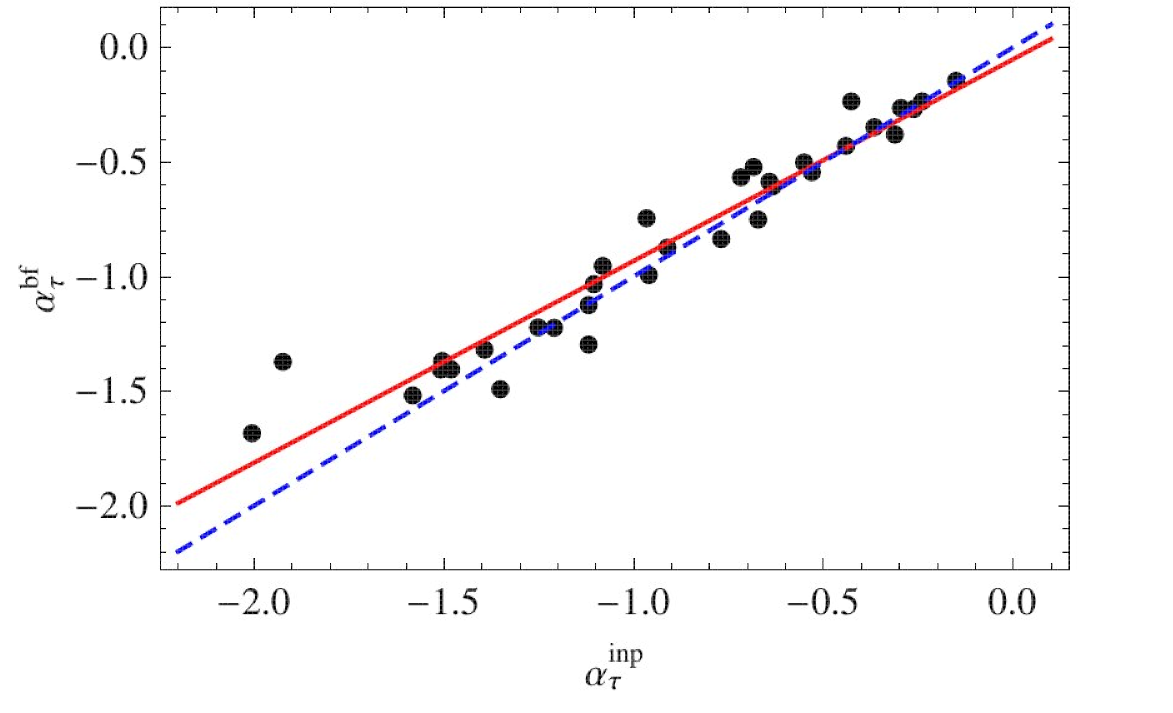
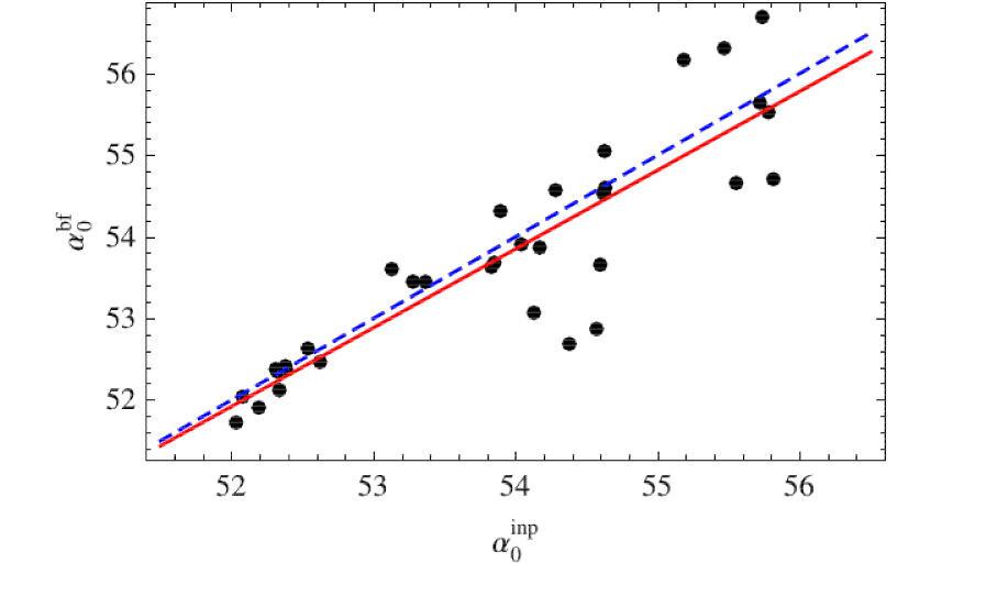
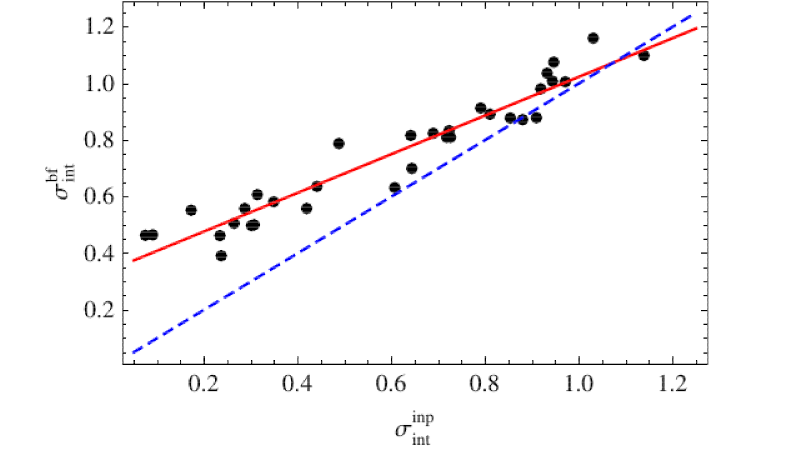
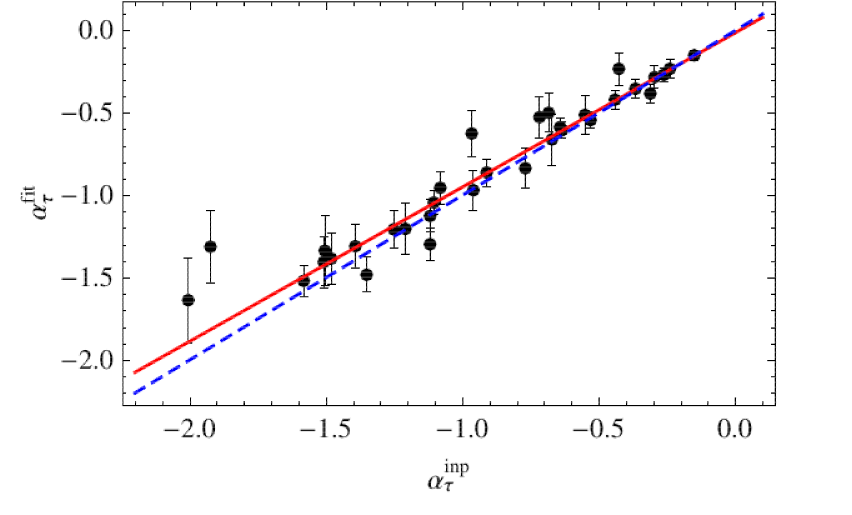
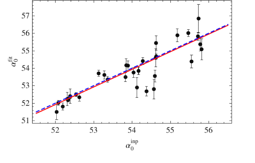
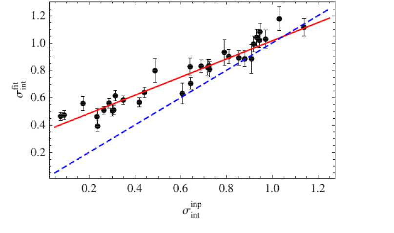
The simulated samples generated as described above are input to the same Bayesian fitting procedure we use with real data. For each input ($\alpha_{\tau}$, $\alpha_{\zeta}$, $\alpha_{0}$, $\sigma_{int}$) parameters, we simulate $\sim 50$ GRBs sample setting $\mathcal{N}_{sim}=200$, while the number of observed GRBs depend on the efficiency function used. We fit these samples assuming no redshift evolution in Eq. 1, i.e. forcing $\alpha_{\zeta}=0$ in the fit so that, for each simulated sample, the fitting procedure returns both the best fit and the median and 68% confidence range of the parameters ($\alpha_{\tau}$, $\alpha_{0}$, $\sigma_{int}$). In order to investigate whether the selection effects impact the recovery of the input scaling laws, we fit linear relations of the form:

where $x_{inp}$ is the input value and $x_{f}$ can be either the best fit (denoted as $x_{bf}$) or the median $x_{fit}$ value. When fitting the above linear relation, we use the $\chi^{2}$ minimization for $x_{bf}$, while a weighted fit is performed for $x_{fit}$ with weights $\omega_{i}=1/\sigma_{i}^{2}$ where $\sigma_{i}$ is the symmetrized $1\sigma$ error. Note that the label $i$ here runs over the simulations performed for each given efficiency function.

Here we built a general method to evaluate selection effects for GRB correlations not knowing a priori the efficiency function of the detector used. We have tested this method on the LT correlation. We chose a set of GRBs and assuming Gaussian distributions for the variables involved, for luminosity and time, and also a particular shape for the GRBs rate density. We simulated a mock sample of data in order to consider the selection effects of the detectors. As we can see in paragraph III assuming the correct observed GRBs rate density shape was not an easy task. In fact, we explored different methods [39, 53, 35, 31] that use several SFR shapes to understand which one best matches the afterglow plateau data distribution including the selection functions, see Fig. 4. The most reliable fits for the GRB plateau data is the SFR used by Li (2008), while the best efficiency functions for $\epsilon(\lambda)$ that match the GRB density rate can be both two polynomial and two linear, see Fig. 4. Table 1 and 2 show the probability that the density rate fits the afterglow plateau GRB rate assuming those efficiency functions. However, we assumed there could be selection effects both for luminosity and time. In particular, the bias is roughly the same whichever monotonic efficiency function for the luminosity detection $\mathcal{E}_{\lambda}$ is taken. From Table 3 and 4 we show that the relative biases, $\frac{\Delta_{x}}{x}$, both in the linear and the polynomial case, give very small values from $0.2\%$ to $0.9\%$, with the only exception of $1$ polynomial function, in which the bias is $18\%$, thus giving $P=10\%$ of having larger bias than $5\%$. If we consider selection cuts on both $\tau$ and $\lambda$ we notice in Table 5 that number of bias whose value is greater than $5\%$ are 4, thus increasing the probability of having such biases ($P\sim 40$%). In addition, we studied selection effects in the LT correlation assuming also a combination of the luminosity and time detection efficiency functions. Different values for the parameters of the efficiency functions in the detectors are taken into account as described in the paragraph V. This gives distinct fit values that inserted in Equation 20 allow to study the scattering of the correlation and its selection effects. We have quantitatively confirmed the existence of the $L_{X}-T^{*}_{a}$ correlation with the same intrinsic slope as in Dainotti et al. (2013a) if appropriate selection functions are chosen. In particular, when $\frac{\Delta_{x}}{x}$ are larger than $6\%$, than the slope of the correlation is farther from $-1.0$ compared to cases in which $\frac{\Delta_{x}}{x}\leq 0.06$. The lowest $\frac{\Delta_{x}}{x}$ leads to ranges of $a=(0.94,0.99)$ thus showing full compatibility in 1 $\sigma$ with the intrinsic slope. Finally, the fact that the correlation is not generated by the biases themselves is a significant and further step towards considering a set of GRBs as standard candles and their possible and useful application as a cosmological tool.

This work made use of data supplied by the UK Swift Science Data Centre at the University of Leicester. We are particularly grateful to Cardone, V.F. for the initial contribution to this work. M.G.D. and S.N. are grateful to the iTHES Group discussions at Riken. M.D is grateful to the support from the JSPS Foundation, (No. 25.03786). N. S. is grateful to JSPS (No.24.02022, No.25.03018, No.25610056, No.26287056) $\&$ MEXT(No.26105521), R. D.V. is grateful to 2012/04/A/ST9/00083.

References

- [1] L. Amati, F. Frontera, and C. Guidorzi. Extremely energetic Fermi gamma-ray bursts obey spectral energy correlations. A&A, 508:173–180, December 2009. 10.1051/0004-6361/200912788.
- [2] D. L. Band. Postlaunch Analysis of Swift’s Gamma-Ray Burst Detection Sensitivity. ApJ, 644:378–384, June 2006. 10.1086/503326.
- [3] M. G. Bernardini, R. Margutti, J. Mao, E. Zaninoni, and G. Chincarini. The X-ray light curve of gamma-ray bursts: clues to the central engine. A&A, 539:A3, March 2012a. 10.1051/0004-6361/201117895.
- [4] M. G. Bernardini, R. Margutti, E. Zaninoni, and G. Chincarini. A universal scaling for short and long gamma-ray bursts: EX,iso - Eγ,iso - Epk. MNRAS, 425:1199–1204, September 2012b. 10.1111/j.1365-2966.2012.21487.x.
- [5] J. S. Bloom. Is the Redshift Clustering of Long-Duration Gamma-Ray Bursts Significant? AJ, 125:2865–2875, June 2003. 10.1086/374945.
- [6] N. R. Butler, J. S. Bloom, and D. Poznanski. The Cosmic Rate, Luminosity Function, and Intrinsic Correlations of Long Gamma-Ray Bursts. ApJ, 711:495–516, March 2010. 10.1088/0004-637X/711/1/495.
- [7] J. I. Cabrera, C. Firmani, V. Avila-Reese, G. Ghirlanda, G. Ghisellini, and L. Nava. Spectral analysis of Swift long gamma-ray bursts with known redshift. MNRAS, 382:342–355, November 2007. 10.1111/j.1365-2966.2007.12374.x.
- [8] J. K. Cannizzo and N. Gehrels. A New Paradigm for Gamma-ray Bursts: Long-term Accretion Rate Modulation by an External Accretion Disk. ApJ, 700:1047–1058, August 2009. 10.1088/0004-637X/700/2/1047.
- [9] J. K. Cannizzo, E. Troja, and N. Gehrels. Fall-back Disks in Long and Short Gamma-Ray Bursts. ApJ, 734:35, June 2011. 10.1088/0004-637X/734/1/35.
- [10] V. F. Cardone, S. Capozziello, and M. G. Dainotti. An updated gamma-ray bursts Hubble diagram. MNRAS, 400:775–790, December 2009. 10.1111/j.1365-2966.2009.15456.x.
- [11] V. F. Cardone, M. G. Dainotti, S. Capozziello, and R. Willingale. Constraining cosmological parameters by gamma-ray burst X-ray afterglow light curves. MNRAS, 408:1181–1186, October 2010. 10.1111/j.1365-2966.2010.17197.x.
- [12] D. Coward. Open issues with the gamma-ray burst redshift distribution. New A Rev., 51:539–546, September 2007. 10.1016/j.newar.2007.03.003.
- [13] A. Cucchiara, A. J. Levan, D. B. Fox, N. R. Tanvir, T. N. Ukwatta, E. Berger, T. Krühler, A. Küpcü Yoldaş, X. F. Wu, K. Toma, J. Greiner, F. E. Olivares, A. Rowlinson, L. Amati, T. Sakamoto, K. Roth, A. Stephens, A. Fritz, J. P. U. Fynbo, J. Hjorth, D. Malesani, P. Jakobsson, K. Wiersema, P. T. O’Brien, A. M. Soderberg, R. J. Foley, A. S. Fruchter, J. Rhoads, R. E. Rutledge, B. P. Schmidt, M. A. Dopita, P. Podsiadlowski, R. Willingale, C. Wolf, S. R. Kulkarni, and P. D’Avanzo. A Photometric Redshift of z ˜ 9.4 for GRB 090429B. ApJ, 736:7, July 2011. 10.1088/0004-637X/736/1/7.
- [14] G. D’Agostini. Fits, and especially linear fits, with errors on both axes, extra variance of the data points and other complications. ArXiv Physics e-prints, November 2005.
- [15] F. Daigne and R. Mochkovitch. The low-luminosity tail of the GRB distribution: the case of GRB 980425. A&A, 465:1–8, April 2007. 10.1051/0004-6361:20066080.
- [16] M. G. Dainotti, V. F. Cardone, and S. Capozziello. A time-luminosity correlation for -ray bursts in the X-rays. MNRAS, 391:L79–L83, November 2008. 10.1111/j.1745-3933.2008.00560.x.
- [17] M. G. Dainotti, R. Willingale, S. Capozziello, V. Fabrizio Cardone, and M. Ostrowski. Discovery of a Tight Correlation for Gamma-ray Burst Afterglows with ”Canonical” Light Curves. ApJ, 722:L215–L219, October 2010. 10.1088/2041-8205/722/2/L215.
- [18] M. G. Dainotti, V. Fabrizio Cardone, S. Capozziello, M. Ostrowski, and R. Willingale. Study of Possible Systematics in the L*X-T*a Correlation of Gamma-ray Bursts. ApJ, 730:135, April 2011a. 10.1088/0004-637X/730/2/135.
- [19] M. G. Dainotti, M. Ostrowski, and R. Willingale. Towards a standard gamma-ray burst: tight correlations between the prompt and the afterglow plateau phase emission. MNRAS, 418:2202–2206, December 2011b. 10.1111/j.1365-2966.2011.19433.x.
- [20] M. G. Dainotti, V. F. Cardone, E. Piedipalumbo, and S. Capozziello. Slope evolution of GRB correlations and cosmology. MNRAS, 436:82–88, November 2013a. 10.1093/mnras/stt1516.
- [21] M. G. Dainotti, V. Petrosian, J. Singal, and M. Ostrowski. Determination of the Intrinsic Luminosity Time Correlation in the X-Ray Afterglows of Gamma-Ray Bursts. ApJ, 774:157, September 2013b. 10.1088/0004-637X/774/2/157.
- [22] S. Dall’Osso, G. Stratta, D. Guetta, S. Covino, G. De Cesare, and L. Stella. Gamma-ray bursts afterglows with energy injection from a spinning down neutron star. A&A, 526:A121, February 2011. 10.1051/0004-6361/201014168.
- [23] B. Efron and V. Petrosian. A simple test of independence for truncated data with applications to redshift surveys. ApJ, 399:345–352, November 1992. 10.1086/171931.
- [24] E. E. Fenimore and E. Ramirez-Ruiz. Redshifts For 220 BATSE Gamma-Ray Bursts Determined by Variability and the Cosmological Consequences. ArXiv Astrophysics e-prints, April 2000.
- [25] F. Fiore, D. Guetta, S. Piranomonte, V. D’Elia, and L. A. Antonelli. Selection effects shaping the gamma ray burst redshift distributions. A&A, 470:515–522, August 2007. 10.1051/0004-6361:20077157.
- [26] G. Ghirlanda, G. Ghisellini, and D. Lazzati. The Collimation-corrected Gamma-Ray Burst Energies Correlate with the Peak Energy of Their Fnu Spectrum. ApJ, 616:331–338, November 2004. 10.1086/424913.
- [27] G. Ghirlanda, G. Ghisellini, and C. Firmani. Gamma-ray bursts as standard candles to constrain the cosmological parameters. New Journal of Physics, 8:123, July 2006. 10.1088/1367-2630/8/7/123.
- [28] G. Ghisellini, M. Nardini, G. Ghirlanda, and A. Celotti. A unifying view of gamma-ray burst afterglows. MNRAS, 393:253–271, February 2009. 10.1111/j.1365-2966.2008.14214.x.
- [29] D. Guetta and M. Della Valle. On the Rates of Gamma-Ray Bursts and Type Ib/c Supernovae. ApJ, 657:L73–L76, March 2007. 10.1086/511417.
- [30] R. Hascoët, F. Daigne, and R. Mochkovitch. The prompt-early afterglow connection in gamma-ray bursts: implications for the early afterglow physics. MNRAS, 442:20–27, July 2014. 10.1093/mnras/stu750.
- [31] A. M. Hopkins and J. F. Beacom. On the Normalization of the Cosmic Star Formation History. ApJ, 651:142–154, November 2006. 10.1086/506610.
- [32] L. Izzo, G. B. Pisani, M. Muccino, J. A. Rueda, Y. Wang, C. L. Bianco, A. V. Penacchioni, and R. Ruffini. A common behavior in the late X-ray afterglow of energetic GRB-SN systems. In A. J. Castro-Tirado, J. Gorosabel, and I. H. Park, editors, EAS Publications Series, volume 61 of EAS Publications Series, pages 595–597, July 2013. 10.1051/eas/1361095.
- [33] P. Jakobsson, A. Levan, J. P. U. Fynbo, R. Priddey, J. Hjorth, N. Tanvir, D. Watson, B. L. Jensen, J. Sollerman, P. Natarajan, J. Gorosabel, J. M. Castro Cerón, K. Pedersen, T. Pursimo, A. S. Árnadóttir, A. J. Castro-Tirado, C. J. Davis, H. J. Deeg, D. A. Fiuza, S. Mikolaitis, and S. G. Sousa. A mean redshift of 2.8 for Swift gamma-ray bursts. A&A, 447:897–903, March 2006. 10.1051/0004-6361:20054287.
- [34] M. D. Kistler, H. Yüksel, J. F. Beacom, and K. Z. Stanek. An Unexpectedly Swift Rise in the Gamma-Ray Burst Rate. ApJ, 673:L119–L122, February 2008. 10.1086/527671.
- [35] M. D. Kistler, H. Yuksel, and A. M. Hopkins. The Cosmic Star Formation Rate from the Faintest Galaxies in the Unobservable Universe. ArXiv e-prints, May 2013.
- [36] D. Kocevski and V. Petrosian. On the Lack of Time Dilation Signatures in Gamma-Ray Burst Light Curves. ApJ, 765:116, March 2013. 10.1088/0004-637X/765/2/116.
- [37] T. Le and C. D. Dermer. On the Redshift Distribution of Gamma-Ray Bursts in the Swift Era. ApJ, 661:394–415, May 2007. 10.1086/513460.
- [38] K. Leventis, R. A. M. J. Wijers, and A. J. van der Horst. The plateau phase of gamma-ray burst afterglows in the thick-shell scenario. MNRAS, 437:2448–2460, January 2014. 10.1093/mnras/stt2055.
- [39] L.-X. Li. The X-ray transient 080109 in NGC 2770: an X-ray flash associated with a normal core-collapse supernova. MNRAS, 388:603–610, August 2008. 10.1111/j.1365-2966.2008.13461.x.
- [40] N. M. Lloyd and V. Petrosian. Distribution of Spectral Characteristics and the Cosmological Evolution of Gamma-Ray Bursts. ApJ, 511:550–561, February 1999. 10.1086/306719.
- [41] J. Mao. A Theoretical Investigation of Gamma-ray Burst Host Galaxies. ApJ, 717:140–146, July 2010. 10.1088/0004-637X/717/1/140.
- [42] S. Mao and H. J. Mo. The nature of the host galaxies for gamma-ray bursts. A&A, 339:L1–L4, November 1998.
- [43] P. Natarajan, B. Albanna, J. Hjorth, E. Ramirez-Ruiz, N. Tanvir, and R. Wijers. The redshift distribution of gamma-ray bursts revisited. MNRAS, 364:L8–L12, November 2005. 10.1111/j.1745-3933.2005.00094.x.
- [44] R. S. Nemmen, M. Georganopoulos, S. Guiriec, E. T. Meyer, N. Gehrels, and R. M. Sambruna. A Universal Scaling for the Energetics of Relativistic Jets from Black Hole Systems. Science, 338:1445–, December 2012. 10.1126/science.1227416.
- [45] J. P. Norris, G. F. Marani, and J. T. Bonnell. Connection between Energy-dependent Lags and Peak Luminosity in Gamma-Ray Bursts. ApJ, 534:248–257, May 2000. 10.1086/308725.
- [46] P. T. O’Brien, R. Willingale, J. Osborne, M. R. Goad, K. L. Page, S. Vaughan, E. Rol, A. Beardmore, O. Godet, C. P. Hurkett, A. Wells, B. Zhang, S. Kobayashi, D. N. Burrows, J. A. Nousek, J. A. Kennea, A. Falcone, D. Grupe, N. Gehrels, S. Barthelmy, J. Cannizzo, J. Cummings, J. E. Hill, H. Krimm, G. Chincarini, G. Tagliaferri, S. Campana, A. Moretti, P. Giommi, M. Perri, V. Mangano, and V. LaParola. The Early X-Ray Emission from GRBs. ApJ, 647:1213–1237, August 2006. 10.1086/505457.
- [47] V. Petrosian. New Statistical Methods for Analysis of Large Surveys: Distributions and Correlations. In R. F. Green, E. Y. Khachikian, and D. B. Sanders, editors, IAU Colloq. 184: AGN Surveys, volume 284 of Astronomical Society of the Pacific Conference Series, page 389, 2002.
- [48] V. Petrosian and N. M. Lloyd. The nu Fnu Peak Energy of Gamma Ray Bursts, and its Correlation with Fluence and Peak Flux. In American Astronomical Society Meeting Abstracts, volume 30 of Bulletin of the American Astronomical Society, page 1380, December 1998.
- [49] V. Petrosian, N. Lloyd, and A. Lee. Cosmological Signatures in Temporal and Spectral Characteristics of Gamma-Ray Bursts. In J. Poutanen and R. Svensson, editors, Gamma-Ray Bursts: The First Three Minutes, volume 190 of Astronomical Society of the Pacific Conference Series, page 235, 1999.
- [50] C. Porciani and P. Madau. On the Association of Gamma-Ray Bursts with Massive Stars: Implications for Number Counts and Lensing Statistics. ApJ, 548:522–531, February 2001. 10.1086/319027.
- [51] S. Postnikov, M. G. Dainotti, X. Hernandez, and S. Capozziello. Nonparametric Study of the Evolution of the Cosmological Equation of State with SNeIa, BAO, and High-redshift GRBs. ApJ, 783:126, March 2014. 10.1088/0004-637X/783/2/126.
- [52] S. Qi and T. Lu. Toward Tight Gamma-Ray Burst Luminosity Relations. ApJ, 749:99, April 2012. 10.1088/0004-637X/749/2/99.
- [53] B. E. Robertson and R. S. Ellis. Connecting the Gamma Ray Burst Rate and the Cosmic Star Formation History: Implications for Reionization and Galaxy Evolution. ApJ, 744:95, January 2012. 10.1088/0004-637X/744/2/95.
- [54] A. Rowlinson, P. T. O’Brien, N. R. Tanvir, B. Zhang, P. A. Evans, N. Lyons, A. J. Levan, R. Willingale, K. L. Page, O. Onal, D. N. Burrows, A. P. Beardmore, T. N. Ukwatta, E. Berger, J. Hjorth, A. S. Fruchter, R. L. Tunnicliffe, D. B. Fox, and A. Cucchiara. The unusual X-ray emission of the short Swift GRB 090515: evidence for the formation of a magnetar? MNRAS, 409:531–540, December 2010. 10.1111/j.1365-2966.2010.17354.x.
- [55] A. Rowlinson, P. T. O’Brien, B. D. Metzger, N. R. Tanvir, and A. J. Levan. Signatures of magnetar central engines in short GRB light curves. MNRAS, 430:1061–1087, April 2013. 10.1093/mnras/sts683.
- [56] A. Rowlinson, B. P. Gompertz, M. Dainotti, P. T. O’Brien, R. A. M. J. Wijers, and A. J. van der Horst. Constraining properties of GRB magnetar central engines using the observed plateau luminosity and duration correlation. MNRAS, 443:1779–1787, September 2014. 10.1093/mnras/stu1277.
- [57] T. Sakamoto, J. E. Hill, R. Yamazaki, L. Angelini, H. A. Krimm, G. Sato, S. Swindell, K. Takami, and J. P. Osborne. Evidence of Exponential Decay Emission in the Swift Gamma-Ray Bursts. ApJ, 669:1115–1129, November 2007. 10.1086/521640.
- [58] B. E. Schaefer. Explaining the Gamma-Ray Burst Epeak Distribution. ApJ, 583:L71–L74, February 2003. 10.1086/368106.
- [59] A. Shahmoradi and R. Nemiroff. How Real Detector Thresholds Create False Standard Candles. In C. Meegan, C. Kouveliotou, and N. Gehrels, editors, American Institute of Physics Conference Series, volume 1133 of American Institute of Physics Conference Series, pages 425–427, May 2009. 10.1063/1.3155940.
- [60] B. E. Stern, Y. Tikhomirova, D. Kompaneets, R. Svensson, and J. Poutanen. An Off-Line Scan of the BATSE Daily Records and a Large Uniform Sample of Gamma-Ray Bursts. ApJ, 563:80–94, December 2001. 10.1086/322295.
- [61] J. Sultana, D. Kazanas, and K. Fukumura. Luminosity Correlations for Gamma-Ray Bursts and Implications for Their Prompt and Afterglow Emission Mechanisms. ApJ, 758:32, October 2012. 10.1088/0004-637X/758/1/32.
- [62] T. Totani. Cosmological Gamma-Ray Bursts and Evolution of Galaxies. ApJ, 486:L71–L74, September 1997. 10.1086/310853.
- [63] H. van Eerten. Self-similar relativistic blast waves with energy injection. MNRAS, 442:3495–3510, August 2014a. 10.1093/mnras/stu1025.
- [64] H. J. van Eerten. Gamma-ray burst afterglow plateau break time-luminosity correlations favour thick shell models over thin shell models. MNRAS, 445:2414–2423, December 2014b. 10.1093/mnras/stu1921.
- [65] R. A. M. J. Wijers, J. S. Bloom, J. S. Bagla, and P. Natarajan. Gamma-ray bursts from stellar remnants - Probing the universe at high redshift. MNRAS, 294:L13–L17, February 1998. 10.1046/j.1365-8711.1998.01328.x.
- [66] R. Willingale, P. T. O’Brien, J. P. Osborne, O. Godet, K. L. Page, M. R. Goad, D. N. Burrows, B. Zhang, E. Rol, N. Gehrels, and G. Chincarini. Testing the Standard Fireball Model of Gamma-Ray Bursts Using Late X-Ray Afterglows Measured by Swift. ApJ, 662:1093–1110, June 2007. 10.1086/517989.
- [67] R. Yamazaki. Prior Emission Model for X-ray Plateau Phase of Gamma-Ray Burst Afterglows. ApJ, 690:L118–L121, January 2009. 10.1088/0004-637X/690/2/L118.
- [68] D. Yonetoku, T. Murakami, T. Nakamura, R. Yamazaki, A. K. Inoue, and K. Ioka. Gamma-Ray Burst Formation Rate Inferred from the Spectral Peak Energy-Peak Luminosity Relation. ApJ, 609:935–951, July 2004. 10.1086/421285.
- [69] B. Yu, S. Qi, and T. Lu. Gamma-ray Burst Luminosity Relations: Two-Dimensional Versus Three-Dimensional Correlations. ApJ, 705:L15–L19, November 2009. 10.1088/0004-637X/705/1/L15.
- [70] H. Yüksel and M. D. Kistler. Enhanced cosmological GRB rates and implications for cosmogenic neutrinos. Phys. Rev. D, 75(8):083004, April 2007. 10.1103/PhysRevD.75.083004.