Precisely resolve energy-time entanglement by dual channel Fabry-Pérot interferometry
Abstract
Precisely resolving the continuous variable energy-time entanglement of paired photons is an important issue in quantum optics. The Fabry-Pérot interferometer provides a distinguished opportunity for this purpose if the single photon pulse’s self-interference is carefully avoided. A dual channel Fabry-Pérot interferometer is proposed and studied with the focus put upon higher order quantum interference effects. When the two channels are properly set up, it is capable of resolving the energy-time entanglement in detail analogously to that a usual Fabry-Pérot interferometer can resolve classical light’s spectrum. Variation form of the dual channel Fabry-Pérot interferometry is also discussed.
Energy-time entanglement, being an outstanding example of the entanglement between continuous variables [1, 2], has aroused the enthusiasm of many researchers in recent years. It provides convincing evidence against the local hidden variable (LHV) theory [3], and has potential important applications, such as the quantum cryptography and the quantum key distribution [4, 5, 6]. Ever since the Franson interferometry [7], many interesting schemes [8, 9, 10] have been proposed to examine the energy-time entanglement experimentally. Researchers have been working hard to improve the fringe visibilities [11, 12, 13, 14] for better contrast in the violation of the Bell inequality. Also, the highly non-local properties of energy-time entanglement have been investigated by various interferometric methods [15, 16, 17].
Intuitively, if two photons are energy-time entangled, the collapse of one photon’s wave packet onto some eigenstate specified by the detection methods at some time will necessarily mandate the time at which the other photon’s wave packet collapses [1]. Very often the total energy of such a photon pair is conserved with an uncertainty much less than that of an individual party. Usually, the energy-time entangled biphoton posses an experimental signature of strong correlations in the time at which they are registered as “clicks” in the detectors and their frequencies [18]. However, this type of correlations alone is not enough to serve as the proof for energy-time entanglement, nor does it provide the full information of the entanglement. On the other hand, two-photon Fabry-Pérot interferometer for time-bin entanglement [19] has already been studied thoroughly and we wonder whether an analogous interferometry exists for the very different entanglement of energy and time.
In this letter, we propose a dual channel Fabry-Pérot interferometer that has the ability to precisely resolve the energy-time entanglement of photon pairs. The aim of the proposed interferometry is not only to determine the existence of energy-time entanglement, but also to allow the actual experimental measurement of the fine structure of the energy-time entanglement in an unambiguous way. Since many of the potential quantum optics applications of the energy-time entanglement rely upon its essentially unlimited Hilbert space volume pertinent to the continuous variable entanglement, a method to precisely map out the entanglement is certainly of help.
The setup of this interferometer is sketched in Fig. 1 . It is composed of two arms of equal length, where a Fabry-Pérot interferometer is inserted into each arm. The two Fabry-Pérot interferometers have similar cavity lengths and all their mirrors are the same: planar, with field transmission coefficient and field reflection coefficient satisfying . Each arm is equipped with two single photon counting modules (SPCM) with assumed 100% quantum efficiency. A single photon pulse is to be registered as a click at time satisfying if the SPCM is placed at position , where is the field operator generating the single photon pulse and is the vacuum state. A key requirement is that the individual single photon pulse’s coherence time is less than the round trip time in the cavities in order to avoid self-interferences. The biphoton source is postulated to emit energy-time entangled photon pairs: a subscript or is attached to distinguish the photons coming down the left or right arm.
The discussion is carried out under the Heisenberg picture, where the field operator evolves in time. Suppose that when a pair of energy-time entangled photons is generated in free space, the field operator is given as in Eq.(1). Eq.(1) describes a photon pair that is perfectly energy-time entangled while both photons have only a single frequency component. All the counts registered by the SPCM & are coincidence counts in this case. Eq.(1) is regarded as an idealization to make the derivations simpler [20].
| (1) |
When the two Fabry-Pérot interferometers are inserted into the two arms separately as in Fig. 1, higher order quantum interference occurs for the two-photon state . First we turn our attention to the transmission that will induce coincidence counts in SPCM and , which is essentially a form of post-selection. The field operator describing such a transmission state is given in Eq.(2).
 |
| (2) |
We make the following observation as in Eq.(3), which is the consequence of energy–time entanglement [20].
| (3) |
From Eq.(4) it is clear that the transmission coincidence rate is mediated by the factor , which is analogous to the usual Fabry-Pérot transmission and leads to sharp “resonances”. The transmission coincidence rate can be calculated as in Eq.(5), when normalized to the coincidence rate if the two Fabry-Pérot interferometers are removed:
| (5) |
The “on–resonance” condition that leads to the maximum transmission coincidence is given in the following Eq.(6).
| (6) |
where is some positive integer number. Fig. 2 (a) & (b) present numerical simulation results for the transmission coincidence rates for and .
Eq.(4) and Eq.(5) are highly non-local results coming from higher order quantum interference as a consequence of the energy-time entanglement. Suppose that no entanglement exists, even if the pair of photons is always generated at the same time, the transmission coincidence counting rate would not vary with respect to the tiny change in the cavity length (change at the scale ). Moreover when entanglement does exist, Eq.(5) serves as the fully quantum mechanical prediction which refutes the prediction of an usual LHV model [20, 21, 22].
In the above discussions the frequencies of the two photons are specified. However it is not necessary to demand the photons to have fixed frequencies in order to make this interferometer behave. An adequate condition is that under the already mentioned postulation that , and then our analysis from Eq.(2) to Eq.(6) is still valid. This observation implies that this type of interferometry has the ability to detect the energy conservation of the biphotons within the accuracy of the inserted Fabry-Pérot interferometer’s linewidth, provided the fine experimental control over .
The transmission coincidence makes up only a small part of all the transmissions and such a post–selection process would necessarily throw away a lot of SPCM’s counts. More often, the clicks in SPCM and for the transmission will be separated by some time interval. For simplicity we put for the moment. Then the possible separation time between a click in and a click in is where positive means a click at is ahead of a click at while negative means a click at is ahead of a click at . The biphoton field operator governing the transmission for a specific interval is therefore calculated in Eq.(7).
| (7) |
Eq.(7) covers all the possibilities of the post–selection process for the transmission counts’ correlations. In other words, the total transmission biphoton field operator can be understood as . Eq.(7) implies that the non–coincidence counts are not just wastes but also carry vital information about the quantum interference as a result of the entanglement.
We now extend our analysis to the reflections registered by SPCM and . First the field operator for reflection coincidence is computed in Eq.(8).
| (8) |
which has an interesting tiny difference compared to the usual form of Fabry-Pérot’s reflection. Namely, the minus sign from the half wave loss disappears because in the two photon case it is multiplied twice. Fig. 2 (c) & (d) present numerical simulation results for the reflection coincidence rates.
 |
Not all the reflection counts on SPCM and are coincidences either. Similarly, assume for the moment. If the separation time between a click in and a click in is , then the corresponding biphoton field operator is computed in the following Eq.(9).
| (9) |
The correlation between the counts of SPCM and is also subject to the same quantum interferences. Keeping the definition of and the assumption of as above, we construct the biphoton field operator for the post–selection that a click in occurs at ahead of . When , is as in Eq.(10), while when , is as in Eq.(11).
| (10) |
| (11) |
This type of dual channel interferometry has close ties with weak values [23], and its description can be switched to an equivalent weak value formulation. It also shares some basic ideas with the geometric phases [8, 24]. It has a variation form whose schematic is presented in Fig. 3. By manipulating polarizations, dual channel interferometry for the energy–time entanglement is realized with only one actual Fabry-Pérot interferometer.
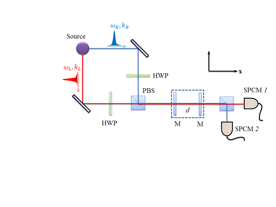 |
The design in Fig. 3 works on the same principle as that in Fig. 1 and yet has its distinct features. The artificial requirement of or is now automatically fulfilled. Eq. (7) applies here without modification. A numerical simulation for its performance in terms of coincidence rates is given in Fig. 4, where the signal strength drops significantly as the reflectivity of the cavity mirror increases. One way to gather more signal to counteract this drawback is through the utilization of all the ’s of Eq.7, and this method is similar to a recent method used to enhance the signal in the N00N state imaging experiment [25].
 |
For the sake of a succinct discussion, the assumed form of the entangled biphoton in Eq.(1) does not adequately address the intricate details of the energy–time entanglement. A simple but more realistic model is provided in Eq.(12), where contains the information about the energy–time entanglement.
| (12) |
An immediate observation is that Eq.(12) leads to energy uncertainties in the photons which Eq.(1) does not. The transmission coincidence of the biphoton in the form of Eq.(12) through the dual channel Fabry-Pérot interferometer is then computed in Eq.(13).
| (13) |
Provided the condition that and represent short single photon pulses, Eq.(13) means that the coincidence rate as a function of is essentially a windowed Fourier transform of . Therefore an experimental measurement similar to Fig. 2 or Fig. 4 will yield the spectral property of . Through this model analysis it is clear that the dual channel Fabry-Pérot interferometry has the ability to analyze the biphoton energy–time entanglement in a very analogous way that a usual Fabry-Pérot reveals the incident classical light’s frequency spectrum.
We discuss briefly three factors that will compromise the performance of this type of interferometry: phase noise, environmental noise and quantum detection efficiency. The phase noise of the optical field introduces unwanted stochasticity just like its role in the laser–atom interaction [26]. Environmental noise causes decoherence and may even lead to entanglement sudden death [27]. A low quantum detection efficiency will impede the data acquisition and smear the interference pattern’s visibility.
In conclusion, we have proposed a dual channel Fabry-Pérot interferometer and discussed in theory its properties. We have shown that it has the ability to precisely analyze the energy-time entanglement between a pair of photons and therefore it has the potential to become a standard tool for such tasks.
Acknowledgements.
The author acknowledges support from ONR and help from Dr. Harold Metcalf, which makes this work possible.References
- [1] L. K. Shalm, D. R. Hamel, Z. Yan, C. Simon, R. K. J., and T. Jennewein, Nature Physics 9, 19 (2013).
- [2] C. K. Law, I. A. Walmsley, and J. H. Eberly, Phys. Rev. Lett. 84, 5304 (2000).
- [3] J. Yin, Y. Cao, H.-L. Yong, J.-G. Ren, H. Liang, S.-K. Liao, F. Zhou, C. Liu, Y.-P. Wu, G.-S. Pan, L. Li, N.-L. Liu, Q. Zhang, C.-Z. Peng, and J.-W. Pan, Phys. Rev. Lett. 110, 260407 (2013).
- [4] W. Tittel, J. Brendel, H. Zbinden, and N. Gisin, Phys. Rev. Lett. 84, 4737 (2000).
- [5] I. Ali-Khan, C. J. Broadbent, and J. C. Howell, Phys. Rev. Lett. 98, 060503 (2007).
- [6] Z. Zhang, J. Mower, D. Englund, F. N. C. Wong, and J. H. Shapiro, Phys. Rev. Lett. 112, 120506 (2014).
- [7] J. D. Franson, Phys. Rev. Lett. 62, 2205 (1989).
- [8] A. K. Jha, M. Malik, and R. W. Boyd, Phys. Rev. Lett. 101, 180405 (2008).
- [9] A. Cabello, A. Rossi, G. Vallone, F. De Martini, and P. Mataloni, Phys. Rev. Lett. 102, 040401 (2009).
- [10] X.-F. Qian, C. J. Broadbent, and J. H. Eberly, New Journal of Physics 16, 013033 (2014).
- [11] P. G. Kwiat, A. M. Steinberg, and R. Y. Chiao, Phys. Rev. A 47, R2472 (1993).
- [12] J. Brendel, E. Mohler, and W. Martienssen, Phys. Rev. Lett. 66, 1142 (1991).
- [13] R. T. Thew, A. Acin, H. Zbinden, and N. Gisin, Phys. Rev. Lett. 93, 010503 (2004).
- [14] D. Salart, A. Baas, C. Branciard, N. Gisin, and H. Zbinden, Nature 454, 861 (2013).
- [15] Z. Y. Ou, X. Y. Zou, L. J. Wang, and L. Mandel, Phys. Rev. Lett. 65, 321 (1990).
- [16] W. Tittel, J. Brendel, H. Zbinden, and N. Gisin, Phys. Rev. Lett. 81, 3563 (1998).
- [17] B. T. Kirby and J. D. Franson, Phys. Rev. A 87, 053822 (2013).
- [18] Y.-W. Cho, K.-K. Park, J.-C. Lee, and Y.-H. Kim, Phys. Rev. Lett. 113, 063602 (2014).
- [19] D. Stucki, H. Zbinden, and N. Gisin, Journal of Modern Optics 52, 2637 (2005).
- [20] See Supplemental Material for details of derivations, local theory descriptions and analysis on the frequency domain .
- [21] M. H. Rubin and Y. H. Shih, Phys. Rev. A 45, 8138 (1992).
- [22] J. D. Franson, Phys. Rev. A 61, 012105 (1999).
- [23] J. Dressel, M. Malik, F. M. Miatto, A. N. Jordan, and R. W. Boyd, Rev. Mod. Phys. 86, 307 (2014).
- [24] M. Ericsson, A. K. Pati, E. Sjöqvist, J. Brännlund, and D. K. L. Oi, Phys. Rev. Lett. 91, 090405 (2003).
- [25] L. A. Rozema, J. D. Bateman, D. H. Mahler, R. Okamoto, A. Feizpour, A. Hayat, and A. M. Steinberg, Phys. Rev. Lett. 112, 223602 (2014).
- [26] Y. Sun and C. Zhang, Phys. Rev. A 89, 032516 (2014).
- [27] T. Yu and J. H. Eberly, Phys. Rev. Lett. 97, 140403 (2006).