Nonlinear effects of general relativity from multiscale structure

The standard example exhibiting the relativistic mass deficit discussed in the textbooks (see [6, 7]) is a sphere of constant density in an asymptotically flat spacetime, described in a time–symmetric constant time slice. While it is possible to obtain the metric via the conformal ansatz above, it is more convenient to match directly an exterior Schwarzschild solution with an interior metric of a section of a 3–sphere, i.e. a spherical cap.

Let $q_{M}$ be the standard constant time slice of the Schwarzschild solution with mass $M$ measured in the geometric units:

$\displaystyle q_{M}=\left(1-\frac{2M}{r}\right)^{-1}\,\textrm{d}r^{2}+r^{2}\left(\textrm{d}\theta^{2}+\sin^{2}\theta\,\textrm{d}\varphi^{2}\right).$

(9)

It is well known (see for example [7, 6] that the solution outside a fixed sphere $r=R$ can be matched to an interior solution in the form of a spherical cap, i.e. a geodesic ball excised from a round $S^{3}$ sphere equipped with metric

$\displaystyle q_{S}={{\cal R}}^{2}\left(\textrm{d}\lambda^{2}+\sin^{2}\lambda\,(\textrm{d}\theta^{2}+\sin^{2}\theta\,\textrm{d}\varphi^{2})\right),$

(10)

${\cal R}$ denoting the radius of of the sphere and $(\lambda,\theta,\varphi)$ being the standard angular coordinates, see Figure 2. The cap $C$ is given by $\lambda\leq\Lambda$ and represents a spherical body of constant mass density $\rho$ determined by the value of ${\cal R}$:

$\displaystyle\rho=\frac{3}{8\pi{\cal R}^{2}},$

(11)

(see A the derivation of all formulas in this subsection). The matching conditions we impose on the matching sphere $r=R$, $\lambda=\Lambda$ demand that the induced metric and its first derivative is equal on both sides. They imply relations between $M$ and $R$ and the parameters ${\cal R}$, $\rho$ and $\Lambda$ describing the interior solution, derived in A. Namely, $M$ must be related to $\rho$ via the standard formula

$\displaystyle M=\frac{4\pi\rho R^{3}}{3}$

(12)

(note that since the metric $q_{S}$ is not flat, the expression above is not the product of the energy density and the physical volume of $C$). The curvature radius ${\cal R}$ of the interior solution and the radius $\Lambda$ measured using the angular coordinate $\lambda$ are given by

	$\displaystyle\sin\Lambda$	$\displaystyle=$	$\displaystyle\sqrt{\frac{2M}{R}}$		(13)
	$\displaystyle{\cal R}$	$\displaystyle=$	$\displaystyle\frac{R^{3/2}}{\sqrt{2M}}=\frac{R}{\sin\Lambda}.$		(14)

Note that in the first equation we take $\Lambda$ from the branch between 0 and $\frac{\pi}{2}$. The metric we have constructed this way will be denoted by $q_{0}$.

The ADM mass of the solution is equal to the Schwarzschild mass $M$, while the total mass, product of $\rho$ and the physical volume of $C$, reads

$\displaystyle M_{\textrm{tot}}$

$\displaystyle=$

$\displaystyle 4\pi{\cal R}^{3}\,\Xi(\Lambda)\,\rho=M\frac{3\Xi(\Lambda)}{\sin^{3}\Lambda},$

(15)

where

$\displaystyle\Xi(\mu)=\frac{\mu}{2}-\frac{\sin 2\mu}{4},$

(16)

the mass deficit is thus

$\displaystyle\Delta M=M_{\textrm{tot}}-M_{\textrm{ADM}}=M\left(\frac{3\Xi(\Lambda)}{\sin^{3}\Lambda}-1\right).$

We can expand the expressions above in the compactness parameter $\varepsilon$ to obtain

$\displaystyle M_{\textrm{tot}}=M\left(1+\frac{3}{5}\varepsilon+O(\varepsilon^{2})\right).$

(17)

For the sake of convenience we also introduce the dimensionless relative mass deficit parameter

$\displaystyle x(\varepsilon)=\frac{M_{\textrm{tot}}-M_{\textrm{ADM}}}{M_{\textrm{ADM}}}=\frac{3}{5}\varepsilon+O(\varepsilon^{2}).$

The mass deficit is indeed of the order of $\varepsilon$, so the difference between the two masses is negligible for very weakly relativistic objects like Earth or Sun ($\varepsilon=10^{-8}-10^{-9}$). It is also straightforward to verify that the first order term $\frac{3}{5}M\varepsilon=\frac{3M^{2}}{5R}$ is equal to the Newtonian binding energy of a uniform ball of dust.

We begin by taking the uniform ball of dust solution $q_{0}$ from the previous section. In the next step we pick $n$ non–overlapping spheres (caps) $D_{i}$ inside the ball $C$, centered at $n$ points $p_{i}$, each of radius $\Lambda_{i}<\Lambda$ measured in the appropriate angular coordinates centered at $p_{i}$, see Figure 3. Since the metric $q_{1}$ inside $C$ is homogeneous and isotropic, the positions of the caps $D_{i}$ are irrelevant as long as they do not overlap. We now replace the solutions inside each $D_{i}$ by an interior Schwarzschild solution, with the mass and the radius of matching given by

	$\displaystyle M_{i}$	$\displaystyle=$	$\displaystyle\frac{{\cal R}\sin^{3}\Lambda_{i}}{2}=M\left(\frac{\sin\Lambda_{i}}{\sin\Lambda}\right)^{3}$		(18)
	$\displaystyle\tilde{R}_{i}$	$\displaystyle=$	$\displaystyle{\cal R}\sin\Lambda_{i}=R\left(\frac{\sin\Lambda_{i}}{\sin\Lambda}\right)$		(19)

(see again A). Finally we excise from the Schwarzschild metric the ball of area radius $R_{i}<\tilde{R}_{i}$ and replace it again by an $S^{3}$ cap $C_{i}$. In principle the choice of $R_{i}$ is arbitrary, but we will use this freedom to impose an additional condition by demanding each cap $C_{i}$ to be perfectly homothetic to the initial cap $C$, i.e. for their metric tensors to satisfy

$\displaystyle q_{1}\Big|_{C_{i}}=a_{i}\cdot\zeta_{i}^{*}q^{C}_{0}=a_{i}\cdot\zeta_{i}^{*}q_{0}$

(20)

where $\zeta_{i}:C_{i}\to C$ is an appropriate diffeomorphism given by the identification of points with the same spherical coordinates $(\lambda,\theta,\varphi)$ on $C_{i}$ and $C$ and $a_{i}$ is a constant. Equation (20) implies a partial self-similarity of the solution and therefore we will refer to it as the self-similarity condition. It turns out that (20) can always be satisfied if we simply choose

$\displaystyle R_{i}=\gamma_{i}R,$

where

$\displaystyle\gamma_{i}=\left(\frac{\sin\Lambda_{i}}{\sin\Lambda}\right)^{3}.$

(21)

This can be seen rather easily if we realize that the necessary and sufficient condition for the homogeneous sphere $C_{i}$ to be similar to $C$ is the equality of their compactness parameters

$\displaystyle\frac{M}{R}=\frac{M_{i}}{R_{i}}.$

This condition, taken together with (18), gives (21). The rescaling coefficient $a_{i}$ from (20) is equal to $\gamma_{i}^{2}$. The self-similarity condition implies that each cap $C_{i}$ has the same angular size $\Lambda$ as $C$, although it has a proportionally smaller curvature radius ${\cal R}_{i}=\gamma_{i}\,{\cal R}$, see Figure 4.

The solution $q_{1}$ has now the form of a ball of matter of constant density together with $n$ spherical voids, each containing a concentric spherical overdense region inside. The size of the overdense regions have been chose carefully to ensure that they constitute $n$ scaled down copies of the original cap $C$.

We can now repeat iteratively the first step applied to each of the caps we obtained in the previous step, with both internal Schwarzschild solution as well as the internal cap scaled down appropriately. This step of the construction can be described in a simplified way as follows: we replace the round metric $q_{1}\Big|_{C_{i}}$ in each $C_{i}$ by an appropriately scaled down metric $q_{1}$ on $C$, i.e.

$\displaystyle q_{2}\Big|_{C_{i}}=\gamma_{i}^{2}\,\zeta_{i}^{*}q_{1},$

where $\zeta_{i}$ was introduced in the previous subsection. We thus obtain inside each $C_{i}$ $n$ smaller voids and overdense regions denoted by $C_{i,j}$, $j=1,\dots,n$. As in the previous step, the geometry of $C_{i,j}$’s is of course entirely homothetic (similar) to the original $C$, see again 4. On the other hand, we leave the metric tensor outside the caps $C_{i}$ unchanged: let $\widetilde{C}$ denote the union of all caps $C_{i}$, then

$\displaystyle q_{2}\Big|_{M\setminus\widetilde{C}}=q_{1}\Big|_{M\setminus\widetilde{C}}.$

Since the small overdense caps we obtain at each step are always similar to $C$, the replacement process can be repeated iteratively as many times as we want, yielding metric $q_{N}$ with $n^{N}$ small caps, all homothetic to the initial $C$ and to each other.

The iteration step can be summarized in a concise way as follows: let $N$ be an integer, $N\geq 1$, and let $q_{N}$ be the metric tensor after $N$th step. Let $a=(i,j,\dots,k)$ be a multi-index of length $N$, taking values from $1$ to $n$. Finally let $C_{a}$ denote the smallest cap in $q_{N}$, located inside $C_{i}$, $C_{(i,j)}$ etc. Let $\tilde{C}_{N}$ denote the union of all smallest caps $C_{a}$ in $q_{N}$. We then define the metric $q_{N+1}$ by conditions

	$\displaystyle q_{N+1}\big|_{M\setminus\tilde{C}_{N}}$	$\displaystyle=$	$\displaystyle q_{N}\big|_{M\setminus\tilde{C}_{N}}$
	$\displaystyle q_{N+1}\big|_{C_{a}}$	$\displaystyle=$	$\displaystyle\gamma_{i}^{2}\gamma_{j}^{2}\cdots\gamma_{k}^{2}\zeta_{a}^{*}\cdot q_{1}\big|_{C},$

$\zeta_{a}:C_{a}\mapsto C$ being a diffeomorphism and $\gamma_{i}$ given by (21).

It is tempting to consider the limit $N\to\infty$, but note that the curvature of the caps grows exponentially with $N$. Therefore the limit would contain an infinite number of curvature singularities. We therefore consider here only finite $N$.

The solutions described above may be parameterized by the mass $M$ of the Schwarzschild solution we started from, the size of the body $R$, the angular sizes of the voids $\Lambda_{i}$ created during each construction step and the nesting level of structure $N$. The compactness parameter of the initial Schwarzschild metric $q_{0}$

$\displaystyle\varepsilon=\frac{M}{R}$

is dimensionless and may serve as a measure of the strength of the gravitational field and of the strength of the nonlinear effects of GR. Due to the self-similarity $\varepsilon$ is actually universal throughout the whole solution: at every level of the construction we only have scaled down void–overdense region combinations with exactly the same compactness parameter. The situation is thus reminiscent of classical fractals like the Sierpiński triangle or Koch curve: no matter how much and where we zoom in, all we observe is an appropriately rescaled copy of the metric of a spherical body with the same $\varepsilon$.

The properties of the metric outside the ball $C$ remain unchanged during the construction. In particular, the ADM mass of the configuration is independent of the nesting level and simply equal to the mass of the initial Schwarzschild.

The solution belongs to the Swiss cheese type of solutions, closely related to the Lemaître–Tolman–Bondi class. The equations for its time evolution can be solved explicitly. It turns out that the foam undergoes a complete, non–uniform collapse with the overdense regions collapsing first.

As we pointed out before, the construction steps do not change the metric tensor outside $C$. Therefore the asymptotic properties of the metrics $q_{N}$ are independent of $N$. In particular, all $q_{N}$ have the same ADM mass equal to the Schwarzschild mass $M$ of the solution $q_{0}$. The total mass $M_{\textrm{tot}}^{(N)}$ on the other hand does change with every step of the construction and can be represented by the sum of a finite series of the form:

$\displaystyle M_{\textrm{tot}}^{(N)}=M_{\textrm{tot}}^{(0)}+\Delta M_{\textrm{tot}}^{(1)}+\cdots+\Delta M_{\textrm{tot}}^{(N)},$

(22)

where $\Delta M_{\textrm{tot}}^{(k)}$ denotes the difference of the mass deficit between $q_{k}$ and $q_{k-1}$. We will now demonstrate that due to the self-similarity of the solution in question the series above is a geometric series and derive an explicit expression for the mass deficit at the nesting level $N$.

In the first step of the construction we have removed $n$ caps $D_{i}$ of radius $\Lambda_{i}$, each containing a fraction $\alpha_{i}$ of the original mass $M^{(0)}_{\textrm{tot}}$. Since the matter density $\rho$ is constant in $C$ this fraction is equal to the fraction of the volume of $C$ occupied by $D_{i}$:

$\displaystyle\alpha_{i}=\frac{\textrm{vol}(D_{i})}{\textrm{vol}(C)}=\frac{\Xi(\Lambda_{i})}{\Xi(\Lambda)},$

where

$\displaystyle\Xi(\mu)=\frac{\mu}{2}-\frac{\sin 2\mu}{4}.$

On the other hand, all of the mass of the void/overdense region which replaced the interior of $D_{i}$ is contained in the overdense inner cap $C_{i}$. The cap constitutes a copy of the original $C$ scaled down by the factor of $\gamma_{i}$, so its total mass is equal to the rescaled total mass of $C$. The total mass of the whole ball of dust has increased this way by

$\displaystyle M^{(1)}_{\textrm{tot}}(C_{i})-M^{(0)}_{\textrm{tot}}(D_{i})=\gamma_{i}\,M^{(0)}_{\textrm{tot}}-\alpha_{i}\,M^{(0)}_{\textrm{tot}}.$

We introduce another dimensionless parameter $\delta_{i}$ measuring by what fraction of the initial mass the total mass has increased:

$\displaystyle\delta_{i}=\frac{M^{(1)}_{\textrm{tot}}(C_{i})-M^{(0)}_{\textrm{tot}}(D_{i})}{M^{(0)}_{\textrm{tot}}}=\gamma_{i}-\alpha_{i}.$

(23)

Summing over all $D_{i}$’s we obtain

$\displaystyle\Delta M^{(1)}_{\textrm{tot}}=\sum_{i=1}^{n}\left(\gamma_{i}\,M^{(0)}_{\textrm{tot}}-\alpha_{i}\,M^{(0)}_{\textrm{tot}}\right)=M^{(0)}_{\textrm{tot}}\sum_{i=1}^{n}\delta_{i}.$

(24)

We introduce a bit of short–hand notation

	$\displaystyle\alpha$	$\displaystyle=$	$\displaystyle\sum_{i=1}^{n}\alpha_{i}$		(25)
	$\displaystyle\gamma$	$\displaystyle=$	$\displaystyle\sum_{i=1}^{n}\gamma_{i}$		(26)
	$\displaystyle\delta$	$\displaystyle=$	$\displaystyle\sum_{i=1}^{n}\delta_{i}.$		(27)

From (23) we obtain an identity relating the values of the 3 resummed dimensionless parameters:

$\displaystyle\delta$

$\displaystyle=$

$\displaystyle\gamma-\alpha.$

(28)

Now (24) simplifies to

$\displaystyle\Delta M^{(1)}_{\textrm{tot}}=\delta\,M^{(0)}_{\textrm{tot}},$

i.e. the total mass increases by the fraction $\delta$ of the original total mass $M^{(0)}_{\textrm{tot}}$, equal to the total mass a uniform ball from equation (15).

In the next steps we effectively replace the smallest caps $C_{a}$ by rescaled copies of $C$ from $q_{1}$. Due to the self–similarity of the solution each replacement increases the mass $M_{a}$ of $C_{a}$ by the same fraction $\delta$. Therefore the total mass of the solution increases by the fraction $\delta$ of the total mass $\tilde{M}_{N}$ of the union of the smallest caps $\tilde{C}_{N}$:

$\displaystyle\Delta M^{(N+1)}_{\textrm{tot}}=\delta\,\tilde{M}_{N}.$

(29)

Finally we derive a recursion relation for $\tilde{M}_{N}$. Let $C_{a}$ denote one of the smallest caps in $q_{N}$ and $M_{a}$ its total mass. The next step of the construction gives rise to $n$ smaller caps inside every smallest cap $C_{a}$, each of total mass $\gamma_{i}\,M_{a}$. Therefore the total mass contained in the smallest caps changes according to the formula

$\displaystyle\tilde{M}_{N+1}=\sum_{a}M_{a}\,\sum_{i=1}^{n}\gamma_{i}=\gamma\,\tilde{M}_{N}.$

(30)

On the other hand it is easy to see that $\tilde{M}_{1}=\gamma M^{(0)}_{\textrm{tot}}$, so

$\displaystyle\tilde{M}_{N}=\gamma^{N}\,M^{(0)}_{\textrm{tot}}.$

(31)

Taking together (31) and (29) we obtain

$\displaystyle M_{\textrm{tot}}^{(N)}=M_{\textrm{tot}}^{(0)}\left(1+\delta\left(1+\gamma+\cdots+\gamma^{N-1}\right)\right),$

which can be simplified to

$\displaystyle M_{\textrm{tot}}^{(N)}=(M_{\textrm{ADM}}+\Delta M)\left(1+\delta\,\frac{1-\gamma^{N}}{1-\gamma}\right)$

(32)

if $\gamma\neq 1$ and to

$\displaystyle M_{\textrm{tot}}^{(N)}=(M_{\textrm{ADM}}+\Delta M)\left(1+N\delta\right)$

(33)

otherwise.

The presence of matter affects the geometry of spacetime and thus the volume form. We will now evaluate the correction to the total volume of the object, including the voids, due to the inhomogeneity of matter distribution. We will write the total volume as a sum of a series in full analogy to the equation (22)

$\displaystyle V_{\textrm{tot}}=V_{0}+\Delta V^{(1)}+\Delta V^{(2)}+\cdots+\Delta V^{(N)}$

(34)

where $V_{0}$ is the volume of $C$ measured by $q_{0}$ and $\Delta V^{(k)}$ are subsequent corrections. Just like in the case of the total mass we can prove that the series above is a geometric series in a self–similar solution. Let us begin by evaluating $\Delta V^{(1)}$. After the first step the total volume consists of $C\setminus(\bigcup_{i}D_{i})$, equipped with the initial metric $q_{0}$, the voids $D_{i}\setminus C_{i}$ equipped with the Schwarzschild metric and the overdense regions $C_{i}$. Since each $C_{i}$ is a perfect copy of $C$ scaled down by $\gamma_{i}$, its volume is equal to $\gamma_{i}^{3}V_{0}$, so

$\displaystyle V^{(1)}_{\textrm{tot}}=\left(1-\alpha\right)V_{0}+\sum_{i}\gamma_{i}^{3}V_{0}+\sum_{i}V^{\textrm{Schw}}_{i}$

or

$\displaystyle\Delta V^{(1)}=V^{(1)}_{\textrm{tot}}-V_{0}=\left(\sum_{i}\gamma_{i}^{3}-\alpha+\sum_{i}\frac{V^{\textrm{Schw}}_{i}}{V_{0}}\right)V_{0}.$

(35)

We introduce a short-hand notation

	$\displaystyle\nu$	$\displaystyle=$	$\displaystyle\sum_{i}\gamma_{i}^{3}$		(36)
	$\displaystyle\mu_{i}$	$\displaystyle=$	$\displaystyle\frac{V^{\textrm{Schw}}_{i}}{V_{0}}$
	$\displaystyle\mu$	$\displaystyle=$	$\displaystyle\sum_{i}\mu_{i}$
	$\displaystyle\kappa$	$\displaystyle=$	$\displaystyle\nu-\alpha+\mu$		(37)

and rewrite (35) as

$\displaystyle\Delta V^{(1)}=\kappa V_{0}.$

(38)

Repeating the same reasoning as in the previous subsection we prove that $\Delta V^{(N+1)}=\kappa\widetilde{V}_{N}$, where $\widetilde{V}_{N}$ is again the total volume of all smallest caps $C_{a}$ at step $N$. Since after each construction step every smallest cap is replaced by $n$ scaled down caps, $\widetilde{V}_{N}$ satisfies a recursion relation

$\displaystyle\widetilde{V}_{N}=\nu\widetilde{V}_{N-1}$

analogous to (30). Since $\widetilde{V}_{1}=\kappa V_{0}$, we obtain the final result

$\displaystyle V_{\textrm{tot}}^{(N)}=V_{0}\left(1+\kappa\left(1+\nu+\cdots+\nu^{N-1}\right)\right)=V_{0}\left(1+\kappa\frac{1-\nu^{N}}{1-\nu}\right).$

(39)

Let us consider the limit of $\varepsilon\ll 1$. For bodies without a nested structure, like a uniform sphere from Section 1, this corresponds to the weakly relativistic limit in which nonlinear effects of GR can be safely neglected.

It follows from (13) that

$\displaystyle\Lambda=\sqrt{2\varepsilon}+O(\varepsilon).$

We need to expand $\delta$ and $\alpha$ in terms of $\varepsilon$, keeping the sizes and the positions of the voids/overdensities fixed. Let $A_{i}$ denote the fraction $\frac{\Lambda_{i}}{\Lambda}$, $A_{i}<1$. We expand

$\displaystyle\alpha_{i}=\frac{\Xi(A_{i}\sqrt{2\varepsilon})}{\Xi(\sqrt{2\varepsilon})}=A_{i}^{3}\left(1+\frac{2\varepsilon}{5}(1-A_{i}^{2})\right)+O(\varepsilon^{2})$

(40)

and

$\displaystyle\gamma_{i}=\frac{\sin^{3}(A_{i}\sqrt{2\varepsilon})}{\sin^{3}(\sqrt{2\varepsilon})}=A_{i}^{3}\left(1+\varepsilon(1-A_{i}^{2})\right)+O(\varepsilon^{2}),$

(41)

thus the difference between the two expressions is of the order of $\varepsilon$:

$\displaystyle\gamma_{i}-\alpha_{i}=\frac{3\varepsilon}{5}A_{i}^{3}(1-A_{i}^{2})+O(\varepsilon^{2})$

and consequently coefficient $\delta$ from (28) is also of the order of $\varepsilon$:

$\displaystyle\delta=\frac{3\varepsilon}{5}\sum_{i=1}^{n}A_{i}^{3}(1-A_{i}^{2})+O(\varepsilon^{2})=\frac{3\varepsilon}{5}\sum_{i=1}^{n}\alpha_{i}(1-\alpha_{i}^{2/3})+O(\varepsilon^{2})$

(42)

(we have used (40) in the last equation). Note that a similar reasoning shows that the volume correction coefficient $\kappa$ is of the order of $O(\varepsilon)$.

We are now ready to show that under additional assumptions it is possible to obtain a substantial value of the relativistic mass deficit despite very small value of $\varepsilon$. We will assume from now on that $\varepsilon\ll 1$, but additionally that $\alpha$ is very close to 1, i.e. the voids/overdensities take up almost the whole volume of the initial sphere $C$. We will show in the next section how this can be effectively achieved, as for now we will just assume that

$\displaystyle\alpha=1-O(\varepsilon)$

(we use the minus sign here to express the fact that $\alpha<1$ by definition, assuming tacitly that the $O(\varepsilon)$ part is positive).

Since $\delta=O(\varepsilon)$ and $\delta>0$, see (42), there are three possibilities concerning the value of $\gamma=\alpha+\delta$: either its value is lower then 1, i.e. $\gamma=1-O(\varepsilon)$, $\gamma=1$ or $\gamma=1+O(\varepsilon)$ (again we abuse the Landau notation slightly by assuming that the value of $O(\varepsilon)$ is always positive). We will consider all three cases separately.

Case 1: $\gamma<1$. The fraction $\frac{\delta}{1-\gamma}$ appearing in (32) is positive and $O(1)$ when expanded in $\varepsilon$. On the other hand, the expansion of $1-\gamma^{N}$ yields $N\cdot O(\varepsilon)$. Thus, if $N$ is at least of the order of $\varepsilon^{-1}$ then the mass deficit is $O(1)$, i.e. can be significant no matter how small $\varepsilon$ is. Note also that if we allow $N$ to diverge to infinity, the total mass from (32) approaches a finite value of $(M_{\textrm{ADM}}+\Delta M)\,\frac{\delta}{1-\gamma}$, which is itself $O(1)$. Therefore increasing the nesting level $N$ beyond $\varepsilon^{-1}$ doesn’t increase the value of $M_{\textrm{tot}}$ significantly, see Figure 5

Case 2: $\gamma=1.$ From (33) we see that $M_{\textrm{tot}}^{(N)}$ is of the order of $N\delta=N\cdot O(\varepsilon)$. Again, if $N\approx\varepsilon^{-1}$ or larger, we obtain a significant effect. Unlike the first case however $M_{\textrm{tot}}$ can be made arbitrary large by choosing appropriately large value $N$ (Figure 5).

Case 3: $\gamma>1.$ Just like in the first case we notice that $\frac{\delta}{\gamma-1}$ is $O(1)$. The remaining part, i.e. $\gamma^{N}-1$ is of the order of $1$ if $N$ is of the order of $\varepsilon^{-1}$ or higher. We thus obtain a configuration with large mass deficit from a very small $\varepsilon$. It follows from (32) that, just like in case 2, $M_{\textrm{tot}}$ can be made as large as we want if the structure is sufficiently deeply nested, see again Figure 5.

It remains to show how we can obtain $\alpha$ very close to 1. Obviously this requires packing into $C$ a large number of spherical void/overdense region pairs as close as possible. The simplest construction known in mathematical literature is the well–known Apollonian sphere packing [8, 9]. It begins with a ball containing four smaller balls which are internally tangent to it and which are pairwise externally tangent (oscullatory). In the simplest case the four balls are identical and their centers form a tetrahedron. We then successively add a ball of maximal radius, tangent externally to 4 already existing balls, to the configuration, see Figure 7. This can be done quite effectively by the means of an appropriately chosen set of sphere inversions [10] (see also Chapter 18 of [11] for two–dimensional disk packings). It is well known that in the limit of the number of balls diverging to infinity the total volume of the small balls approaches the volume of the initial ball, i.e. the packing asymptotically exhausts its whole volume, see Figure 6.

The classical Apollonian packing construction is performed on a ball excised from flat $\textbf{R}^{3}$, equipped thus with a flat metric tensor $g$. In our case we begin with a cap equipped with a constant positive curvature metric $q_{0}$. This is not a significant problem however, as both metrics are conformaly equivalent via a stereographic projection which maps spheres into spheres. More precisely,

$\displaystyle S:C\ni(\lambda,\theta,\varphi)\to(r(\lambda),\theta,\varphi)\in\textbf{R}^{3}\qquad r(\lambda)=2{\cal R}\tan\frac{\lambda}{2}$

is a diffeomorphism mapping $C$ into the ball $B(0,2{\cal R}\tan{\frac{\Lambda}{2}})\subset\textbf{R}^{3}$ and satisfies $S^{*}g=F\,q_{0}$ where $F$ is a positive function. Moreover, any subset $W\subset B(0,2{\cal R}\tan{\frac{\Lambda}{2}})$ is a ball iff $S(W)$ is a spherical cap in $C$. We may therefore use $S^{-1}$ to lift any set of oscullatory balls $\{B_{i}\}$ inside $B(0,2{\cal R}\tan{\frac{\Lambda}{2}})$ to a corresponding set of oscullatory caps $\{C_{i}\}$ in $C$. The caps exhaust the volume of $C$, so for a sufficiently large number of them it is possible to obtain $\alpha$ as close to 1 as we need.

One could try to make $\alpha=1-O(\varepsilon)$ using a simpler geometric setup by creating at each iteration step a single void/overdensity pair $D_{1}$ of radius very close but slightly smaller than $\Lambda$, thus encompassing almost the whole of $C$. Nesting this structure would lead to a configuration of self-similar shells, see Figure 8. However direct calculations reveal that this choice does not lead to configurations with large mass deficit for arbitrary small $\varepsilon$. The reason can be seen by inspecting equation (42): if $A_{1}$, which is the ratio of the angular radii of $C$ and $D_{1}$, is close to 1, i.e. $A_{1}=1-O(\varepsilon)<1$, the term $1-A_{1}^{2}$ in (42) is $O(\varepsilon)$ too. Consequently $\delta$ is $O(\varepsilon^{2})$ and $\gamma=\alpha+\delta=1-O(\varepsilon)<1$. It is straightforward to check that the total effect in this case, calculated from equation (32), is of the order of $O(\varepsilon)$ no matter how deep the nesting is. Quite curiously, it turns out that the effect of large mass deficiency from nested weakly relativistic configurations requires the complicated geometry of Apollonian packing and does not work for simpler setups.

Finally let us note that in contrast to the total mass the total volume corrections for the multiscale foam solution cannot grow beyond $O(\varepsilon)$. From (36–37) we know that

$\displaystyle\nu=\kappa+\alpha-\mu.$

Recall that $\kappa=O(\varepsilon)$. The sum of the first two terms is then $1+O(\varepsilon)$, but the third term, corresponding to the volume fraction of $C$ occupied by the voids, does not vanish for $\varepsilon\to 0$ and thus its expansion in $\varepsilon$ reads $\mu^{(0)}+O(\varepsilon)$ with the leading order term $0<\mu^{(0)}<1$. Therefore $\nu=1-\mu^{(0)}+O(\varepsilon)$ and for small compactness parameter it is strictly smaller than 1. Since the leading term of $1-\nu$ is of the order of $1$, no cancellation of $\varepsilon$ between $\kappa$ and $1-\nu$ occurs in equation (39) and $V^{(N)}_{\textrm{tot}}$ remains of the order of $\varepsilon$ for any $N$, approaching the limiting value of $\frac{V_{0}\kappa}{1-\nu}=O(\varepsilon)$. In Figure 5 we plot the relative mass and the volume correction coefficients in terms of $N$.

Let us now have a look at the expansion of the relative mass deficit as the function of $\varepsilon$. In the leading order it reads

$\displaystyle x=\frac{3\varepsilon}{5}+\frac{\delta}{1-\gamma}\left(1-e^{N\ln\gamma}\right)+O(\varepsilon^{2}).$

The first term, corresponding to the binding energy of a ball of dust (see (17)), is negligible in comparison with the second one for large $N$ and we will discard it further on. Since $\delta$ is of the order of $\varepsilon$ (see equation (42)) and by assumption $\gamma=1+\gamma^{(1)}\,\varepsilon+O(\varepsilon^{2})$, we can simplify the equation above to

	$\displaystyle x$	$\displaystyle=$	$\displaystyle\frac{3}{5\gamma^{(1)}}\left(e^{N\varepsilon\gamma^{(1)}}-1\right)\sum_{i=1}^{n}\alpha_{i}(1-\alpha_{i}^{2/3})+O(\varepsilon^{2})=$		(43)
		$\displaystyle=$	$\displaystyle\frac{3}{5}N\varepsilon\sum_{i=1}^{n}\alpha_{i}(1-\alpha_{i}^{2/3})+O(\varepsilon^{2})$

Note that $N$ can be expressed by the ratio between the scale of the object $R$ and the scale of the smallest structure present in the foam, given by the radius of the smallest void/overdensity pair $R_{\textrm{min}}$:

$\displaystyle N=\frac{\ln{R/R_{\min}}}{\ln{R/R_{n}}}$

where $R_{n}$ is the area radius of the smallest void created at the first iteration step. The ratio $\ln{R/R_{n}}$ depends only on the geometry of the voids we create at each step. On the other hand the expression $\ln R/R_{\min}$ can be considered another dimensionless quantity after $\varepsilon$ characterizing the system. More precisely, it quantifies the distance between the homogeneity scale of the foam and the scale of its smallest ripples. We will call it the depth of structure and denote by $D$:

$\displaystyle D=\ln\frac{R}{R_{\textrm{min}}}.$

(44)

Thus (43) becomes

$\displaystyle x(\varepsilon,D)$

$\displaystyle=$

$\displaystyle\frac{3\,\varepsilon D}{5\ln{(R/R_{n})}}\sum_{i=1}^{n}\alpha_{i}(1-\alpha_{i}^{2/3})+O(\varepsilon^{2}).$

(45)

The expansion in $\varepsilon$ turns out to be in fact an expansion in the product $\varepsilon D$. The analogy with quantum field theory and the renormalization group approach suggests the interpretation of this result in terms of dressing of the coupling constants: in the presence of nested structure extending over many scales the value of the compactness parameter entering expressions like (17) or (43) becomes dressed due to nonlinear relativistic effects. It is now obvious that no matter how small $\varepsilon$ is, we can compensate its small value by taking $D$ sufficiently large to obtain a substantial mass deficit $x$.

It is very instructive to look at the foam solution in the conformal gauge we have discussed in Section 2. $q_{N}$ is indeed conformally flat and can be expressed in the form of

$\displaystyle\left(q_{N}\right)_{ij}=\phi_{N}^{4}\delta_{ij}$

(46)

with a single function $\phi_{N}$ encoding the whole geometry of the solution. The conformal factor $\phi_{N}$ can be constructed by recursion relations in the following way.

We begin we expressing the initial homogeneous ball solution $q_{0}$ in conformal coordinates. Let $M$ be again its ADM mass and $R$ its area radius. We introduce its conformal radius $\widehat{R}=\frac{R}{2}\left(1-\frac{M}{R}+\sqrt{1-\frac{2M}{R}}\right)$ and

$\displaystyle\phi_{0}(r)=\left\{\begin{array}[]{ll}1+\frac{M}{2r}&\textrm{if }r\geq\widehat{R}\\ \left(1+\frac{M}{2\widehat{R}}\right)^{3/2}\left(1+\frac{2Mr^{2}}{\widehat{R}^{3}}\right)^{-1/2}&\textrm{if }r<\widehat{R}.\end{array}\right.$

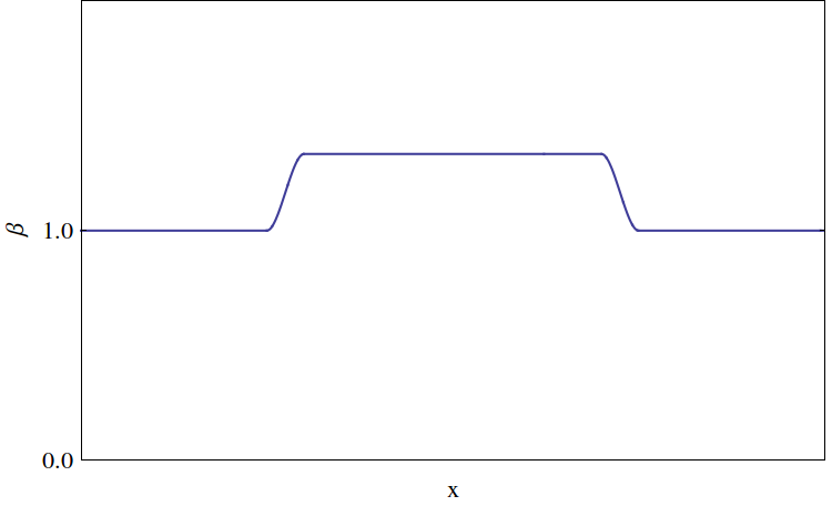
Metric (46) with conformal factor (3.8) is isometric to $q_{0}$ constructed by matching in Section 3. In the next step we introduce voids and overdensities by multiplying the conformal factor by a function $\chi_{1}$ which is equal to 1 outside all the voids $D_{i}$, but not equal inside, see Figure 9. For each void we introduce the function

$\displaystyle\beta_{i}(r)=\left\{\begin{array}[]{ll}C_{i}\,\frac{\phi_{0}(g_{i}r)}{\phi_{0}(r)}&\textrm{if }r\leq\widehat{R}_{i}\\ 1&\textrm{if }r>\widehat{R}_{i}\end{array}\right.,$

where $\widehat{R}_{i}$ is the radius of the void/overdensity pair in conformal coordinates and the constants $C_{i}$ and $g_{i}$ are functions of $M$, $\widehat{R}$, and $\widehat{R}_{i}$ which ensure that $\beta_{i}$ is continuous together with its first derivative across $r=\widehat{R}_{i}$ (this is always possible, although the exact expressions for them are quite complicated and irrelevant here), see Figure 9.

Let now $S_{i}$ denote a rotation of the spherical cap $C$ which takes its center $p$ to the center $p_{i}$ of the overdensity $D_{i}$. $S_{i}$ is only defined on a subset of $C$, but it can be uniquely extended to a proper conformal transformation $\Xi_{i}$ of the underlying flat metric. We can now lump together all $\beta_{i}$ functions into a single one, defined as their product:

$\displaystyle\chi_{1}=\prod_{i=1}^{n}\beta_{i}\circ\Xi_{i}.$

Now the conformal factor $\phi_{1}=\phi_{0}\chi_{1}$ substituted to (46) yields a metric isometric to $q_{1}$.

In order to construct functions $\chi_{2}$ and higher, yielding the next steps of the construction, we only need to scale down functions $\beta_{i}$ and place them correctly. Let $T_{i}$ be the rescaling $T_{i}:\textbf{R}^{3}\ni x^{k}\mapsto g_{i}\,x^{k}\in\textbf{R}^{3}$ with factor $g_{i}$ and let $F_{i}=\Xi_{i}\circ T_{i}$. $F_{i}$ maps $C$ into the appropriate smaller cap $C_{i}$. We now take

	$\displaystyle\chi_{N}$	$\displaystyle=$	$\displaystyle\prod_{i_{1},\dots,i_{N}}^{n}\beta_{i_{1}}\circ\Xi_{i_{1}}\circ F_{i_{2}}^{-1}\circ\cdots\circ F_{i_{N}}^{-1}$
	$\displaystyle\phi_{N}$	$\displaystyle=$	$\displaystyle\phi_{0}\,\chi_{1}\cdots\chi_{N}.$

Note that each of the $\chi_{k}$ is itself of the order of $1+O(\varepsilon)$ inside the overdense spheres of appropriate nesting level, so inside the smallest overdense spheres the conformal factor is of the order of $(1+O(\varepsilon))^{N}$. For a deeply nested structure ($N\approx\varepsilon^{-1}$) this means that in the vicinity of the smallest overdensities the conformal factor deviates significantly from $1$, see Figure 9. This means of course that the solution lies beyond the regime of validity of simple GR linearized around a flat solution, although the total volume of space where $\phi$ deviates significantly from 1 is rather small.

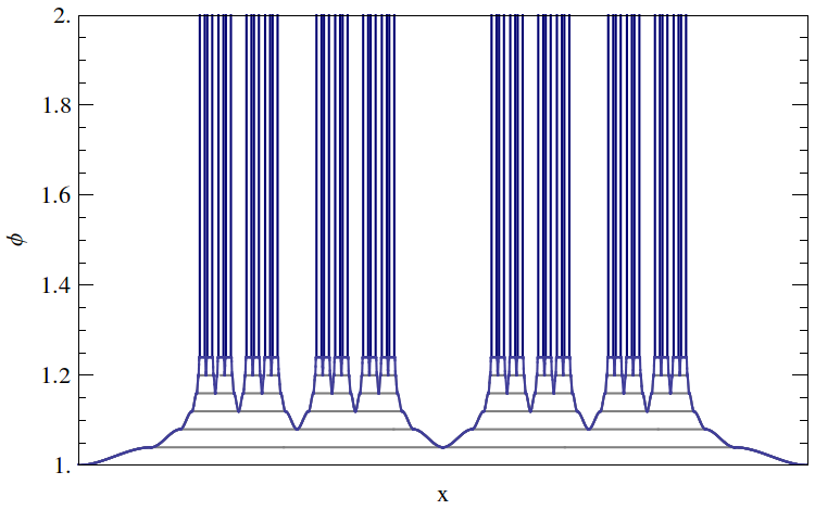
We arrive thus at the following conclusion: in the conformal gauge each single void/overdensity pair can be described by a small, quasi–Newtonian perturbation of the conformal factor, but if we try to extend this type of approach to the whole multiscale foam we note that it fails on the global level. The problem is that it is impossible to extend a conformal coordinate system up to the scale of the whole object without violating the smallness condition for the conformal factor. Such extension would be possible only if we somehow wiped out the finest structures in the matter distribution, i.e. adapt a coarse–graining approach to the problem, which will be discrussed in the next section. This problem with the conformal gauge has already been noted, see the paper by Buchert, Ellis and van Elst [12] in the memory of Jürgen Ehlers.

It is possible to embed the multiscale foam in a Swiss–cheese cosmological model. Consider a closed FLRW model at the moment of its largest expansion, with the spatial metric of the form of a 3–sphere of radius ${\cal R}$ given by (10). Let $\Lambda\ll 1$ be a small angle. We excise a densely packed (not necessary regular) lattice of caps of radius $\Lambda$ and fill them with multiscale foam balls with ADM mass $M=\frac{{\cal R}}{2}\sin^{3}\Lambda$ and area radius $R={\cal R}\sin\Lambda$. This way we obtain a cosmological solution $r_{N}$ with the metric tensor very close to the close FLRW model with dust, but with multiscale structure present throughout the universe, see Figure 10. More precisely, the metric $q_{S}$ from (10) is an excellent approximation of $r_{N}$ everywhere except the smallest and densest overdense regions.

Let us focus on its properties at the moment of the largest expansion and consider the relation between the cosmological parameters describing the matter content inferred from properties of the large scale averaged solution $q_{S}$ and average of the local energy density. The mass of any of the excised balls calculated with the averaged metric $q_{S}$ is obviously $M$. On the other hand the integral of the physical energy density with the physical volume form yields $M_{\textrm{tot}}$. As we have seen, these two values can be very different. Consequently in the presence of the hierarchy of nested overdensities and voids the average energy density inferred from the averaged metric $q_{S}$ may differ significantly from the average of energy density of $r_{N}$. In the language of [2] this means that a significant $00$ component of the backreaction tensor $t^{(0)}$ is present. This example shows that the presence of multiscale structure in cosmology may lead to accumulation of nonlinear effects of GR resulting in large backreaction terms in the effective FLRW equations.

Consider the uniform ball of dust $C$. Instead of solving the full equations we solve the first order approximation in $\varepsilon$, given by equation (6). We will work in dimensionless variables introduced in Section 2, although for the sake of clarity we will omit the tildes over them. We have

$\displaystyle\rho(x)=\left\{\begin{array}[]{ll}\frac{3}{4\pi}&\textrm{if }\|x\|\leq 1\\ 0&\textrm{otherwise}\end{array}\right.$

and for $\zeta$ we obtain

$\displaystyle\zeta(x)=\left\{\begin{array}[]{ll}\frac{1}{2}\left(\|x\|^{2}-3\right)&\textrm{if }\|x\|\leq 1\\ -\|x\|^{-1}&\textrm{otherwise}\end{array}\right.$

($\|\cdot\|$ denotes here the norm with respect to the Euclidean metric $\delta_{ij}$). Let us now introduce a void/overdensity pair centered at $p$, given by $x_{p}^{i}$ in our coordinate system. The new energy density $\widetilde{\rho}_{a}$ reads now

$\displaystyle\rho_{a}(x)=\left\{\begin{array}[]{ll}\sigma&\textrm{if }\|x-x_{p}\|\leq R_{\textrm{in}}\\ 0&\textrm{if }R_{\textrm{in}}<\|x-x_{p}\|\leq R_{\textrm{out}}\\ \rho(x)&\textrm{otherwise.}\end{array}\right.$

The conservation of the $ADM$ mass implies that

$\displaystyle\int\rho\,\textrm{d}^{3}x=\int\rho_{a}\,\textrm{d}^{3}x$

so

$\displaystyle\sigma=\frac{3R_{\textrm{out}}^{3}}{4\pi R_{\textrm{in}}^{3}}+O(\varepsilon).$

The self-similarity condition on the other hand implies that the compactness of $C$ and $C_{i}$ is the same:

$\displaystyle\varepsilon\sigma R_{\textrm{in}}^{2}=\varepsilon\rho R^{2}=\frac{3\varepsilon}{4\pi}+O(\varepsilon)$

(the last equality follows from the fact that in the dimensionless variables $R=1$). Taken together the equations above imply that

$\displaystyle R_{\textrm{in}}=R_{\textrm{out}}^{3}+O(\varepsilon).$

The new potential $\zeta_{a}$ reads

$\displaystyle\zeta_{a}(x)=\left\{\begin{array}[]{ll}\left(\frac{R_{\textrm{out}}}{R_{\textrm{in}}}\right)^{3}\frac{\|x-x_{p}\|^{2}}{2}+F_{1}&\textrm{if }\|x-x_{p}\|\leq R_{\textrm{in}}\\ -R_{\textrm{out}}^{3}\,\|x-x_{p}\|^{-1}+F_{2}&\textrm{if }R_{\textrm{in}}<\|x-x_{p}\|\leq R_{\textrm{out}}\\ \zeta(x)&\textrm{otherwise.}\\ \end{array}\right.,$

where

	$\displaystyle F_{1}$	$\displaystyle=$	$\displaystyle\frac{3}{2}\left(R_{\textrm{out}}^{2}-1-\frac{R_{\textrm{out}}^{3}}{R_{\textrm{in}}}\right)+x_{p}\cdot x+\frac{1}{2}\|x_{p}\|^{2}$
	$\displaystyle F_{2}$	$\displaystyle=$	$\displaystyle\frac{3}{2}\left(R_{\textrm{out}}^{2}-1\right)+x_{p}\cdot x+\frac{1}{2}\|x_{p}\|^{2}$

and the scalar product is again given by the metric $\delta_{ij}$. We can now evaluate the difference between the total mass before and after the introduction of the void: since the ADM mass does not change, we may use (8) to obtain

$\displaystyle M_{\textrm{tot,a}}-M_{\textrm{tot}}=-\frac{\varepsilon}{2}\int\left(\rho_{a}\zeta_{a}-\rho\zeta\right)\textrm{d}^{3}x.$

Unsurprisingly the difference is simply equal to the increase of the Newtonian binding energy due to compression of the matter from the void into a ball of smaller radius. In our case it reads

$\displaystyle M_{\textrm{tot,a}}-M_{\textrm{tot}}=\frac{3\varepsilon}{5}R_{\textrm{out}}^{3}\left(1-R_{\textrm{out}}^{2}\right)+O(\varepsilon^{2}).$

Since the volume fraction is

$\displaystyle\alpha_{i}=R_{\textrm{out}}^{-3}\left(1-\frac{9\varepsilon}{10}\left(1-R_{\textrm{out}}^{2}\right)\right)+O(\varepsilon^{2})$

(67)

we obtain

$\displaystyle M_{\textrm{tot,a}}-M_{\textrm{tot}}=\frac{3\varepsilon}{5}\alpha_{i}(1-\alpha_{i}^{2/3})+O(\varepsilon^{2}).$

Note that in the dimensionless variables the total mass is $M_{\textrm{tot}}=1-O(\varepsilon)$, so

$\displaystyle\delta_{i}=\frac{3\varepsilon}{5}\alpha_{i}(1-\alpha_{i}^{2/3})+O(\varepsilon^{2})$

and for $n$ non–overlapping void/overdensity pairs we can express the parameter $\delta$ as

$\displaystyle\delta=\frac{3\varepsilon}{5}\sum_{i=1}^{n}\alpha_{i}(1-\alpha_{i}^{2/3})+O(\varepsilon^{2}).$

(68)

It remains to express the rescaling coefficients $\gamma_{i}$ by $R_{\textrm{out}}$ and $\varepsilon$. This can be done by repeating the reasoning from Section 3.4: we note first that that $\gamma_{i}$ is given by the ratio of the masses of $C$ before we create the void/overdensity pair $M_{\textrm{tot}}(C)=1$ and the mass of $C_{i}$, i.e.

$\displaystyle\gamma_{i}=\frac{M_{\textrm{tot}}(C_{i})}{M_{\textrm{tot}}(C)}=\frac{\alpha_{i}\,M_{\textrm{tot}}(C)+\delta_{i}\,M_{\textrm{tot}}(C)}{M_{\textrm{tot}}(C)}=\alpha_{i}+\delta_{i}.$

This identity is true in all orders of expansion in $\varepsilon$. It follows that the summed up coefficients satisfy

$\displaystyle\gamma=\alpha+\delta,$

(69)

which, together with (67) and (68), provides a first order approximation for $\gamma$ in $\varepsilon$. We can now repeat the whole reasoning leading to equations (32) and (33) for $M_{\textrm{tot}}$ as a function of dimensionless $\gamma$ and $\delta$. Substituting the Taylor expansions (68), (67) and (69) to these equations yields the approximate expression for the mass deficit.

References

- [1] Clarkson C, Ellis G, Larena J and Obinna U 2011 Rep. Prog. Phys. 74 112901
- [2] Green S R and Wald R M 2014 (Preprint 1407.8084)
- [3] Green S R and Wald R M 2011 Phys.Rev. D83 084020 (Preprint 1011.4920)
- [4] Ishibashi A and Wald R M 2006 Classical and Quantum Gravity 23 235
- [5] Alécian E and Morsink S M 2004 The Astrophysical Journal 614 914
- [6] Wald R 2010 General Relativity (University of Chicago Press) chap 6
- [7] Misner C W, Thorne K S and Wheeler J A 1973 Gravitation chap 23, p 607
- [8] Boyd D W 1973 Canadian Journal of Mathematics 25 303–322
- [9] Boyd D W 1973 Mathematics of Computation 27
- [10] Borkovec M, de Paris W and Peikert R 1994 Fractals 2 521–526
- [11] Mandelbrot B B 1983 The Fractal Geometry of Nature (W.H. Freeman and Company)
- [12] Buchert T, Ellis G F and Elst H 2009 General Relativity and Gravitation 41 2017–2030
- [13] Horvath I, Hakkila J and Bagoly Z 2013 (Preprint 1311.1104)
- [14] Buchert T 2008 Gen.Rel.Grav. 40 467–527 (Preprint 0707.2153)
- [15] Ishibashi A and Wald R M 2006 Class.Quant.Grav. 23 235–250 (Preprint gr-qc/0509108)
- [16] Korzyński M 2014 Classical and Quantum Gravity 31 085002
- [17] Clifton T 2014 Class.Quant.Grav. 31 175010 (Preprint 1405.3197)
- [18] Isaacson R A 1968 Physical Review 166 1263
- [19] Isaacson R A 1968 Physical Review 166 1272
- [20] Burnett G A 1989 Journal of Mathematical Physics 30