跳到论文正文
W Papers独立论文阅读器 arXiv:1412.3847 论文正文 计算阅读时间 · 0%
引用这篇论文根据当前论文元数据生成,正式投稿前建议核对。


License: arXiv.org perpetual non-exclusive license
arXiv:1412.3847v1 [math-ph] 11 Dec 2014

Potentials of the Heun class: the triconfluent case

D. Batic Email: davide.batic@uwimona.edu.jm Affiliation: Department of Mathematics,
University of the West Indies, Kingston 6, Jamaica
   D. Mills-Howell Email: dominic.millz27@gmail.com Affiliation: Department of Mathematics,
University of the West Indies, Kingston 6, Jamaica
   M. Nowakowski Email: mnowakos@uniandes.edu.co Affiliation:  Departamento de Fisica,
Universidad de los Andes, Cra.1E No.18A-10, Bogota, Colombia
August 24, 2026
Abstract

Since the advent of quantum mechanics different approaches to find analytical solutions of the Schrödinger equation have been successfully developed. Here we follow and generalize the approach pioneered by Natanzon and others by which the Schrödinger equations can be transformed into another well-known equation for transcendental function (e.g., the hypergeometric equation). This sets a class of potentials for which this transformation is possible. Our generalization consists in finding potentials allowing the transformation of the Schrödinger equation into a triconfluent Heun equation. We find the energy eigenvalues of this class of potentials, the eigenfunction and the exact superpartners.

pacs
XXX

I Introduction

The study of exactly solvable Schrödinger equations can be traced back to the beginning of quantum mechanics. The earliest examples are represented by the harmonic oscillator, Coulomb, Morse, Pöschl-Teller, Eckart and Manning-Rosen potentials [1, 2, 3]. By looking closer at these examples one can start to conjecture that exact solvability of the Schrödinger equation depends on the fact that such an equation can be suitably reduced to the hypergeometric or the confluent hypergeometric equation. The problem of deriving the most general class of potentials such that the Schrödinger equation can be transformed into the hypergeometric equation has been solved by [4]. Furthermore, [5] studied solutions regular at infinity for the basic SUSY ladder of Hyperbolic Pöschl-Teller potentials that admit representations in terms of confluent Heun polynomials. [6] derived new classes of potentials such that the one-dimensional Schrödinger equation can be turned into the Heun equation and its confluent cases. The generalized Heun equation has been considered as well in [6]. Since the hypergeometric equation

y⁡(1−y)​d2​vd​y2+[c−(a+b+1)​y]​d​vd​y−a​b​v​(y)=0,y∈I⊂ℝy(1-y)\frac{d^{2}v}{dy^{2}}+\left[c-(a+b+1)y\right]\frac{dv}{dy}-abv(y)=0,\quad y\in I\subset\mathbb{R} (1)

with a,b,c∈ℝa,b,c\in\mathbb{R} is a special case of the Heun equation

d2​vd​y2+(γy+δy−1+ϵy−a)​d​vd​y+α​β​y−qy​(y−1)​(y−a)​v​(y)=0,y∈I⊂ℝ,\frac{d^{2}v}{dy^{2}}+\left(\frac{\gamma}{y}+\frac{\delta}{y-1}+\frac{\epsilon}{y-a}\right)\frac{dv}{dy}+\frac{\alpha\beta y-q}{y(y-1)(y-a)}v(y)=0,\quad y\in I\subset\mathbb{R}, (2)

whenever q=α​β​aq=\alpha\beta a and ϵ=0\epsilon=0, the potential classes obtained in [6] generalizes the Natanzon’s class. We start by reviewing the method developed by [7, 6] allowing the construction of the most general potential such that the Schrödinger equation can be reduced to the triconfluent Heun equation (5). Such a potential contains six free parameters.

II Reduction of the radial Schrödinger equation to a triconfluent Heun equation

We consider a quantum particle in a central field in three and two spatial dimensions, respectively. In the three dimensional case the behaviour of the particle is described by the Schrödinger equation (ℏ2=2​m=1\hbar^{2}=2m=1)

i​∂tΨ⁡(t,𝐫)=H​Ψ​(t,𝐫),H=−Δ+U⁡(r)i\partial_{t}\Psi(t,{\bf{r}})=H\Psi(t,{\bf{r}}),\quad H=-\Delta+U(r)

with Ψ∈L2​(ℝ3)\Psi\in L^{2}(\mathbb{R}^{3}). Here, Δ\Delta denotes the Laplacian. Since the Hamilton operator commutes with the angular momentum operator 𝐋=(Lx,Ly,Lz){\bf{L}}=(L_{x},L_{y},L_{z}), it is sufficient to solve the eigenvalue problem for HH, i.e. the time-dependent Schrödinger equation, on the subspace of L2​(ℝ3)L^{2}(\mathbb{R}^{3}) spanned by a basis of common eigenvectors of |𝐋2||{\bf{L}}^{2}| and LzL_{z}. Such a subspace is made of functions having the form Φℓ​m​(r,θ,ϕ)=Φ⁡(r)​Yℓ​m​(θ,ϕ)\Phi_{\ell m}(r,\theta,\phi)=\Phi(r)Y_{\ell m}(\theta,\phi) where Φ∈L2​(ℝ+,r2​d​r)\Phi\in L^{2}(\mathbb{R}_{+},r^{2}dr) and Yℓ​m​(θ,ϕ)Y_{\ell m}(\theta,\phi) denotes the spherical harmonics. In spherical coordinates the Laplace operator becomes

Δ=1r2∂rr2∂r−|𝐋2|r2.\Delta=\frac{1}{r^{2}}\partial_{r}r^{2}\partial_{r}-\frac{|{\bf{L}}^{2}|}{r^{2}}.

If Φℓ​m\Phi_{\ell m} is an eigenfunction of HH relative to the eigenvalue EE, then Φ\Phi must satisfy the radial Schrödinger equation [8]

[−(d2d​r2+2r​dd​r−ℓ⁡(ℓ+1)r2)+U⁡(r)]​Φ​(r)=E​Φ​(r).\left[-\left(\frac{d^{2}}{dr^{2}}+\frac{2}{r}\frac{d}{dr}-\frac{\ell(\ell+1)}{r^{2}}\right)+U(r)\right]\Phi(r)=E\Phi(r).

The above equation can be further simplified if we bring it to its canonical form by means of the transformation Φ⁡(r)=ψ⁡(r)/r\Phi(r)=\psi(r)/r with ψ∈L2​(ℝ+,r2​d​r)\psi\in L^{2}(\mathbb{R}_{+},r^{2}dr) and we obtain

d2​ψd​r2+[E−Ve​f​f​(r)]​ψ​(r)=0,Ve​f​f​(r)=ℓ⁡(ℓ+1)r2+U⁡(r).\frac{d^{2}\psi}{dr^{2}}+\left[E-V_{eff}(r)\right]\psi(r)=0,\quad V_{eff}(r)=\frac{\ell(\ell+1)}{r^{2}}+U(r). (3)

The region where the dynamics of the particle can take place is constrained to the half axis r>0r>0. Moreover, it will be assumed that the effective potential does not depend on the energy of the particle. Two-dimensional quantum systems appear in solid state physics in connection with the fractional quantum Hall effect [9] and high temperature superconductivity [10, 11, 12]. For the two-dimensional case we consider a system of two anyons [13], i.e. particles with fractional statistics, in a spherically-symmetric potential. The time-independent Schrödinger equation governing this system is [14, 15] (ℏ2=2​μ=1\hbar^{2}=2\mu=1 with μ\mu the reduced mass of the system)

[−(d2d​r2+1r​dd​r−ν2r2)+U⁡(r)]​Φ​(r)=E​Φ​(r),ν=m+θπ,\left[-\left(\frac{d^{2}}{dr^{2}}+\frac{1}{r}\frac{d}{dr}-\frac{\nu^{2}}{r^{2}}\right)+U(r)\right]\Phi(r)=E\Phi(r),\quad\nu=m+\frac{\theta}{\pi},

where θ\theta is the statistics parameter, m∈ℤm\in\mathbb{Z} is the azimuthal quantum number and r=|𝐫1−𝐫2|>0r=|{\bf{r}}_{1}-{\bf{r}}_{2}|>0 is the relative coordinate. Note that r≠0r\neq 0 to avoid that the two particles overlap. By means of the substitution Φ⁡(r)=ψ⁡(r)/r\Phi(r)=\psi(r)/\sqrt{r} we get formally the same Schrödinger equation as given by (3) with

Ve​f​f​(r)=ν2−14r2+U⁡(r).V_{eff}(r)=\frac{\nu^{2}-\frac{1}{4}}{r^{2}}+U(r). (4)

We want to construct the most general potential UU such that the radial Schrödinger equation (3) with effective potential given by (3) with ℓ=0\ell=0 or (4) with fixed ν\nu can be transformed into the triconfluent Heun equation [16]

d2​vd​ρ2+I⁡(ρ)​v​(ρ)=0,I⁡(ρ)=A0+A1​ρ+A2​ρ2−94​ρ4\frac{d^{2}v}{d\rho^{2}}+I(\rho)v(\rho)=0,\quad I(\rho)=A_{0}+A_{1}\rho+A_{2}\rho^{2}-\frac{9}{4}\rho^{4} (5)

with parameters A1,A2,A2∈ℝA_{1},A_{2},A_{2}\in\mathbb{R} and ρ∈Ω⊆ℝ\rho\in\Omega\subseteq\mathbb{R}. Note that (5) can be obtained by means of a confluence process of the singularities involved in the Heun equation. To appreciate the role of the TCH equation in physics, we refer to [17, 18, 19, 20] where this equation appears in the treatment of anharmonic oscillators in quantum mechanics. A short exposition of known results concerning anharmonic oscillators can be found in Ch. I of [21]. It is interesting to observe that the radial Schrödinger equation (3) reduces immediately to the above triconfluent Heun equation whenever

r=ρ,ψ=v,E=A0,ℓ=0,U⁡(r)=−A1​r−A2​r2+94​r4,r=\rho,\quad\psi=v,\quad E=A_{0},\quad\ell=0,\quad U(r)=-A_{1}r-A_{2}r^{2}+\frac{9}{4}r^{4},

i.e. UU is a quartic potential. In what follows we are interested in non trivial transformations of the dependent variable ψ\psi and the radial coordinate rr transforming (3) into (5). As in [6] we introduce the coordinate transformation ρ=ρ⁡(r)\rho=\rho(r) with r>0r>0 and (5) becomes

d2​vd​r2−ρ′′ρ′d​vd​r+(ρ′)2I(ρ(r))v(ρ(r))=0,′:=dd​r.\frac{d^{2}v}{dr^{2}}-\frac{\rho^{{}^{\prime\prime}}}{\rho^{{}^{\prime}}}\frac{dv}{dr}+(\rho^{{}^{\prime}})^{2}I(\rho(r))v(\rho(r))=0,\quad^{{}^{\prime}}:=\frac{d}{dr}.

The standard form of the above equation can be achieved by using the Liouvillle transformation

v⁡(ρ⁡(r))=exp​(12​∫ρ′′(r)ρ′(r)​𝑑r)​ψ​(r)=ρ′(r)​ψ​(r),v(\rho(r))=\mbox{exp}\left(\frac{1}{2}\int\frac{\rho^{{}^{\prime\prime}}(r)}{\rho^{{}^{\prime}}(r)}~dr\right)\psi(r)=\sqrt{\rho^{{}^{\prime}}(r)}\psi(r),

where we must require that

ρ′(r)>0\rho^{{}^{\prime}}(r)>0 (6)

on the interval (0,∞)(0,\infty), i.e. ρ\rho must be an increasing function of the variable rr. Hence, we end up with the linear ODE

d2​ψd​r2+J(r)ψ(r)=0,J(r)=(ρ′)2I(ρ(r))+12S(ρ).\frac{d^{2}\psi}{dr^{2}}+J(r)\psi(r)=0,\quad J(r)=(\rho^{{}^{\prime}})^{2}I(\rho(r))+\frac{1}{2}S(\rho). (7)

Here, S⁡(ρ)S(\rho) denotes the Schwarzian derivative of the coordinate transformation ρ\rho evaluated at rr and it is given by

S⁡(ρ)=ρ′′′ρ′−32​(ρ′′ρ′)2.S(\rho)=\frac{\rho^{{}^{\prime\prime\prime}}}{\rho^{{}^{\prime}}}-\frac{3}{2}\left(\frac{\rho^{{}^{\prime\prime}}}{\rho^{{}^{\prime}}}\right)^{2}.

It can be easily checked that solutions of (7) will be expressed in terms of the solutions of (5) according to

ψ⁡(r)=1ρ′(r)​v​(ρ⁡(r)).\psi(r)=\frac{1}{\sqrt{\rho^{{}^{\prime}}(r)}}v(\rho(r)).

Moreover, equation (7) will reduce to the radial Schrödinger equation (3) when J⁡(r)=E−Ve​f​f​(r)J(r)=E-V_{eff}(r). Therefore, the effective potential is completely determined by the Bose invariant II [22] and the Schwarzian derivative of the coordinate transformation. In order to be sure that the potential does not depend on the energy of the particle, we must require that

  • •

    the Bose invariant admits a decomposition of the form

    I⁡(ρ)=I0​(ρ)+E​I1​(ρ).I(\rho)=I_{0}(\rho)+EI_{1}(\rho). (8)

    According to Theorem IV.6 in [6], this will be the case if the parameters entering in the triconfluent Heun equation can be written as Ai=ai+E​biA_{i}=a_{i}+Eb_{i} with i=0,1,2i=0,1,2 and ai,bi∈ℝa_{i},b_{i}\in\mathbb{R} for any i=0,1,2i=0,1,2. Then, we have

    I0​(ρ)=a0+a1​ρ+a2​ρ2−94​ρ4,I1​(ρ)=b0+b1​ρ+b2​ρ2.I_{0}(\rho)=a_{0}+a_{1}\rho+a_{2}\rho^{2}-\frac{9}{4}\rho^{4},\quad I_{1}(\rho)=b_{0}+b_{1}\rho+b_{2}\rho^{2}.
  • •

    The coordinate transformation satisfies the differential equation

    (ρ′)2I1(ρ(r))=1.\left(\rho^{{}^{\prime}}\right)^{2}I_{1}(\rho(r))=1. (9)

    The condition expressed by (6) implies that we have to take the positive square root of (9), that is

    ρ′(r)=1I1​(ρ​(r)).\rho^{{}^{\prime}}(r)=\frac{1}{\sqrt{I_{1}(\rho(r))}}. (10)

With the help of (8) and (9) the effective potential can be written as

Ve​f​f​(r)=−I0​(ρ​(r))I1​(ρ​(r))−12​S​(ρ).V_{eff}(r)=-\frac{I_{0}(\rho(r))}{I_{1}(\rho(r))}-\frac{1}{2}S(\rho).

Rewriting the Schwarzian derivative in terms of I1I_{1} and its derivatives with respect to ρ\rho we obtain the most general form for the effective potential such that the radial Schrödinger equation (3) can be transformed into a triconfluent Heun equation, namely

Ve​f​f​(r)=−I0​(ρ​(r))I1​(ρ​(r))+4​I1​(ρ⁡(r))​I1¨​(ρ⁡(r))−5​I1˙2​(ρ⁡(r))16​I13​(ρ⁡(r)),˙:=dd​ρ.V_{eff}(r)=-\frac{I_{0}(\rho(r))}{I_{1}(\rho(r))}+\frac{4I_{1}(\rho(r))\ddot{I_{1}}(\rho(r))-5\dot{I_{1}}^{2}(\rho(r))}{16I_{1}^{3}(\rho(r))},\quad\dot{}:=\frac{d}{d\rho}. (11)

Replacing the corresponding expressions for I0I_{0} and I1I_{1} into (11) we can write the effective potential as

Ve​f​f​(r)=−4​a0+4​a1​ρ+4​a2​ρ2−9​ρ44​(b0+b1​ρ+b2​ρ2)−12​b22​ρ2+12​b1​b2​ρ+5​b12−8​b0​b216​(b0+b1​ρ+b2​ρ2)3,ρ=ρ⁡(r).V_{eff}(r)=-\frac{4a_{0}+4a_{1}\rho+4a_{2}\rho^{2}-9\rho^{4}}{4(b_{0}+b_{1}\rho+b_{2}\rho^{2})}-\frac{12b_{2}^{2}\rho^{2}+12b_{1}b_{2}\rho+5b_{1}^{2}-8b_{0}b_{2}}{16(b_{0}+b_{1}\rho+b_{2}\rho^{2})^{3}},\quad\rho=\rho(r). (12)

Note that (12) represents a class of potentials depending upon the six real parameters ai,bia_{i},b_{i} with i=0,1,2i=0,1,2. Concerning the solution of the differential equation governing the coordinate transformation we need to require that I1​(ρ​(r))>0I_{1}(\rho(r))>0 for r∈(0,∞)r\in(0,\infty). Let Δ=b12−4​b0​b2\Delta=b_{1}^{2}-4b_{0}b_{2}. We have the following cases

  1. 1.

    b0,b1,b2≠0b_{0},b_{1},b_{2}\neq 0 and b2>0b_{2}>0.

    1. (a)

      If Δ<0\Delta<0, the coordinate transformation ρ\rho maps the interval (0,∞)(0,\infty) of the radial variable into the whole real line. Using 2.2612.261 and 2.262​(1)2.262(1) in [23] we find that the solution of (10) can be written as

      r⁡(ρ)=12​(ρ+b12​b2)​I1−Δ8​b2​b2​arcsinh​(2​b2​ρ+b1−Δ).r(\rho)=\frac{1}{2}\left(\rho+\frac{b_{1}}{2b_{2}}\right)\sqrt{I_{1}}-\frac{\Delta}{8b_{2}\sqrt{b_{2}}}\mbox{arcsinh}{\left(\frac{2b_{2}\rho+b_{1}}{\sqrt{-\Delta}}\right)}.

      As ρ→∞\rho\to\infty we see that r≈(b2/2)​ρ2r\approx(\sqrt{b_{2}}/2)\rho^{2}.

    2. (b)

      Let Δ=0\Delta=0. Since b12>0b_{1}^{2}>0, b2>0b_{2}>0, and b12=4​b0​b2b_{1}^{2}=4b_{0}b_{2}, then b0>0b_{0}>0 and b1=±2​b0​b2b_{1}=\pm 2\sqrt{b_{0}b_{2}}. Hence, I1=(b2​ρ±b0)2I_{1}=(\sqrt{b_{2}}\rho\pm\sqrt{b_{0}})^{2} and equation (10) becomes

      ρ′(r)=1b2​ρ±b0,\rho^{{}^{\prime}}(r)=\frac{1}{\sqrt{b_{2}}\rho\pm\sqrt{b_{0}}},

      where the plus sign must be taken when b1>0b_{1}>0. Note that ρ′>0\rho^{{}^{\prime}}>0 whenever ρ>∓b0/b2\rho>\mp\sqrt{b_{0}/b_{2}} where the minus sign must be taken for b1>0b_{1}>0. Integrating the above equation we obtain

      r⁡(ρ)=b22​ρ2±b0​ρ.r(\rho)=\frac{\sqrt{b_{2}}}{2}\rho^{2}\pm\sqrt{b_{0}}\rho.

      The above equation is quadratic in ρ\rho and therefore we can solve it in order to express ρ\rho as a function of the radial variable. In the case b1>0b_{1}>0 and requiring that ρ\rho is an increasing function of the radial variable we find that

      ρ⁡(r)=−b0+b0+2​b2​rb2.\rho(r)=\frac{-\sqrt{b_{0}}+\sqrt{b_{0}+2\sqrt{b_{2}}r}}{\sqrt{b_{2}}}.

      In this case ρ\rho maps the interval (0,∞)(0,\infty) into itself and the condition ρ>−b0/b2\rho>-\sqrt{b_{0}/b_{2}} is automatically satisfied. If b1<0b_{1}<0, by a similar reasoning we find the solution

      ρ⁡(r)=b0+b0+2​b2​rb2.\rho(r)=\frac{\sqrt{b_{0}}+\sqrt{b_{0}+2\sqrt{b_{2}}r}}{\sqrt{b_{2}}}.

      The image of the interval (0,∞)(0,\infty) under the transformation ρ\rho is the interval (2​b0/b2,∞)(2\sqrt{b_{0}/b_{2}},\infty) and also in this case the condition ρ>b0/b2\rho>\sqrt{b_{0}/b_{2}} is satisfied. If b0=0b_{0}=0, then Δ=0\Delta=0 implies b1=0b_{1}=0 and ρ\rho is given by the expression

      ρ⁡(r)=2​rb2.\rho(r)=\sqrt{\frac{2r}{\sqrt{b_{2}}}}.
    3. (c)

      If Δ>0\Delta>0, then I1>0I_{1}>0 on the interval (−∞,ρ1)∪(ρ2,∞)(-\infty,\rho_{1})\cup(\rho_{2},\infty) where ρ1\rho_{1} and ρ2\rho_{2} denote the roots of I1I_{1}. In this case we can express the radial variable in terms of ρ\rho as

      r⁡(ρ)=12​(ρ+b12​b2)​I1−Δ8​b2​b2​ln⁡(2​b2​I1+2​b2​ρ+b1).r(\rho)=\frac{1}{2}\left(\rho+\frac{b_{1}}{2b_{2}}\right)\sqrt{I_{1}}-\frac{\Delta}{8b_{2}\sqrt{b_{2}}}\ln{\left(2\sqrt{b_{2}I_{1}}+2b_{2}\rho+b_{1}\right)}.
  2. 2.

    b0,b1,b2≠0b_{0},b_{1},b_{2}\neq 0 and b2<0b_{2}<0. In this case only if Δ>0\Delta>0 we can make I1>0I_{1}>0 on an open interval (ρ1,ρ2)(\rho_{1},\rho_{2}) where ρ1\rho_{1} and ρ2\rho_{2} denote the roots of I1I_{1}. Employing 2.2612.261 and 2.262​(1)2.262(1) in [23] yield

    r⁡(ρ)=12​(ρ+b12​b2)​I1+Δ8​b2​−b2​arcsin​(2​b2​ρ+b1Δ).r(\rho)=\frac{1}{2}\left(\rho+\frac{b_{1}}{2b_{2}}\right)\sqrt{I_{1}}+\frac{\Delta}{8b_{2}\sqrt{-b_{2}}}\mbox{arcsin}\left(\frac{2b_{2}\rho+b_{1}}{\sqrt{\Delta}}\right).
  3. 3.

    If b2=0b_{2}=0 and b1≠0b_{1}\neq 0, then I1​(ρ)=b1​ρ+b0I_{1}(\rho)=b_{1}\rho+b_{0} and we must require that ρ>−b0/b1\rho>-b_{0}/b_{1}. The solution of the ODE governing the coordinate transformation is

    r⁡(ρ)=23​b1​(b1​ρ+b0)3/2.r(\rho)=\frac{2}{3b_{1}}(b_{1}\rho+b_{0})^{3/2}.

    Moreover, we can express ρ\rho in terms of the radial coordinate as

    ρ⁡(r)=−b0b1+1b1​(3​b1​r2)2/3.\rho(r)=-\frac{b_{0}}{b_{1}}+\frac{1}{b_{1}}\left(\frac{3b_{1}r}{2}\right)^{2/3}.

    We can observe that ρ\rho is an increasing function of rr and it maps the interval (0,∞)(0,\infty) to (−b0/b1,∞)(-b_{0}/b_{1},\infty). If b0=0b_{0}=0 the above expression simplifies to

    ρ(r)=(32)2/3b1−1/3r2/3.\rho(r)=\left(\frac{3}{2}\right)^{2/3}b_{1}^{-1/3}r^{2/3}.

III Analysis of the potentials

We analyze those potentials arising from the cases when the coordinate transformation ρ\rho can be written as an explicit function of the real variable rr.

III.1 The case Δ=0\Delta=0, and b0,b1,b2>0b_{0},b_{1},b_{2}>0

It is straightforward to verify that I1=b0+2​b2​rI_{1}=b_{0}+2\sqrt{b_{2}}r and the effective potential can be written as

V1​(r)=c0+c1b0+2​b2​r+c2b0+2​b2​r+c3(b0+2​b2​r)2+c4​b0+2​b2​r+c5​rV_{1}(r)=c_{0}+\frac{c_{1}}{\sqrt{b_{0}+2\sqrt{b_{2}}r}}+\frac{c_{2}}{b_{0}+2\sqrt{b_{2}}r}+\frac{c_{3}}{(b_{0}+2\sqrt{b_{2}}r)^{2}}+c_{4}\sqrt{b_{0}+2\sqrt{b_{2}}r}+c_{5}r (13)

with

c0=63​b04​b22−a2b2,c1=2​a2​b0b2−a1b2−9​b0​b0b22,c2=−a0+a1​b0b2+9​b024​b22−a2​b0b2,c_{0}=\frac{63b_{0}}{4b_{2}^{2}}-\frac{a_{2}}{b_{2}},\quad c_{1}=\frac{2a_{2}\sqrt{b_{0}}}{b_{2}}-\frac{a_{1}}{\sqrt{b_{2}}}-\frac{9b_{0}\sqrt{b_{0}}}{b_{2}^{2}},\quad c_{2}=-a_{0}+\frac{a_{1}\sqrt{b_{0}}}{\sqrt{b_{2}}}+\frac{9b_{0}^{2}}{4b_{2}^{2}}-\frac{a_{2}b_{0}}{b_{2}},
c3=−34​b2,c4=−9​b0b22,c5=92​b2​b2c_{3}=-\frac{3}{4}b_{2},\quad c_{4}=-\frac{9\sqrt{b_{0}}}{b_{2}^{2}},\quad c_{5}=\frac{9}{2b_{2}\sqrt{b_{2}}}

Note that c0=c1=c2=0c_{0}=c_{1}=c_{2}=0 if we choose

a0=9​(b0b2)2,a1=452​(b0b2)3/2,a2=63​b04​b2.a_{0}=9\left(\frac{b_{0}}{b_{2}}\right)^{2},\quad a_{1}=\frac{45}{2}\left(\frac{b_{0}}{b_{2}}\right)^{3/2},\quad a_{2}=\frac{63b_{0}}{4b_{2}}.

and the corresponding effective potential will depend only on the parameters b0b_{0} and b2b_{2}. We observe that

  1. 1.

    Since r>0r>0 and b0>0b_{0}>0, it follows that the denominators appearing in (13) can never vanish and therefore the potential is never singular on the open interval (0,∞)(0,\infty).

  2. 2.

    If r=0r=0 the potential is finite there while asymptotically for r→∞r\to\infty it grows linearly as

    V1​(r)≈9​r2​b2​b2.V_{1}(r)\approx\frac{9r}{2b_{2}\sqrt{b_{2}}}.
  3. 3.

    There are choices of the parameters such that V1V_{1} has at least a global minimum on the positive real line. See Fig. 1.

    Refer to caption
    Figure 1: Behaviour of the potential (13) for different choices of the parameters.

The study of the critical points of this potential leads to a polynomial equation of degree eight. Applying Descartes’ rule of signs we find that the potential (13) has four, two, or no positive critical points whenever c1c_{1} and c3c_{3} are negative and c2c_{2} is positive; three or one positive critical point if c1<0c_{1}<0 and c2,c3>0c_{2},c_{3}>0, and only one positive critical point if c1c_{1}, c2c_{2}, and c3c_{3} are positive. For other choices of the signs of the coefficients c1c_{1}, c2c_{2}, and c3c_{3} there are two or no positive critical point.

III.2 The case Δ=0\Delta=0, b0,b2>0b_{0},b_{2}>0, and b1<0b_{1}<0

The function I1I_{1} is formally given as in the previous case and the effective potential has the same form as (13) with coefficients d0,⋯,d5d_{0},\cdots,d_{5} given by

d0=c0,d1=−2​a2​b0b2−a1b2+9​b0​b0b22,d2=a0−a1​b0b2+9​b024​b22−a2​b0b2,d3=c3,d4=−c4,d5=c5.d_{0}=c_{0},\quad d_{1}=-\frac{2a_{2}\sqrt{b_{0}}}{b_{2}}-\frac{a_{1}}{\sqrt{b_{2}}}+\frac{9b_{0}\sqrt{b_{0}}}{b_{2}^{2}},\quad d_{2}=a_{0}-\frac{a_{1}\sqrt{b_{0}}}{\sqrt{b_{2}}}+\frac{9b_{0}^{2}}{4b_{2}^{2}}-\frac{a_{2}b_{0}}{b_{2}},\quad d_{3}=c_{3},\quad d_{4}=-c_{4},\quad d_{5}=c_{5}.

Note that d0=d1=d2=0d_{0}=d_{1}=d_{2}=0 if we choose

a0=−36​(b0b2)2,a1=−452​(b0b2)3/2,a2=63​b04​b2.a_{0}=-36\left(\frac{b_{0}}{b_{2}}\right)^{2},\quad a_{1}=-\frac{45}{2}\left(\frac{b_{0}}{b_{2}}\right)^{3/2},\quad a_{2}=\frac{63b_{0}}{4b_{2}}.

We observe that

  1. 1.

    Since r>0r>0 and b0>0b_{0}>0, it follows that I1I_{1} can never vanish and therefore the potential is never singular.

  2. 2.

    The potential is finite at r=0r=0 while asymptotically for r→∞r\to\infty it grows linearly as (13).

  3. 3.

    There are again choices of the parameters such that the potential has at least one minimum.

III.3 The case Δ=0\Delta=0, b2>0b_{2}>0, and b0=b1=0b_{0}=b_{1}=0

The potential takes the form

V3​(r)=e0+e1r+e2r+e3r2+e4​rV_{3}(r)=e_{0}+\frac{e_{1}}{\sqrt{r}}+\frac{e_{2}}{r}+\frac{e_{3}}{r^{2}}+e_{4}r (14)

where

e0=−a2b2,e1=−a12​b23/4,e2=−a02​b2,e3=−316,e4=c5.e_{0}=-\frac{a_{2}}{b_{2}},\quad e_{1}=-\frac{a_{1}}{\sqrt{2}b_{2}^{3/4}},\quad e_{2}=-\frac{a_{0}}{2\sqrt{b_{2}}},\quad e_{3}=-\frac{3}{16},\quad e_{4}=c_{5}.

Note that it becomes singular at r=0r=0 and asymptotically at infinity it behaves as (13). There are choices of the parameters such that this potential has a maximum very close to r=0r=0 and a minimum. See Fig. 2.

Refer to caption
Figure 2: Behaviour of the potential for the case Δ=0\Delta=0, b0,b2>0b_{0},b_{2}>0, and b1<0b_{1}<0.

The potential (14) is singular at r=0r=0 and it grows linearly for r→∞r\to\infty. We have choices of the parameters such that the potential exhibits maxima and minima. If we make the substitution r=τ2r=\tau^{2}, the critical points of the potential (14) must satisfy the sextic equation

2​e4​τ6−e1​τ3−2​e2​τ2−4​e3=0.2e_{4}\tau^{6}-e_{1}\tau^{3}-2e_{2}\tau^{2}-4e_{3}=0. (15)

If a0a_{0} and a1a_{1} are both positive, there is no change of sign in (15) and Descartes’ rule of signs implies that the sextic equation will not have any positive real root, and hence the potential has no extrema. For all other choices of the signs of the coefficients a0a_{0}, and a1a_{1}, there are only two sign changes in (15) and hence the potential will admit two positive critical points or none. For a complete root classification of a sextic equation we refer to [24].

III.4 The case b2=0b_{2}=0

It can be easily checked that I1​(r)=(3​b1​r/2)2/3I_{1}(r)=(3b_{1}r/2)^{2/3} and the potential can be written as

V4​(r)=v0+v1r2/3+v2r2+v3​r2/3+v4​r4/3+v5​r2V_{4}(r)=v_{0}+\frac{v_{1}}{r^{2/3}}+\frac{v_{2}}{r^{2}}+v_{3}r^{2/3}+v_{4}r^{4/3}+v_{5}r^{2} (16)

with

v0=−a1b1+2​a2​b0b12−9​b03b14,v1=(23​b1)2/3​(a1​b0b1−a0−a2​b02b12+9​b044​b14),v2=−536,v_{0}=-\frac{a_{1}}{b_{1}}+\frac{2a_{2}b_{0}}{b_{1}^{2}}-\frac{9b_{0}^{3}}{b_{1}^{4}},\quad v_{1}=\left(\frac{2}{3b_{1}}\right)^{2/3}\left(\frac{a_{1}b_{0}}{b_{1}}-a_{0}-\frac{a_{2}b_{0}^{2}}{b_{1}^{2}}+\frac{9b_{0}^{4}}{4b_{1}^{4}}\right),\quad v_{2}=-\frac{5}{36},
v3=1b12/3​(23​b1)2/3​[272​(b0b1)2−a2],v4=−310/3​b024/3​b18/3,v5=8116​b12.v_{3}=\frac{1}{b_{1}^{2/3}}\left(\frac{2}{3b_{1}}\right)^{2/3}\left[\frac{27}{2}\left(\frac{b_{0}}{b_{1}}\right)^{2}-a_{2}\right],\quad v_{4}=-\frac{3^{10/3}b_{0}}{2^{4/3}b_{1}^{8/3}},\quad v_{5}=\frac{81}{16b_{1}^{2}}.

We can set v0=v1=v3=0v_{0}=v_{1}=v_{3}=0 if we choose

a0=274​(b0b1)4,a1=18​(b0b1)3,a2=272​(b0b1)2.a_{0}=\frac{27}{4}\left(\frac{b_{0}}{b_{1}}\right)^{4},\quad a_{1}=18\left(\frac{b_{0}}{b_{1}}\right)^{3},\quad a_{2}=\frac{27}{2}\left(\frac{b_{0}}{b_{1}}\right)^{2}.

The potential (16) is singular at r=0r=0 and it grows quadratically for r→∞r\to\infty. We have choices of the parameters such that the potential exhibits maxima and minima. If we make the substitution r=τ3/2r=\tau^{3/2}, it is not difficult to verify that the critical points of the potential (16) must satisfy the sextic equation

3​v5​τ6+2​v4​τ5+v3​τ4−v1​τ2−3​v2=0.3v_{5}\tau^{6}+2v_{4}\tau^{5}+v_{3}\tau^{4}-v_{1}\tau^{2}-3v_{2}=0. (17)

If v1<0v_{1}<0 and v3,v4>0v_{3},v_{4}>0, we do not have any change of sign in (17) and Descartes’ rule of signs implies that the sextic equation will not have any positive real root, and therefore the potential has no extrema. If v1,v2>0v_{1},v_{2}>0 and v4<0v_{4}<0, there are four changes of sign and the potential may have four, two or no positive critical point. For all other choices of the signs of the coefficients v1v_{1}, v3v_{3}, and v4v_{4} there are only two sign changes in (17) and hence the potential will admit two positive critical points or none. In the subcase b2=b0=0b_{2}=b_{0}=0 the potential (16) simplifies to

V5​(r)=u0+u1r2/3+u2r2+u3​r2/3+u4​r2V_{5}(r)=u_{0}+\frac{u_{1}}{r^{2/3}}+\frac{u_{2}}{r^{2}}+u_{3}r^{2/3}+u_{4}r^{2} (18)

where

u0=−a1b1,u1=−a0​49​b123,u2=v2,u3=−a2​49​b143,u4=8116​b12.u_{0}=-\frac{a_{1}}{b_{1}},\quad u_{1}=-a_{0}\sqrt[3]{\frac{4}{9b_{1}^{2}}},\quad u_{2}=v_{2},\quad u_{3}=-a_{2}\sqrt[3]{\frac{4}{9b_{1}^{4}}},\quad u_{4}=\frac{81}{16b_{1}^{2}}.
Refer to caption
Figure 3: Behaviour of the potential (16) for different values of the parameters.

If we make the substitution r=τ3/4r=\tau^{3/4}, it is not difficult to verify that the critical points of the potential (18) must satisfy the cubic equation

3​u4​τ3+u3​τ2−u1​τ−3​u2=0.3u_{4}\tau^{3}+u_{3}\tau^{2}-u_{1}\tau-3u_{2}=0. (19)

If a2<0a_{2}<0 and a0>0a_{0}>0, we do not have any change of sign in (19) and Descartes’ rule of signs implies that the cubic equation will not have any positive real root. Hence, the potential has no positive extrema. For any other choice of the signs of the parameters a2a_{2} and a1a_{1}, we will always have two sign changes in (19) and therefore the potential will admit two positive critical points or none.

IV Solutions of the radial Schrödinger equation

We study the behaviour of the solutions of the radial Schrödinger equation for the general class of potentials (12) and for the potentials discussed in the previous section. First of all, by means of (10) the solution of the radial Schrödinger equation can be written as

ψ⁡(r)=b0+b1​ρ+b2​ρ24​v​(ρ),\psi(r)=\sqrt[4]{b_{0}+b_{1}\rho+b_{2}\rho^{2}}v(\rho),

where ρ=ρ⁡(r)\rho=\rho(r) and vv is a solution of the triconfluent Heun equation (5). It is in general convenient to bring (5) into its canonical form [16] with the help of the substitution

v⁡(ρ)=eA23​ρ−ρ32​y​(ρ),v(\rho)=e^{\frac{A_{2}}{3}\rho-\frac{\rho^{3}}{2}}y(\rho),

where the unknown function yy must satisfy the equation

d2​yd​ρ2−(γ+3​ρ2)​d​yd​ρ+[α+(β−3)​ρ]=0\frac{d^{2}y}{d\rho^{2}}-(\gamma+3\rho^{2})\frac{dy}{d\rho}+[\alpha+(\beta-3)\rho]=0 (20)

with

α=A0+A229,β=A1,γ=−23​A2.\alpha=A_{0}+\frac{A_{2}^{2}}{9},\quad\beta=A_{1},\quad\gamma=-\frac{2}{3}A_{2}. (21)

Hence, the general solution of the radial Schrödinger equation can be cast in the form

ψ⁡(r)=b0+b1​ρ+b2​ρ24​eA23​ρ−ρ32​y​(ρ).\psi(r)=\sqrt[4]{b_{0}+b_{1}\rho+b_{2}\rho^{2}}e^{\frac{A_{2}}{3}\rho-\frac{\rho^{3}}{2}}y(\rho). (22)

Note that the function multiplying yy in (22) decays exponentially in rr as r→+∞r\to+\infty because in the case b0,b1,b2≠0b_{0},b_{1},b_{2}\neq 0 we have

ρ⁡(r)≈{2​rb2if b2>0ρ2+1|b2|​(ρ2−ρ1)3​(3​r2)2/3if b2<0.\rho(r)\approx\left\{\begin{array}[]{ll}\sqrt{\frac{2r}{\sqrt{b_{2}}}}&\mbox{if $b_{2}>0$}\\ \rho_{2}+\frac{1}{\sqrt[3]{|b_{2}|(\rho_{2}-\rho_{1})}}\left(\frac{3r}{2}\right)^{2/3}&\mbox{if $b_{2}<0$}.\end{array}\right.

with ρ1\rho_{1} and ρ2\rho_{2} denoting the roots of the quadratic polynomial I1I_{1} introduced in Section II whereas if b2=0b_{2}=0 and b1≠0b_{1}\neq 0 we get

ρ⁡(r)≈1b1​(3​b1​r2)2/3.\rho(r)\approx\frac{1}{b_{1}}\left(\frac{3b_{1}r}{2}\right)^{2/3}.

Since equation (5) has no finite singular points, we can construct Taylor series for the solutions of the triconfluent Heun equation by adopting the method outlined in [16]. We first rewrite (20) in terms of the Euler operator δ=ρ​d/d​ρ\delta=\rho d/d\rho as

δ2​y−(1+γ​ρ+3​ρ3)​δ​y+(β−3)​ρ3​y=0.\delta^{2}y-(1+\gamma\rho+3\rho^{3})\delta y+(\beta-3)\rho^{3}y=0.

Observing that ρn\rho^{n} with n∈ℕn\in\mathbb{N} are eigenfunctions of the Euler operator, one finds the following two linearly independent solutions, namely

T1​(α,β,γ,ρ)=∑n=0∞en​(α,β,γ)​ρn,T2​(α,β,γ,ρ)=∑n=0∞sn​(α,β,γ)​ρn+1T_{1}(\alpha,\beta,\gamma;\rho)=\sum_{n=0}^{\infty}e_{n}(\alpha,\beta,\gamma)\rho^{n},\quad T_{2}(\alpha,\beta,\gamma;\rho)=\sum_{n=0}^{\infty}s_{n}(\alpha,\beta,\gamma)\rho^{n+1} (23)

with

e0​(α,β,γ)=1,e1​(α,β,γ)=0,e2​(α,β,γ)=−α2,e_{0}(\alpha,\beta,\gamma)=1,\quad e_{1}(\alpha,\beta,\gamma)=0,\quad e_{2}(\alpha,\beta,\gamma)=-\frac{\alpha}{2},
en​(α,β,γ)=(n−1)​γ​en−1​(α,β,γ)−α​en−2​(α,β,γ)−(β+6−3​n)​en−3​(α,β,γ)n⁡(n−1),n≥3e_{n}(\alpha,\beta,\gamma)=\frac{(n-1)\gamma e_{n-1}(\alpha,\beta,\gamma)-\alpha e_{n-2}(\alpha,\beta,\gamma)-(\beta+6-3n)e_{n-3}(\alpha,\beta,\gamma)}{n(n-1)},\quad n\geq 3

and

s0​(α,β,γ)=1,s1​(α,β,γ)=γ2,s2​(α,β,γ)=γ2−α6,s_{0}(\alpha,\beta,\gamma)=1,\quad s_{1}(\alpha,\beta,\gamma)=\frac{\gamma}{2},\quad s_{2}(\alpha,\beta,\gamma)=\frac{\gamma^{2}-\alpha}{6},
sn​(α,β,γ)=n​γ​sn−1​(α,β,γ)−α​sn−2​(α,β,γ)−(β+3−3​n)​sn−3​(α,β,γ)n⁡(n+1),n≥3.s_{n}(\alpha,\beta,\gamma)=\frac{n\gamma s_{n-1}(\alpha,\beta,\gamma)-\alpha s_{n-2}(\alpha,\beta,\gamma)-(\beta+3-3n)s_{n-3}(\alpha,\beta,\gamma)}{n(n+1)},\quad n\geq 3.

We will refer to (23) as the general solution to contrast it with the polynomial one which will be discussed below. Worth mentioning is also the convergence of (23) as shown in [16].

In order to find polynomial solutions of (20) we start AGAIN by assuming a power solution of the form

y⁡(ρ)=∑n=0∞wn​ρn.y(\rho)=\sum_{n=0}^{\infty}w_{n}\rho^{n}. (24)

Substituting (24) into (20) we obtain the following recurrence relation for the coefficients wnw_{n}

(β−3​n)​wn−1+α​wn−γ⁡(n+1)​wn+1+(n+1)​(n+2)​wn+2=0(\beta-3n)w_{n-1}+\alpha w_{n}-\gamma(n+1)w_{n+1}+(n+1)(n+2)w_{n+2}=0 (25)

which holds for all n≥0n\geq 0 provided that w−1=0w_{-1}=0. The above recursion relation is the same as the recursion relation for ene_{n} (see above) with a shift for nn. In order to have a polynomial solution of degree NN we require that wn=0w_{n}=0 for all n>Nn>N. Moreover, for n=N+1n=N+1 the recurrence relation above gives the condition β=3​(N+1)\beta=3(N+1). Taking into account that β=a1+b1​E\beta=a_{1}+b_{1}E, such a condition gives the energy eigenvalue

EN=3​(N+1)−a1b1,b1≠0E_{N}=\frac{3(N+1)-a_{1}}{b_{1}},\quad b_{1}\neq 0

with N=0,1,2,⋯N=0,1,2,\cdots. Furthermore, for 0≤n≤N0\leq n\leq N the recursion formula (25) generates a system of N+1N+1 homogenous linear equations for the coefficients w0,w1,⋯,wNw_{0},w_{1},\cdots,w_{N}. This system admits a non-trivial solution if and only if the determinant of the (N×1)×(N×1)(N\times 1)\times(N\times 1) matrix

DN+1=(α−γ200⋯03​Nα−2​γ2⋅30⋯03​(N−1)α−3​γ3⋅4⋯⋱3⋅3α−(N−1)​γN⁡(N−1)03⋅2α−N​γ0⋯003⋅1α)D_{N+1}=\begin{pmatrix}\alpha&-\gamma&2&0&0&\cdots&&&&0\\ 3N&\alpha&-2\gamma&2\cdot 3&0&\cdots&&&&\\ 0&3(N-1)&\alpha&-3\gamma&3\cdot 4&\cdots&&&&\\ \vdots&\vdots&\vdots&\vdots&\vdots&\ddots&&&&\vdots\\ &&&&&&3\cdot 3&\alpha&-(N-1)\gamma&N(N-1)\\ &&&&&&0&3\cdot 2&\alpha&-N\gamma\\ 0&&&&&\cdots&0&0&3\cdot 1&\alpha\end{pmatrix}

does not vanish. The first polynomials are given by

  • •

    N=0N=0: β=3\beta=3, α=0\alpha=0 and p0​(ρ)=1p_{0}(\rho)=1;

  • •

    N=1N=1: β=6\beta=6, α2+3​γ=0\alpha^{2}+3\gamma=0 and p1​(ρ)=ρ−α/3p_{1}(\rho)=\rho-\alpha/3;

  • •

    N=2N=2: β=9\beta=9, α3+12​α​γ+36=0\alpha^{3}+12\alpha\gamma+36=0 and

    p2​(ρ)=ρ2−α3​ρ+α236−1α;p_{2}(\rho)=\rho^{2}-\frac{\alpha}{3}\rho+\frac{\alpha^{2}}{36}-\frac{1}{\alpha};
  • •

    N=3N=3: β=12\beta=12, α4+30​α2​γ+216​α+81​γ2=0\alpha^{4}+30\alpha^{2}\gamma+216\alpha+81\gamma^{2}=0 and

    p3​(ρ)=ρ3−α3​ρ2+(γ2+α218)​ρ−α3162−754​α​γ−23;p_{3}(\rho)=\rho^{3}-\frac{\alpha}{3}\rho^{2}+\left(\frac{\gamma}{2}+\frac{\alpha^{2}}{18}\right)\rho-\frac{\alpha^{3}}{162}-\frac{7}{54}\alpha\gamma-\frac{2}{3};
  • •

    N=4N=4: β=15\beta=15, α5+60​α3​γ+756​α2+576​α​γ2+5184​γ=0\alpha^{5}+60\alpha^{3}\gamma+756\alpha^{2}+576\alpha\gamma^{2}+5184\gamma=0 and

    p4​(ρ)=ρ4−α3​ρ3+(α218+23​γ)​ρ2−(α3162+527​α​γ+43)​ρ+α41944+281​α2​γ+518​α+γ29.p_{4}(\rho)=\rho^{4}-\frac{\alpha}{3}\rho^{3}+\left(\frac{\alpha^{2}}{18}+\frac{2}{3}\gamma\right)\rho^{2}-\left(\frac{\alpha^{3}}{162}+\frac{5}{27}\alpha\gamma+\frac{4}{3}\right)\rho+\frac{\alpha^{4}}{1944}+\frac{2}{81}\alpha^{2}\gamma+\frac{5}{18}\alpha+\frac{\gamma^{2}}{9}.

Note that the above list extends the one given in [16]. The special case b1=0=b2b_{1}=0=b_{2} and b0=1b_{0}=1 and in particular the boundary value problem

−d2​vd​ρ2+P⁡(ρ)​v=E​v,v⁡(−∞)=v⁡(+∞)=0,P⁡(ρ)=94​ρ4−a2​ρ2−a1​ρ−a0-\frac{d^{2}v}{d\rho^{2}}+P(\rho)v=Ev,\quad v(-\infty)=v(+\infty)=0,\quad P(\rho)=\frac{9}{4}\rho^{4}-a_{2}\rho^{2}-a_{1}\rho-a_{0} (26)

has been considered by [25]. Note that the boundary condition is equivalent to the requirement v∈L2​(ℝ)v\in L^{2}(\mathbb{R}). According to [26, 27] the spectrum of the above problem is discrete, all eigenvalues are real and simple and they can be arranged into an increasing sequence E0<E1<⋯E_{0}<E_{1}<\cdots. Moreover, for n→∞n\to\infty the asymptotic behaviour of the eigenvalues is [25]

En≈[4​π​n2​B​(3/2,1/4)]4/3=[3​Γ2​(3/4)2​π​n]4/3,E_{n}\approx\left[\frac{4\pi n}{2B(3/2,1/4)}\right]^{4/3}=\left[\frac{3\Gamma^{2}(3/4)}{\sqrt{2\pi}}n\right]^{4/3},

where BB denotes the Euler function. Furthermore, all non-real zeros of the eigenfunctions of the problem (26) belong to the imaginary axis (see Theorem 1 in [28]).

We conclude this section by deriving a formula for the solution of the recurrence relation (25). By shifting the index according to the prescription n→n+1n\to n+1 we can rewrite (25) as a third order homogeneous linear difference equation

wn+3=−π1​(n,γ)​wn+2−π2​(n,α)​wn+1−π3​(n,β)​wnw_{n+3}=-\pi_{1}(n,\gamma)w_{n+2}-\pi_{2}(n,\alpha)w_{n+1}-\pi_{3}(n,\beta)w_{n} (27)

with n≥−2n\geq-2 and

π1​(n,γ)=−γn+3,π2​(n,α)=α(n+2)​(n+3),π3​(n,β)=β−3​(n+1)(n+2)​(n+3),w−2=w−1=0.\pi_{1}(n,\gamma)=-\frac{\gamma}{n+3},\quad\pi_{2}(n,\alpha)=\frac{\alpha}{(n+2)(n+3)},\quad\pi_{3}(n,\beta)=\frac{\beta-3(n+1)}{(n+2)(n+3)},\quad w_{-2}=w_{-1}=0.

By letting n=0n=0 we obtain w3w_{3} in terms of w2,w1w_{2},w_{1}, and w0w_{0}, namely

w3=γ3​w2−α2⋅3​w1−β−32⋅3​w0.w_{3}=\frac{\gamma}{3}w_{2}-\frac{\alpha}{2\cdot 3}w_{1}-\frac{\beta-3}{2\cdot 3}w_{0}.

Furthermore, for n=−2n=-2 and n=−1n=-1 we get, respectively

w1=γ​w0,w2=12​(γ2−α)​w0w_{1}=\gamma w_{0},\quad w_{2}=\frac{1}{2}(\gamma^{2}-\alpha)w_{0}

from which it follows that

w3=13!​[γ3−2​α​γ−(β−3)]​w0,w4=14!​[γ4−3​α​γ2+α2−3​γ​(β−5)]​w0.w_{3}=\frac{1}{3!}\left[\gamma^{3}-2\alpha\gamma-(\beta-3)\right]w_{0},\quad w_{4}=\frac{1}{4!}\left[\gamma^{4}-3\alpha\gamma^{2}+\alpha^{2}-3\gamma(\beta-5)\right]w_{0}.

Hence, wnw_{n} can be evaluated once w0w_{0} is assigned. Note also that solving (27) under the requirement w−2=w−1=0w_{-2}=w_{-1}=0 is equivalent to solve the same recurrence relation subject to the initial conditions

w0=1,w1=γ,w2=γ2−α2.w_{0}=1,\quad w_{1}=\gamma,\quad w_{2}=\frac{\gamma^{2}-\alpha}{2}. (28)

Since our difference equation is linear and of third order, it will have a unique solution which can be expressed as a linear combination of three linear independent solutions wn(1)w_{n}^{(1)}, wn(2)w_{n}^{(2)}, and wn(3)w_{n}^{(3)}. Once we find by other means these three particular solutions, we can check their linear independence by verifying that the Casoratian WnW_{n} of the solutions wn(1)w_{n}^{(1)}, wn(2)w_{n}^{(2)}, and wn(3)w_{n}^{(3)} defined by

Wn=det​(wn(1)wn(2)wn(3)wn+1(1)wn+1(1)wn+1(1)wn+2(1)wn+2(1)wn+2(1))W_{n}=\mbox{det}\left(\begin{array}[]{ccc}w_{n}^{(1)}&w_{n}^{(2)}&w_{n}^{(3)}\\ w_{n+1}^{(1)}&w_{n+1}^{(1)}&w_{n+1}^{(1)}\\ w_{n+2}^{(1)}&w_{n+2}^{(1)}&w_{n+2}^{(1)}\end{array}\right)

does not vanish for any value of nn. On the other hand, Abel’s lemma allows us to compute the Casoratian even without knowing explicitly the solutions wn(i)w_{n}^{(i)} with i=1,2,3i=1,2,3. Applying (2.2.10)(2.2.10) in [29] we find

Wn=(−)3​n∏k=0n−1π3(k,β)W0=2​(−)3​n​(n+2)(n+2)!2(β−3)(β−6)⋯(β−3n)W0.W_{n}=(-)^{3n}\prod_{k=0}^{n-1}\pi_{3}(k,\beta)W_{0}=\frac{2(-)^{3n}(n+2)}{(n+2)!^{2}}(\beta-3)(\beta-6)\cdots(\beta-3n)W_{0}.

It is clear that we will have three linearly independent solutions provided that β≠3​(k+1)\beta\neq 3(k+1) for all k∈ℕk\in\mathbb{N} and W0≠0W_{0}\neq 0. If this is the case, then the general solution of (27) can be written as

wn=C1​wn(1)+C2​wn(2)+C3​wn(3)w_{n}=C_{1}w_{n}^{(1)}+C_{2}w_{n}^{(2)}+C_{3}w_{n}^{(3)}

with constants C1C_{1}, C2C_{2}, and C3C_{3} determined by the initial condition (28). In order to solve the recurrence relation (27) we first rewrite it as a system of first order equations of dimension 33, namely

Zn+1=A⁡(α,β,γ,n)​ZnZ_{n+1}=A(\alpha,\beta,\gamma;n)Z_{n} (29)

with

Zn=(Zn(1)Zn(2)Zn(3))=(wnwn+1wn+2),A⁡(α,β,γ,n)=(010001−π3​(n,β)−π2​(n,α)−π1​(n,γ)),Z_{n}=\left(\begin{array}[]{c}Z^{(1)}_{n}\\ Z^{(2)}_{n}\\ Z^{(3)}_{n}\end{array}\right)=\left(\begin{array}[]{c}w_{n}\\ w_{n+1}\\ w_{n+2}\end{array}\right),\quad A(\alpha,\beta,\gamma;n)=\left(\begin{array}[]{ccc}0&1&0\\ 0&0&1\\ -\pi_{3}(n,\beta)&-\pi_{2}(n,\alpha)&-\pi_{1}(n,\gamma)\end{array}\right),

where AA is the so-called companion matrix of the recurrence relation (27). Clearly, this matrix is non-singular if its determinant does not vanish and this condition translates into the requirement β≠3​(n+1)\beta\neq 3(n+1) for any n∈ℕn\in\mathbb{N}. We want to solve (29) subject to the initial condition

Z0=(w1w1w2)=(1γγ2−α2).Z_{0}=\left(\begin{array}[]{c}w_{1}\\ w_{1}\\ w_{2}\end{array}\right)=\left(\begin{array}[]{c}1\\ \gamma\\ \frac{\gamma^{2}-\alpha}{2}\end{array}\right).

By Theorem 3.43.4 in [29] this initial value problem has a unique solution UnU_{n} such that U0=Z0U_{0}=Z_{0}. From (29) we have

U1=A⁡(α,β,γ,0)​Z0,U2=A⁡(α,β,γ,1)​Z1=A⁡(α,β,γ,1)​A​(α,β,γ,0)​Z0U_{1}=A(\alpha,\beta,\gamma;0)Z_{0},\quad U_{2}=A(\alpha,\beta,\gamma;1)Z_{1}=A(\alpha,\beta,\gamma;1)A(\alpha,\beta,\gamma;0)Z_{0}

and by induction we conclude that

Un=(∏k=0n−1A⁡(α,β,γ,k))​Z0,U_{n}=\left(\prod_{k=0}^{n-1}A(\alpha,\beta,\gamma;k)\right)Z_{0},

where

∏k=0n−1A⁡(α,β,γ,k)={A(α,β,γ;n−1)A(α,β,γ;n−2)⋯A(α,β,γ;0)if n≥0𝕀3if n=0..\prod_{k=0}^{n-1}A(\alpha,\beta,\gamma;k)=\left\{\begin{array}[]{ll}A(\alpha,\beta,\gamma;n-1)A(\alpha,\beta,\gamma;n-2)\cdots A(\alpha,\beta,\gamma;0)&\mbox{if $n\geq 0$}\\ \mathbb{I}_{3}&\mbox{if $n=0$}.\end{array}\right..

Even though the above formula contains the solution of the recurrence relation (27), it is difficult to extract from it the behaviour of the solution wnw_{n} as n→∞n\to\infty. The next result circumvents this problem by investigating the asymptotic behaviour of wnw_{n} with the help of the so-called Z-transform method which reduces the study of a linear difference equation to an examination of a corresponding complex function.

Theorem IV.1

For the recurrence relation (27) with the initial condition (28) it holds

limn→∞wn=0.\lim_{n\to\infty}w_{n}=0.

Applying the definition of the Z-transform to our recurrence relation (27), i.e.

x~​(z)=Z⁡(wn)=∑j=0∞wjzj,z∈ℂ\{0},\widetilde{x}(z)=Z(w_{n})=\sum_{j=0}^{\infty}\frac{w_{j}}{z^{j}},\quad z\in\mathbb{C}\backslash\{0\},

we find with the help of the properties of the Z-transform listed in Ch. 66 in [29] that the original recurrence relation gives rise to the following second order, linear, non homogeneous complex differential equation

z5​d2​x~d​z2+z⁡(2​z3+γ​z2+3)​d​x~d​z+(α​z+β−3)​x~=(2​w2−γ​w1+α​w0)​z.z^{5}\frac{d^{2}\widetilde{x}}{dz^{2}}+z(2z^{3}+\gamma z^{2}+3)\frac{d\widetilde{x}}{dz}+(\alpha z+\beta-3)\widetilde{x}=(2w_{2}-\gamma w_{1}+\alpha w_{0})z. (30)

The initial condition (28) implies that 2​w2−γ​w1+α​w0=02w_{2}-\gamma w_{1}+\alpha w_{0}=0 and therefore, we are left with the following homogeneous differential equation

z5​d2​x~d​z2+z⁡(2​z3+γ​z2+3)​d​x~d​z+(α​z+β−3)​x~=0.z^{5}\frac{d^{2}\widetilde{x}}{dz^{2}}+z(2z^{3}+\gamma z^{2}+3)\frac{d\widetilde{x}}{dz}+(\alpha z+\beta-3)\widetilde{x}=0. (31)

By means of the substitution ω=1/z\omega=1/z the above equation can be transformed into the triconfluent Heun equation (20). Hence, a particular solution is given by x~1​(ω)=T1​(α,β,γ,ω)\widetilde{x}_{1}(\omega)=T_{1}(\alpha,\beta,\gamma;\omega) with T1T_{1} defined as in (23). In order to construct a linearly independent set we make use of Preposition  4.24.2 with j=1j=1 in [30]. This gives

γ​T2​(α,β,γ,ω)+T1​(α,β,γ,ω)=eω3+γ​ω​T1​(α,−β,γ,−ω)\gamma T_{2}(\alpha,\beta,\gamma;\omega)+T_{1}(\alpha,\beta,\gamma;\omega)=e^{\omega^{3}+\gamma\omega}T_{1}(\alpha,-\beta,\gamma;-\omega)

with T2T_{2} defined as in (23). Hence, the general solution of (31) for γ≠0\gamma\neq 0 is

x~(z)=C1T1(α,β,γ;1/z)+C2eγ​z2+1z3T1(α,−β,γ;−1/z),\widetilde{x}(z)=C_{1}T_{1}(\alpha,\beta,\gamma;1/z)+C_{2}e^{\frac{\gamma z^{2}+1}{z^{3}}}T_{1}(\alpha,-\beta,\gamma;-1/z),

where the corresponding series defining T1T_{1} converges uniformly provided that z≠0z\neq 0. Then, the Final Value Theorem for the Z-transform [29] implies that

limn→∞wn=limz→1(z−1)​x~​(z)=0.\lim_{n\to\infty}w_{n}=\lim_{z\to 1}(z-1)\widetilde{x}(z)=0.

If γ=0\gamma=0, we can still use the particular solution x~1\widetilde{x}_{1} found before together with Abel’s formula. Let x~2\widetilde{x}_{2} denote another particular solution of the triconfluent Heun equation arising from (30) after the transformation ω=1/z\omega=1/z. Then, the Wronskian is given by W⁡(T1​(α,β,0,ω),x~2​(ω))=C​exp​(ω3)W(T_{1}(\alpha,\beta,0;\omega);\widetilde{x}_{2}(\omega))=C\mbox{exp}(\omega^{3}) for some C≠0C\neq 0. Employing the definition of the Wronskian we end up with the following first order, linear differential equation for x~2\widetilde{x}_{2}, namely

d​x~2d​ω−T1′(α,β,0;ω)T1​(α,β,0,ω)​x~2=C​eω3T1​(α,β,0,ω).\frac{d\widetilde{x}_{2}}{d\omega}-\frac{T_{1}^{{}^{\prime}}(\alpha,\beta,0;\omega)}{T_{1}(\alpha,\beta,0;\omega)}\widetilde{x}_{2}=C\frac{e^{\omega^{3}}}{T_{1}(\alpha,\beta,0;\omega)}.

The corresponding integrating factor is given by μ⁡(ω)=T1−1​(α,β,0,ω)\mu(\omega)=T_{1}^{-1}(\alpha,\beta,0;\omega) and hence

x~2​(ω)=T1​(α,β,0,ω)​∫eω3T12​(α,β,0,ω)​𝑑ω.\widetilde{x}_{2}(\omega)=T_{1}(\alpha,\beta,0;\omega)\int\frac{e^{\omega^{3}}}{T_{1}^{2}(\alpha,\beta,0;\omega)}~d\omega.

Finally, the general solution of (31) for γ=0\gamma=0 is represented by

x~​(z)=T1​(α,β,0,1/z)​(D1+D2​∫e1/z3z2​T12​(α,β,0,1/z)​𝑑z).\widetilde{x}(z)=T_{1}(\alpha,\beta,0;1/z)\left(D_{1}+D_{2}\int\frac{e^{1/z^{3}}}{z^{2}T_{1}^{2}(\alpha,\beta,0;1/z)}~dz\right).

Taking into account that the following expansion holds for |z−1|<1|z-1|<1

∫e1/z3z2​T12​(α,β,0,1/z)​𝑑z=e⁡(z−1)T12​(α,β,0,1)+𝒪​(z−1)2,\int\frac{e^{1/z^{3}}}{z^{2}T_{1}^{2}(\alpha,\beta,0;1/z)}~dz=\frac{e(z-1)}{T_{1}^{2}(\alpha,\beta,0;1)}+\mathcal{O}(z-1)^{2},

once again the Final Value Theorem implies that limz→1(z−1)​x~​(z)=0\lim_{z\to 1}(z-1)\widetilde{x}(z)=0 and this completes the proof.  □\square We conclude the analysis of the recurrence relation (27) by constructing asymptotic expansions valid as n→∞n\to\infty consisting of an exponential leading term multiplied by a descending series. These kind of expansions are called Birkhoff series [31, 32]. To construct such series we will assume as in [33] that

wn=ℰn​Kn,ℰn=eμ0​n​ln⁡n+μ1​n​nθ,Kn=eα1​nβ~+α2​nβ~−1/ρ~+⋯w_{n}=\mathcal{E}_{n}K_{n},\quad\mathcal{E}_{n}=e^{\mu_{0}n\ln{n}+\mu_{1}n}n^{\theta},\quad K_{n}=e^{\alpha_{1}n^{\widetilde{\beta}}+\alpha_{2}n^{\widetilde{\beta}-1/\widetilde{\rho}}+\cdots} (32)

with α1≠0\alpha_{1}\neq 0, β~=j/ρ~\widetilde{\beta}=j/\widetilde{\rho}, 0≤j<ρ0\leq j<\rho, ρ≥1\rho\geq 1 and μ0​ρ\mu_{0}\rho taking integer values. Then, for k=1,2,3k=1,2,3 we have

wn+kwn=nμ0​k​λk​[1+An+Bn2+Cn3+⋯]​eα1​β~​k​nβ~−1+α2​(β~−1ρ~)​k​nβ~−(1/ρ~)−1+⋯,λ=eμ0+μ1.\frac{w_{n+k}}{w_{n}}=n^{\mu_{0}k}\lambda^{k}\left[1+\frac{A}{n}+\frac{B}{n^{2}}+\frac{C}{n^{3}}+\cdots\right]e^{\alpha_{1}\widetilde{\beta}kn^{\widetilde{\beta}-1}+\alpha_{2}\left(\widetilde{\beta}-\frac{1}{\widetilde{\rho}}\right)kn^{\widetilde{\beta}-(1/\widetilde{\rho})-1}+\cdots},\quad\lambda=e^{\mu_{0}+\mu_{1}}. (33)

where

A\displaystyle A =\displaystyle= k​θ+μ0​k22,\displaystyle k\theta+\frac{\mu_{0}k^{2}}{2},
B\displaystyle B =\displaystyle= μ02​k48−μ0​k36+12​μ0​k3​θ+k22​θ​(θ−1),\displaystyle\frac{\mu_{0}^{2}k^{4}}{8}-\frac{\mu_{0}k^{3}}{6}+\frac{1}{2}\mu_{0}k^{3}\theta+\frac{k^{2}}{2}\theta(\theta-1),
C\displaystyle C =\displaystyle= μ03​k648−μ02​k512+μ0​k412+θ​k​(μ02​k48−μ0​k36)+μ0​k44​θ​(θ−1)+k36​θ​(θ−1)​(θ−2).\displaystyle\frac{\mu_{0}^{3}k^{6}}{48}-\frac{\mu_{0}^{2}k^{5}}{12}+\frac{\mu_{0}k^{4}}{12}+\theta k\left(\frac{\mu_{0}^{2}k^{4}}{8}-\frac{\mu_{0}k^{3}}{6}\right)+\frac{\mu_{0}k^{4}}{4}\theta(\theta-1)+\frac{k^{3}}{6}\theta(\theta-1)(\theta-2).

To construct Birkhoff series for the recurrence relation (27) it turns out to be convenient to rewrite it as

(β−3−3​n)​wn+α​wn+1−γ⁡(n+2)​wn+2+(n+2)​(n+3)​wn+3=0.(\beta-3-3n)w_{n}+\alpha w_{n+1}-\gamma(n+2)w_{n+2}+(n+2)(n+3)w_{n+3}=0.

Substituting (32) and (33) into the above equation, we find the equation to be formally satisfied is

β−3−3​n+α​λ​nμ0​[1+θ+μ0/2n+𝒪⁡(n−2)]​eα1​β~​nβ~−1+α2​(β~−1ρ~)​nβ~−(1/ρ~)−1+⋯\beta-3-3n+\alpha\lambda n^{\mu_{0}}\left[1+\frac{\theta+\mu_{0}/2}{n}+\mathcal{O}(n^{-2})\right]e^{\alpha_{1}\widetilde{\beta}n^{\widetilde{\beta}-1}+\alpha_{2}\left(\widetilde{\beta}-\frac{1}{\widetilde{\rho}}\right)n^{\widetilde{\beta}-(1/\widetilde{\rho})-1}+\cdots}
−γ​λ2​n2​μ0+1​[1+2​(θ+μ0+1)n+𝒪⁡(n−2)]​e2​α1​β~​nβ~−1+2​α2​(β~−1ρ~)​nβ~−(1/ρ~)−1+⋯-\gamma\lambda^{2}n^{2\mu_{0}+1}\left[1+\frac{2(\theta+\mu_{0}+1)}{n}+\mathcal{O}(n^{-2})\right]e^{2\alpha_{1}\widetilde{\beta}n^{\widetilde{\beta}-1}+2\alpha_{2}\left(\widetilde{\beta}-\frac{1}{\widetilde{\rho}}\right)n^{\widetilde{\beta}-(1/\widetilde{\rho})-1}+\cdots}
+λ3​n3​μ0+2​[1+3​θ+92​μ0+5n+𝒪⁡(n−2)]​e3​α1​β~​nβ~−1+3​α2​(β~−1ρ~)​nβ~−(1/ρ~)−1+⋯=0.+\lambda^{3}n^{3\mu_{0}+2}\left[1+\frac{3\theta+\frac{9}{2}\mu_{0}+5}{n}+\mathcal{O}(n^{-2})\right]e^{3\alpha_{1}\widetilde{\beta}n^{\widetilde{\beta}-1}+3\alpha_{2}\left(\widetilde{\beta}-\frac{1}{\widetilde{\rho}}\right)n^{\widetilde{\beta}-(1/\widetilde{\rho})-1}+\cdots}=0.

Obviously, it must be μ0=−1/3\mu_{0}=-1/3 and this implies λ=31/3\lambda=3^{1/3}. This further requires that ρ~=3\widetilde{\rho}=3 and β~=1/3\widetilde{\beta}=1/3. Expanding the exponentials gives

(3​α1−32/3​γ)​n1/3+β−3+3​(3​θ+72)+(lower order terms)=0.(3\alpha_{1}-3^{2/3}\gamma)n^{1/3}+\beta-3+3\left(3\theta+\frac{7}{2}\right)+(\mbox{lower order terms})=0.

Thus, α1=γ/31/3\alpha_{1}=\gamma/3^{1/3} and θ=−5/6−β/9\theta=-5/6-\beta/9. Hence, the first asymptotic series is

wn(1)∼(3​en)n/3n−56−β9eγ​n33[1+c1n1/3+c2n2/3+c3n+𝒪(n−4/3)]w^{(1)}_{n}\sim\left(\frac{3e}{n}\right)^{n/3}n^{-\frac{5}{6}-\frac{\beta}{9}}e^{\gamma\sqrt[3]{\frac{n}{3}}}\left[1+\frac{c_{1}}{n^{1/3}}+\frac{c_{2}}{n^{2/3}}+\frac{c_{3}}{n}+\mathcal{O}(n^{-4/3})\right]

with

c1\displaystyle c_{1} =\displaystyle= 193​(α−γ26),\displaystyle\frac{1}{\sqrt[3]{9}}\left(\alpha-\frac{\gamma^{2}}{6}\right),
c2\displaystyle c_{2} =\displaystyle= 12​93​[γ⁡(1−β3)+(α−γ26)2],\displaystyle\frac{1}{2\sqrt[3]{9}}\left[\gamma\left(1-\frac{\beta}{3}\right)+\left(\alpha-\frac{\gamma^{2}}{6}\right)^{2}\right],
c3\displaystyle c_{3} =\displaystyle= 1324​[−108​c13+324​c1​c2+(8​10893−36​93)​γ​c1+6​β2+18​β−2​γ3−81].\displaystyle\frac{1}{324}\left[-108c_{1}^{3}+324c_{1}c_{2}+(8\sqrt[3]{1089}-36\sqrt[3]{9})\gamma c_{1}+6\beta^{2}+18\beta-2\gamma^{3}-81\right].

According to [33] other two formal series solutions can be obtained by letting n→n​e2​π​k​in\to ne^{2\pi ki} with k=0,1,⋯,ρ~−1k=0,1,\cdots,\widetilde{\rho}-1. In the present case we have ρ~=3\widetilde{\rho}=3 and the corresponding Birkhoff series are thus

wn(2)\displaystyle w^{(2)}_{n} ∼\displaystyle\sim (3​en)n/3n−56−β9e−23​π​i​n−12​(1−i​3)​γ​n33[1−(1+i​3)​c12​n1/3−(1−i​3)​c22​n2/3+c3n+𝒪(n−4/3)],\displaystyle\left(\frac{3e}{n}\right)^{n/3}n^{-\frac{5}{6}-\frac{\beta}{9}}e^{-\frac{2}{3}\pi in-\frac{1}{2}(1-i\sqrt{3})\gamma\sqrt[3]{\frac{n}{3}}}\left[1-\frac{(1+i\sqrt{3})c_{1}}{2n^{1/3}}-\frac{(1-i\sqrt{3})c_{2}}{2n^{2/3}}+\frac{c_{3}}{n}+\mathcal{O}(n^{-4/3})\right],
wn(3)\displaystyle w^{(3)}_{n} ∼\displaystyle\sim (3​en)n/3n−56−β9e−43​π​i​n−12​(1+i​3)​γ​n33[1−(1−i​3)​c12​n1/3−(1+i​3)​c22​n2/3+c3n+𝒪(n−4/3)].\displaystyle\left(\frac{3e}{n}\right)^{n/3}n^{-\frac{5}{6}-\frac{\beta}{9}}e^{-\frac{4}{3}\pi in-\frac{1}{2}(1+i\sqrt{3})\gamma\sqrt[3]{\frac{n}{3}}}\left[1-\frac{(1-i\sqrt{3})c_{1}}{2n^{1/3}}-\frac{(1+i\sqrt{3})c_{2}}{2n^{2/3}}+\frac{c_{3}}{n}+\mathcal{O}(n^{-4/3})\right].

Last but not least, note that the above asymptotic results for wn(i)w_{n}^{(i)} with i=1,2,3i=1,2,3 tend to zero for n→∞n\to\infty as we would expect from Theorem IV.1.

V Analysis of the triconfluent Heun equation using supersymmetric quantum mechanics

For the following analysis it is convenient to rewrite the triconfluent Heun equation (5) as (LT​v)​(ρ)=0(L_{T}v)(\rho)=0 where

LT=−d2d​ρ2+Ω⁡(ρ),Ω⁡(ρ)=−A0−A1​ρ−A2​ρ2+94​ρ4.L_{T}=-\frac{d^{2}}{d\rho^{2}}+\Omega(\rho),\quad\Omega(\rho)=-A_{0}-A_{1}\rho-A_{2}\rho^{2}+\frac{9}{4}\rho^{4}.

We look for a factorization of the operator LTL_{T} having the form

LT=A​A†=(dd​ρ+W⁡(ρ))​(−dd​ρ+W⁡(ρ)).L_{T}=AA^{\dagger}=\left(\frac{d}{d\rho}+W(\rho)\right)\left(-\frac{d}{d\rho}+W(\rho)\right).

This will be the case if the unknown function WW satisfies the Riccati equation

d​Wd​ρ+W2​(ρ)=Ω⁡(ρ).\frac{dW}{d\rho}+W^{2}(\rho)=\Omega(\rho).

We solved the above equation with the help of the software package Maple 1818 and we found that the superpotential WW is given by

W⁡(ρ)=16​ef⁡(ρ)​F​(α,β,γ,ρ)−c1​e−f⁡(ρ)​F​(α,−β,γ,−ρ)ef⁡(ρ)​T1​(α,β,γ,ρ)+c1​e−f⁡(ρ)​T1​(α,−β,γ,−ρ)W(\rho)=\frac{1}{6}\frac{e^{f(\rho)}F(\alpha,\beta,\gamma;\rho)-c_{1}e^{-f(\rho)}F(\alpha,-\beta,\gamma;-\rho)}{e^{f(\rho)}T_{1}(\alpha,\beta,\gamma;\rho)+c_{1}e^{-f(\rho)}T_{1}(\alpha,-\beta,\gamma;-\rho)}

where c1c_{1} is an arbitrary integration constant and

f⁡(ρ)=−γ2​ρ−ρ32,F⁡(α,β,γ,ρ)=−3​(γ+3​ρ2)​T1​(α,β,γ,ρ)+6​T˙1​(α,β,γ,ρ).f(\rho)=-\frac{\gamma}{2}\rho-\frac{\rho^{3}}{2},\quad F(\alpha,\beta,\gamma;\rho)=-3(\gamma+3\rho^{2})T_{1}(\alpha,\beta,\gamma;\rho)+6\dot{T}_{1}(\alpha,\beta,\gamma;\rho).

with α\alpha, β\beta, and γ\gamma as in (21). Note that as a byproduct result we also obtained a new factorization of the triconfluent Heun equation since it does not coincide with the one offered in [16].
Refer to caption
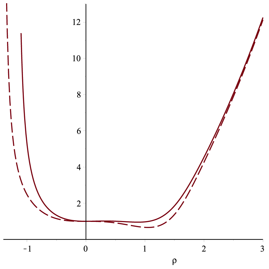
Figure 4: Behaviour of the superpotential WW for different values of the parameters: solid line corresponds to α=0=c1\alpha=0=c_{1}, β=−1\beta=-1, γ=−2\gamma=-2; dash line α=0=c1=β\alpha=0=c_{1}=\beta, γ=−2\gamma=-2.

Combining the operators AA and A†A^{\dagger} we can construct Hamiltonians

ℋ−=A†​A=−d2d​ρ2+V−​(ρ),ℋ+=A​A†=LT=−d2d​ρ2+V+​(ρ)\mathcal{H}_{-}=A^{\dagger}A=-\frac{d^{2}}{d\rho^{2}}+V_{-}(\rho),\quad\mathcal{H}_{+}=AA^{\dagger}=L_{T}=-\frac{d^{2}}{d\rho^{2}}+V_{+}(\rho)

where V+V_{+} and V−V_{-} are the supersymmetric partner potentials and they are given by

V±​(ρ)=W2​(ρ)±d​Wd​ρ.V_{\pm}(\rho)=W^{2}(\rho)\pm\frac{dW}{d\rho}.

Clearly, V+​(ρ)=Ω​(ρ)V_{+}(\rho)=\Omega(\rho) and moreover the other partner potential can be expressed as
V−​(ρ)=2​W2​(ρ)−Ω⁡(ρ)=Ω⁡(ρ)−2​d​Wd​ρ.V_{-}(\rho)=2W^{2}(\rho)-\Omega(\rho)=\Omega(\rho)-2\frac{dW}{d\rho}.
Refer to caption
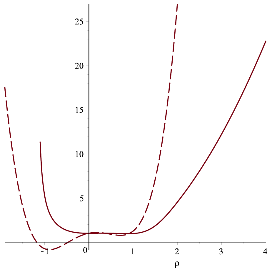
Figure 5: Behaviour of the partner potentials V−V_{-} (solid line) and V+V_{+} (dash line) for α=0\alpha=0, β=−1\beta=-1, γ=−2\gamma=-2, c1=0c_{1}=0.

If we denote the eigenstates of the Hamiltonians ℋ−\mathcal{H}_{-} and ℋ+\mathcal{H}_{+} by vn(−)v_{n}^{(-)} and vn(+)v_{n}^{(+)}, respectively, then vn(±)v_{n}^{(\pm)} must satisfy the eigenvalue equations

ℋ−​vn(−)=En(−)​vn(−),ℋ+​vn(+)=En(+)​vn(+).\mathcal{H}_{-}v_{n}^{(-)}=E^{(-)}_{n}v_{n}^{(-)},\quad\mathcal{H}_{+}v_{n}^{(+)}=E^{(+)}_{n}v_{n}^{(+)}.

In order to establish whether or not the supersymmetry is unbroken we need to find out if the ground state of ℋ−\mathcal{H}_{-} has zero energy, that is E0(−)=0E^{(-)}_{0}=0.

VI Analysis of the zero energy state

Let ψ0\psi_{0} denote the zero energy solution, i.e. E=0E=0, associated to an Hamiltonian H0H_{0} such that H0​ψ0=0H_{0}\psi_{0}=0 and H0=d2/d​r2+Ve​f​f​(r)H_{0}=d^{2}/dr^{2}+V_{eff}(r) where the effective potential has been already computed in Section II. For the potential V3V_{3} with e0=e1=e2=0e_{0}=e_{1}=e_{2}=0 corresponding to the choice a0=a1=a2=0a_{0}=a_{1}=a_{2}=0 we find that the zero energy solution can be written as a linear combination of Bessel functions as follows

ψ0​(r)=r​[C1​J7/6​(2​e43​r3/2)+C2​Y7/6​(2​e43​r3/2)]\psi_{0}(r)=\sqrt{r}\left[C_{1}J_{\sqrt{7}/6}\left(\frac{2\sqrt{e_{4}}}{3}r^{3/2}\right)+C_{2}Y_{\sqrt{7}/6}\left(\frac{2\sqrt{e_{4}}}{3}r^{3/2}\right)\right]

with integration constants C1C_{1} and C2C_{2}. This solution is not square integrable since it oscillates asymptotically as a plane wave. Therefore, it is obvious that we are handling here the scattering solution for a spacial case of the energy. Note that from the definition of e4e_{4} we can conclude that it is always strictly positive. Another case that can be solved exactly is the following. Consider the potential V4V_{4} and let a0=a2=b0=0a_{0}=a_{2}=b_{0}=0. Then, the coefficients v1v_{1}, v3v_{3}, and v4v_{4} vanishes whereas v0=−a1/b1v_{0}=-a1/b_{1}. Hence, we have

V4​(r)=−536​r2+v5​r2+v0V_{4}(r)=-\frac{5}{36r^{2}}+v_{5}r^{2}+v_{0}

with v5>0v_{5}>0. For the above potential the Schrödinger equation

d2​ψd​r2+V4​(r)​ψ​(r)=E​ψ​(r)\frac{d^{2}\psi}{dr^{2}}+V_{4}(r)\psi(r)=E\psi(r)

can be exactly solved in terms of a linear combination of Whittaker functions given by

ψE​(r)=1r​[C1​Mα,β​(i​v5​r2)+C2​Wα,β​(i​v5​r2)]\psi_{E}(r)=\frac{1}{\sqrt{r}}\left[C_{1}M_{\alpha,\beta}(i\sqrt{v_{5}}r^{2})+C_{2}W_{\alpha,\beta}(i\sqrt{v_{5}}r^{2})\right]

with

α=i⁡(E−v0)4​5,β=1412.\alpha=\frac{i(E-v_{0})}{4\sqrt{5}},\quad\beta=\frac{\sqrt{14}}{12}.

Observe that if E=v0E=v_{0} or E=0E=0 and v0=0v_{0}=0 we find that

ψE=v0​(r)=r​[C1​Jβ​(v52​r2)+C2​Yβ​(v52​r2)].\psi_{E=v_{0}}(r)=\sqrt{r}\left[C_{1}J_{\beta}\left(\frac{\sqrt{v_{5}}}{2}r^{2}\right)+C_{2}Y_{\beta}\left(\frac{\sqrt{v_{5}}}{2}r^{2}\right)\right].

References

  • [1] S. Flügge, Practical Quantum Mechanics, Springer-Verlag: Berlin, Heidelberg, New York, 1999
  • [2] J. Dereziński and M. Wrochna, “Exactly Solvable Schrödinger Operators”, Ann. Henri Poincaré 12 (2011) 397 and references therein
  • [3] A. Lamieux and A. K. Bose, ”Construction de potentiels pour lesquels l’equation de Schrödinger est soluble”, Annales de l’Inst. H. Poincaré X (1969) 259
  • [4] G. A. Natanzon, “Study of the one-dimensional Schrödinger equation generated from the hypergeometric equation”, Vestn. Leningr. Univ. 10 (1971) 22
  • [5] G. Natanson, “Heun-Polynomial Representation of Regular-at-Infinity Solutions for the Basic SUSY Ladder of Hyperbolic Pöschl-Teller Potentials Starting from the Reflectionless Symmetric Potential Well”, arXiv:1410.1515 (2014)
  • [6] D. Batic, R. Williams and M. Nowakowski, “Potentials of the Heun class”, J. Phys. A: Math. Theor. 46 (2013) 245204
  • [7] R. Milson, “Liouville Transformation and Exactly Solvable Schrodinger Equations”, Int. J. Theor. Phys. 37 (1998) 1735
  • [8] A. Messiah, Quantum Mechanics, North Holland Publishing Company, 1967
  • [9] S. C. Zhang, T. H. Hansen and S. Kivelson, “Effective-Field-Theory Model for the Fractional Quantum Hall Effect”, Phys. Rev. Lett. 62 (1989) 82
  • [10] A. Fetter, C. Hanna and R. Laughlin, “Random-phase approximation in the fractional-statistics gas”, Phys. Rev. B 39 (1989) 9679
  • [11] P. B. Wiegmann, “Superconductivity in strongly correlated electronic systems and confinement versus deconfinement phenomenon”, Phys. Rev. Lett. 60 (1988) 821
  • [12] A. M. Polyakov”, “Fermi-Bose transmutations induced by gauge fields”, Mod. Phys. Lett. A 3 (1988) 325
  • [13] A. Lerda, Anyons: Quantum Mechanics of Particles with Fractional Statistics, Springer Verlag, 1992
  • [14] C. Manuel and R. Tarrach, “Contact Interactions of Anyons”, Phys. Lett. B 268 (1991) 222
  • [15] B. Roy, A. O. Barut and P. Roy, “On the dynamical group of the system of two anyons with Coulomb interaction”, Phys. Lett. A 172 (1993) 316
  • [16] A. Ronveaux, Heun’s Differential Equations, Oxford University Press, 1995
  • [17] F. Hioe, D. MacMillen and E. Montroll, “Quantum theory of anharmonic oscillators. II. Energy levels of oscillators with x2​αx^{2\alpha} anharmonicity”, J. Math. Phys. 17 (1976) 1320
  • [18] J. Q. Liang and H. J. W. Müller-Kirsten, “Anharmonic Oscillator Equations: Treatment Parallel to Mathieu Equation”, Transactions of the IRE Professional Group (2004), arXiv:quant-ph/0407235
  • [19] A. Schulze-Halberg, “Quasi-Exactly Solvable Singular Fractional Power Potentials Emerging from the Triconfluent Heun Equation”, Phys. Scr. 65 (2002) 373
  • [20] K. Bay, W. Lay and A. Akopyan, “Avoided Crossings of the quartic oscillator”, J. Phys. A: Math. Gen. 30 (1997) 3057
  • [21] A. Ushveridze, Quasi-exactly solvable models in quantum mechanics, Inst. of Physics Publ., Bristol, 1994
  • [22] A. K. Bose, “A Class of Solvable Potentials”, Nuovo Cim. 32 (1964) 679
  • [23] I. S. Gradshteyn and I. M. Ryzbik, Table of Integrals, Series, and Products, Academic Press, 2007
  • [24] L. Yang, “Recent Advances on Determining the Number of Real Roots of Parametric Polynomials”, J. Symb. Comp. 28 (1998) 225
  • [25] A. Eremenko, A. Gabrielov and B. Shapiro, High-energy eigenfunctions of one-dimensional Schrödinger operators with polynomial potentials, Comp. Meth. Function Theory 8 (2008) 513
  • [26] F. A. Berezin and M. A. Shubin, The Schrödinger equation, Kluwer, Dordrecht, 1991
  • [27] Y. Sibuya, Global theory of a second order linear ordinary differential equation with a polynomial coefficient, North-Holland Publishing Co., Amsterdam-Oxford,1975
  • [28] A. Eremenko, A. Gabrielov and B. Shapiro, Zeroes of eigenfunctions of some anharmonic oscillators, Ann. Inst. Fourier, Grenoble,58 (2008) 603
  • [29] S. Elaydi, An Introduction to Difference Equations, Springer Verlag, 2000
  • [30] A. Decarreau, P. Maroni and A. Robert, “Sur les equations confluentes de l’equation de Heun”, Ann. Soc. Sci. Brux. 92 (1978) 151
  • [31] G. D. Birkhoff, “ Formal theory of irregular linear difference equations”, Acta Math. 54 (1930) 205
  • [32] G. D. Birkhoff and W. J. Trjitzinsky, “Analytic theory of singular difference equations”, Acta Math. 60 (1932) 1
  • [33] J. Wimp, Computation with Recurrence Relations, Pitman Press, 1984