Cosmological Constraints From Weak Lensing Peak Statistics With CFHT Stripe 82 Survey

In the weak lensing theory under the framework of general relativity, the deflection of light rays from a source can be written as the gradient of a lensing potential $\psi(\boldsymbol{\theta})$. The induced observational effects can be described by the Jacobian matrix $\boldsymbol{A}$, which is given by (Bartelmann & Schneider, 2001, e.g.,)

where the convergence $\kappa$ and the shear $\gamma_{i}$ lead to the isotropic change and the elliptical shape distortion of the observed image, respectively, with respect to the unlensed image. They are related to the potential by

In the weak lensing regime under the Born approximation, we have

where $H_{0}$ is the Hubble constant, $\chi$ is the comoving radial distance, $f_{K}$ is the comoving angular diameter distance, $a$ is the scale factor of the universe, and $\delta$ is the density perturbation along the line of sight.

The convergence $\kappa$ is directly related to the projection of line-of-sight density fluctuations weighted by the lensing efficiency factor. Physically, massive structures generate large weak lensing signals along their lines of sight. These peak signals are best seen visually in the weak lensing convergence field. On the other hand, weak lensing signals directly extracted from galaxy shape measurements are the shears, or more precisely the reduced shears defined as $g_{i}=\gamma_{i}/(1-\kappa)$, rather than the convergence. Therefore weak lensing peak analysis usually involves procedures to construct quantities representing the projected mass distribution from lensing shears based on the relation between the two quantities shown in Eqn.(3).

Specifically, assuming precise shape measurements, the observed ellipticity of a galaxy at redshift $z$ located at the sky position $\boldsymbol{\theta}$ can be written in a complex form given by (Seitz & Schneider, 1997, e.g.,)

where ‘*’ represents the complex conjugate operation, $\boldsymbol{g}=g_{1}+ig_{2}$ is the complex reduced shear, and $\boldsymbol{\epsilon}_{s}$ is the intrinsic ellipticity of the galaxy. Here the complex ellipticity is defined as $\boldsymbol{\epsilon}=(a-b)/(a+b)\exp(2i\phi)$ with $a$, $b$ and $\phi$ being the length of the major and minor axes and the orientation of the approximate ellipse of the observed image, respectively. For source galaxies at a fixed redshift $z$, it has been shown that the average of $\boldsymbol{\epsilon}$ over a large number of galaxies near $\boldsymbol{\theta}$ gives rise to an unbiased estimate of $\boldsymbol{g}(\boldsymbol{\theta},z)$ or $1/{\boldsymbol{g}}(\boldsymbol{\theta},z)$ assuming $\langle\boldsymbol{\epsilon}_{s}\rangle=0$. For galaxies with a redshift distribution, the average of $\boldsymbol{\epsilon}$ over galaxies near a given sky position may have a complicated relation with the lensing signal we are interested in if both $|\boldsymbol{g}|<1$ and $|\boldsymbol{g}|>1$ occur in the region for galaxies at different redshifts. On the other hand, for sub-critical regions with $|\boldsymbol{g}|<1$ for all the redshifts, the average of the observed ellipticity $\langle\boldsymbol{\epsilon}\rangle$ gives rise to an estimate of $\langle\boldsymbol{g}\rangle$ weighted by the redshift distribution of source galaxies. In the case $\kappa\ll 1$, we have $\langle\boldsymbol{\epsilon}\rangle\approx\langle\boldsymbol{\gamma}\rangle$. For the weak lensing peak analysis, we therefore need to construct a field closely related to the matter distribution from the (reduced) shear estimate $\langle\boldsymbol{\epsilon}\rangle$.

The aperture mass peak analysis, also referred to as the shear peak analysis, is to study peaks in the aperture mass $\rm M_{\rm ap}$ field constructed from the tangential shear component with respect to the point of interest with a filtering function $Q$ (Schneider et al., 1998; Marian et al., 2012; Bard et al., 2013, e.g.,). Theoretically, $\rm M_{\rm ap}$ corresponds to the convergence field filtered with a compensated window function $U$ where $U$ and $Q$ are related. One of the advantages of $\rm M_{\rm ap}$ studies is that because of the compensated nature of $U$, $\rm M_{\rm ap}$ is independent of the lensing mass-sheet degeneracy. Furthermore, in the case with $\kappa\ll 1$ and $\boldsymbol{g}\approx\boldsymbol{\gamma}$, $\rm M_{\rm ap}$ can be obtained directly from the tangential component of the observed $\langle\epsilon_{t}\rangle$. In the peak regions where the lensing signals are high, the difference between $\boldsymbol{g}$ and $\boldsymbol{\gamma}$ is not negligible. Therefore noting that the $\rm M_{\rm ap}$ constructed from $\langle\epsilon_{t}\rangle$ itself carries cosmological information, it is not the same as the filtered convergence field.

Another approach for weak lensing peak studies is to reconstruct the convergence field from $\langle\boldsymbol{\epsilon}\rangle$ taking into account the nonlinear relation between $\boldsymbol{g}$ and $\boldsymbol{\gamma}$ (Kaiser & Squires, 1993; Kaiser et al., 1995; Seitz & Schneider, 1995; Bartelmann, 1995; Squire & Kaiser, 1996; Seitz & Schneider, 1997; Jauzac et al., 2012; Jullo et al., 2014, e.g.,). In this approach, to avoid unphysical results, it is important to filter $\boldsymbol{\epsilon}$ first and then to proceed with convergence reconstruction using the filtered $\langle\boldsymbol{\epsilon}\rangle$. Different reconstruction schemes have been studied. For the classical Kaiser-Squires (KS) reconstruction (Kaiser & Squires, 1993; Squire & Kaiser, 1996), boundary effects and the mass-sheet degeneracy problem can exist. However, for a field of view of about $1\deg\times 1\deg$ and larger, such effects are expected to be insignificant. In this paper, we reconstruct the convergence field from the filtered $\langle\boldsymbol{\epsilon}\rangle$ with the nonlinear KS method (Bartelmann, 1995, e.g.,). From numerical simulations, we find that the regions with $|\boldsymbol{g}|>1$ are negligible, and therefore assuming sub-criticality for all the regions is an excellent approximation.

Our convergence reconstruction procedures are described below.

For a source galaxy used in weak lensing analyses in the CS82 catalogue, we first correct the additive errors

where $\epsilon_{i}$ and $\epsilon_{i}^{c}$ are the uncorrected and corrected ellipticity components, respectively, and $c_{2}$ is the additive bias given by CS82. With $\epsilon_{i}^{c}$, we apply smoothing and obtain a smoothed field of $\boldsymbol{\epsilon}$ on regular $1024\times 1024$ grids over the field of view of one pointing. With the multiplicative errors $m$ taken into account statistically (van Waerbeke et al., 2013), we have

where $\boldsymbol{\theta}$ and $\boldsymbol{\theta}_{j}$ are for the grid position and the galaxy position, respectively, $W_{\theta_{\rm G}}$ is the normalised smoothing function, $w$ is the weight for source galaxy shape measurements given by CS82. The summation is over all the source galaxies. In the subcritical approximation, $\langle{\boldsymbol{\epsilon}}\rangle(\boldsymbol{\theta})$ is an unbiased estimate of $\langle\boldsymbol{g}\rangle$ smoothed over the window function $W_{\theta_{\rm G}}$ and weighted by the source redshift distribution. We use the Gaussian smoothing function $W_{\theta_{\rm G}}$ with

The smoothing scale $\theta_{\rm G}$ is chosen to be $\theta_{\rm G}=1.5$ arcmin, suitable for cluster-scale structures that are closely related to high weak lensing peaks. Within the smoothing kernel, the number of galaxies is about $n_{g}\theta_{\rm G}^{2}\sim 20$, for $n_{g}\sim 10\hbox{ arcmin}^{-2}$. We expect that the statistics of the residual shape noise after smoothing is approximately Gaussian from the central limit theorem (van Waerbeke, 2000, e.g.).

With $\langle{\boldsymbol{\epsilon}}\rangle(\boldsymbol{\theta})$, we perform the convergence reconstruction iteratively by using the relation between $\kappa$ and $\gamma$ in Eqn. (3). Particularly, we use their relation in Fourier space with

and

We start by assuming $\kappa^{(0)}=0$ everywhere, and thus $\boldsymbol{\gamma}^{(0)}=\langle\boldsymbol{\epsilon}\rangle$ (Bartelmann, 1995). At ${n}$-th step, we obtain $\kappa^{(n)}$ from $\boldsymbol{\gamma}^{(n-1)}$ via Eqn.(9) and the subsequent inverse Fourier transformation. We then update $\boldsymbol{\gamma}$ to $\boldsymbol{\gamma}^{(n)}=(1-\kappa^{(n)})\langle\boldsymbol{\epsilon}\rangle$ for next iteration. The reconstruction process is stopped when the converging accuracy of $10^{-6}$ (the maximum difference of the reconstructed convergence between the two sequential iterations) is reached. For CS82, the reconstruction is done pointing by pointing each with the field of view of about $1\deg\times 1\deg$.

To evaluate the shape noise level in each pointing for subsequent peak analyses, we randomly rotate the corrected ellipticity of each galaxy. Then the same procedure is applied to obtain the reconstructed random noise convergence field.

It is noted that there are regions with no reliable shape measurements for galaxies indicated with the index MASK$>$1 in the CS82 catalogue. These galaxies are excluded in the weak lensing analyses. The existence of these masked regions can affect the weak lensing peak abundances significantly if they are not treated properly. In LWPF2014, we study in detail the mask effects. With the signal-to-noise ratio defined by the average noise level, the number of high peaks increases around the masked regions, which can lead to considerable bias in cosmological parameter constraints derived from weak lensing peak abundances. To reduce the mask effects, regions around masks should be excluded in peak counting. If they are kept, the noise effects in these regions should be considered separately from the regions away from masks (LWPF2014).

To quantify the mask effects on the number of usable galaxies in the convergence reconstruction, we calculate the galaxy filling factor at each grid point similar to that done in van Waerbeke et al. (2013). Summing over galaxies outside masked regions, we define the galaxy filling factor as

where $f_{0}$ is calculated by randomly populating galaxies over the full area of a tile with

Here $\langle\rangle$ is for the average over $\boldsymbol{\theta}$. Specifically, for each tile, we calculate the average number density of galaxies in the area excluding the masked regions. With this number density, we then randomly populate galaxies over the full area of the tile including the masked regions. For each galaxy, we randomly assign it a weight $\tilde{w}$ according to the weight distribution of the real observed galaxies. We then calculate the quantity $\sum_{n}W_{\theta_{\rm G}}(\boldsymbol{\theta_{n}}-\boldsymbol{\theta})\tilde{w}(\boldsymbol{\theta_{n}})$ at each grid point $\boldsymbol{\theta}$ where the summation is over all the populated galaxies. The average value over all the grid points gives rise to $f_{0}$.

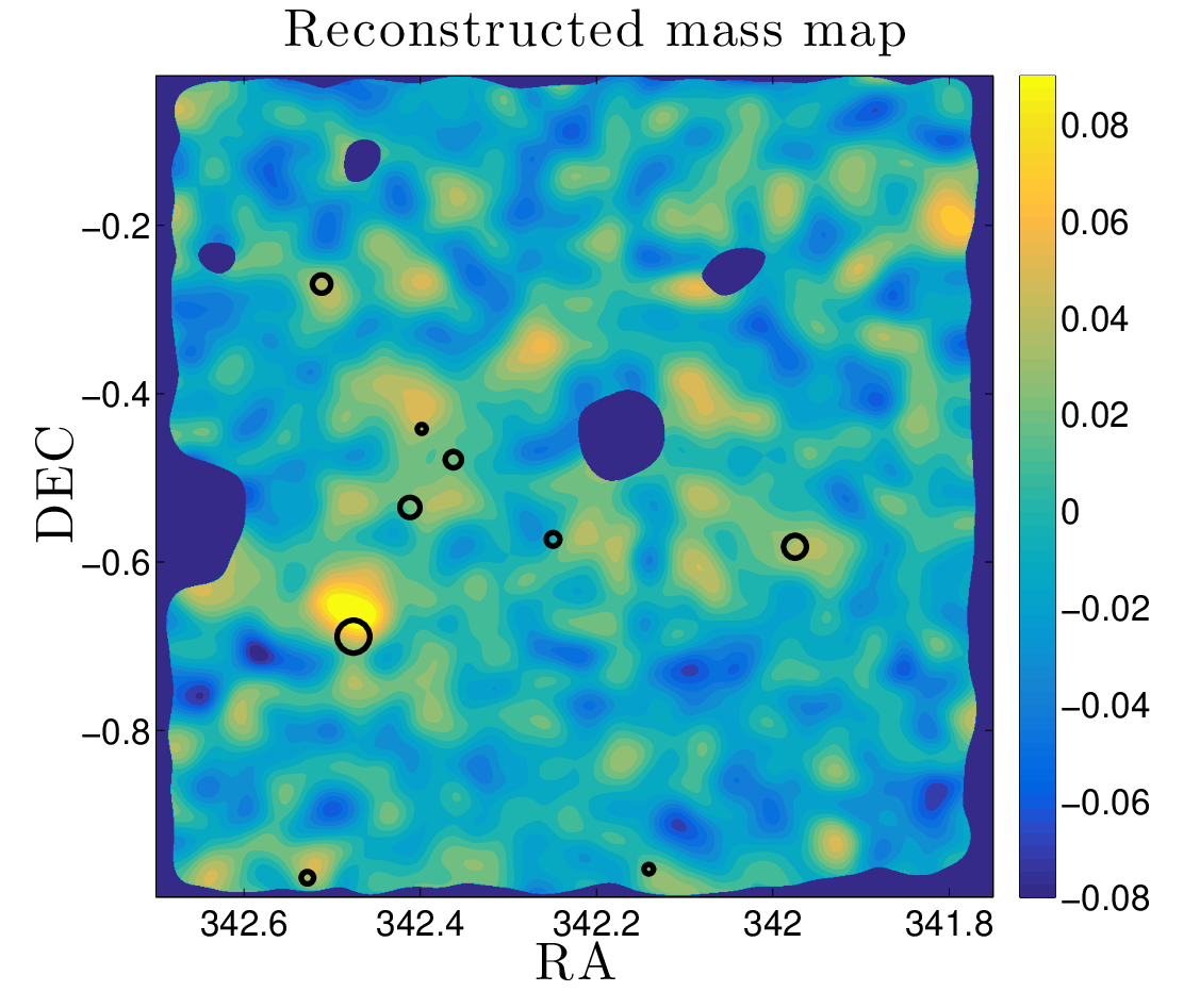
Hence, for each pointing, we obtain the reconstructed lensing convergence, noise and filling factor maps, respectively. We have a total of $173$ sets of maps corresponding to the $173$ pointings. In Figure 2, we show an example of the reconstructed convergence map for one pointing and the corresponding map of the filling factor. In each map, the dark blue regions are regions with the filling factor $f<0.5$. To avoid the mask effects on weak lensing peak analyses, we exclude these regions in peak counting (van Waerbeke et al., 2013, LWPF2014;). The black circles in the plots show the clusters in the field detected using the red-sequence Matched-filter Probabilistic Percolation (redMaPPer) algorithm (Rykoff et al., 2014). It is seen that the clusters have a good association with weak lensing convergence peaks, but the correspondence is not one to one due to the existence of noise and the projection effects of large-scale structures (Shan et al., 2014, e.g.,).

For weak lensing peak analyses, we detect peaks from the reconstructed lensing convergence maps as follows. Considering a pixel on a reconstructed convergence map ($1024\times 1024$ pixels), if its convergence value is the highest among its nearest 8 neighbouring pixels, it is identified as a peak. We only count peaks in regions with the filling factor $f>0.5$. To reduce the boundary effects, we also exclude the outer most 50 pixels (corresponding to $\sim 3\hbox{ arcmin}\sim 2\theta_{\rm G}$) in each of the four sides of a map in our peak counting. The effective area of CS82 for weak lensing peak studies is then reduced to $\sim 114\deg^{2}$ after mask-region and boundary exclusions. The signal-to-noise ratio of a peak is defined by

where $K$ is the reconstructed convergence value of the peak and $\sigma_{0}$ is the mean rms of the noise from the $173$ noise maps. It is known that $\sigma_{0}$ depends on the number density of source galaxies and the smoothing scale of the window function used in obtaining the smoothed ellipticity field $\langle\epsilon\rangle$. It can vary somewhat from one pointing to another. In our study, the mean $\sigma_{0}$ is evaluated from all the noise maps considering only regions with the filling factor $f>0.5$. For the smoothing scale $\theta_{\rm G}=1.5$ arcmin, we have $\sigma_{0}\approx 0.022$. It is noted that we calculate $\sigma_{0}$ directly from the rotated galaxies in noise maps, and therefore we do not need to know explicitly the galaxy intrinsic ellipticity dispersion $\sigma_{\epsilon}$. On the other hand, we find that for CS82 galaxies, $\sigma_{\epsilon}\sim 0.4$ for the total of the two components.

We note that in our peak identification scheme, we do not group peaks together as some other methods do (Hamana et al., 2012, e.g.,). We will see in §3.3 that our theoretical model for peak abundances takes into account the noise peaks in halo regions and counts them as independent ones. Accordingly, we therefore do not need the peak grouping that may give rise to some artificial effects.

To derive cosmological constraints from observed weak lensing peak abundances, their dependence on cosmological models needs to be understood and quantified. Known to be closely related to line-of-sight matter concentrations, the existence of galaxy shape noise, the projection effects of large-scale structures, the complex mass distribution of dark matter halos, etc., complicates the relation between weak lensing peak abundances and the underlying mass function of dark matter halos. While building a large set of templates from numerical simulations densely sampled over the multi-dimensional cosmological parameter space can be very useful and important, it is computationally expensive. On the other hand, theoretical modelling based on our physical understandings can be very insightful and valuable in disentangling different effects on weak lensing peak abundances. With explicit dependences on cosmological parameters and other physical parameters, it can be used to perform cosmological constraints efficiently. Depending on the assumptions and approximations employed in the modelling, their results can be less accurate than those from full simulations. Similarly to the calculation of the nonlinear matter power spectrum based on the halo model but calibrated with simulations, which is widely used in weak lensing two-point correlation analyses, the combination of the two, that is, testing and calibrating a model with simulations, can be a very effective way to study the cosmological dependence of weak lensing peak statistics efficiently with high precision.

In this paper, we focus mainly on high peaks and adopt the model of F10 for the weak lensing peak abundances, which takes into account the dominant shape noise in the modelling. The model has been tested extensively by comparing with full ray-tracing simulations (F10, LWPF2014), and has also be confronted with observational studies (Shan et al., 2012; Shan et al., 2014).

Here we describe the important ingredients of the model. More details can be found in F10 and LWPF2014.

In F10, we assume that the smoothed convergence field can be written as $K_{N}=K+N$, where $K$ represents the true lensing convergence, and $N$ is for the residual shape noise. The field $N$ results from the contribution of the intrinsic ellipticities of different galaxies in the smoothing kernel. Without considering the intrinsic alignments of source galaxies, if the number of galaxies within the smoothing kernel is large enough, it has been shown that $N$ is approximately a Gaussian random field from the central limit theorem (e.g., van Waerbeke 2000). As discussed in §3.2, for a smoothing scale $\theta_{\rm G}=1.5\hbox{ arcmin}$, the number of galaxies within the smoothing window in CS82 is $\sim 20$. Therefore $N$ can be well approximated as a Gaussian random field.

Concentrating on high peaks, it is expected that signals of true peaks mainly come from individual massive halos (Hamana et al., 2004; Tang & Fan, 2005; Yang et al., 2011, e.g.,). We therefore divide a given area into halo regions and field regions. Inside the region of an individual halo, we have $K_{N}=K+N$, where $K$ is regarded as a known field from the halo convergence, and $N$ is a Gaussian random field. Therefore $K_{N}$ itself is also a Gaussian random field modulated by the halo surface mass distribution $K$. Then the peak number distribution for $K_{N}$ is readily calculable using Gaussian statistics. The modulation effects from $K$ involve $K$ itself, its first derivatives $K^{i}=\partial K/\partial x_{i},(i=1,2)$ and its second derivatives $K^{ij}=\partial^{2}K/\partial x_{i}\partial x_{j}$. The total number of peaks in halo regions can thus be obtained by the summation of the peaks over all the halo regions weighted by the halo mass function. In the field region, the numbers of peaks are directly computed from the noise field $N$.

Specifically, the total surface number density of peaks can then be written as

where $\nu=K_{N}/\sigma_{0}$ is the signal-to-noise ratio of a peak. The term $n_{\mathrm{peak}}^{c}(\nu)$ is for peaks in halo regions including not only the true peaks corresponding to real halos but also the noise peaks within the halo regions. The second term $n_{\mathrm{peak}}^{n}(\nu)$ is for pure noise peaks in field regions.

For $n_{\rm peak}^{c}(\nu)$ in halo regions, it can be written as

where $dV(z)$ is the cosmological volume element at redshift z, $d\Omega$ is the solid angle element, $n(M,z)$ is the mass function of dark matter halos. Here we adopt the Sheth-Tormen mass function in the calculation (Sheth & Tormen, 1999). The mass limit $\rm M_{\rm lim}$ is for the mass above which individual halos contribute dominantly to the weak lensing peak signals along their lines of sight. From simulation analyses, we find that $\rm M_{\rm lim}=10^{13.7}h^{-1}\hbox{M}_{\odot}$ is a suitable choice. The factor $f_{p}$ is for the number of peaks in the area within the virial radius of a halo of mass $M$ at redshift $z$, and is given by

where $\theta_{\rm vir}=R_{\rm vir}(M,z)/D_{A}(z)$, and $D_{A}(z)$ is the angular-diameter distance. The physical virial radius is calculated by

where $\rho(z)$ is the background matter density of the Universe at redshift $z$ and the overdensity $\Delta_{\rm vir}$ is taken from Henry (2000).

The function $\hat{n}^{c}_{\mathrm{peak}}(\nu,\theta,M,z)$ in Eqn.(16) describes the surface number density of peaks at the location of $\theta$ from the centre of the halo, which depends on the convergence profile of the halo. On the basis of the theory of Gaussian random fields, it can be derived explicitly as (F10)

where $\theta_{*}^{2}=2\sigma_{1}^{2}/\sigma_{2}^{2}$, $\gamma_{N}=\sigma_{1}^{2}/(\sigma_{0}\sigma_{2})$, $K^{i}=\partial_{i}K$, and $K^{ij}=\partial_{ij}K$. Here the quantities $\sigma_{i}$ are the moments of the noise field $N$ given by (e.g. van Waerbeke 2000)

where $N(k)$ is the Fourier transform of the noise field $N$. For $K(\theta)$, $K^{i}(\theta)$, and $K^{ij}(\theta)$ of a halo with mass $M$ at redshift $z$, they depend on the mass profile of the halo and source redshift distribution. Here we assume the spherical Navarro-Frenk-White (NFW) mass distribution for dark matter halos (Navarro et al., 1996; Navarro et al., 1997). The concentration parameter $c_{\rm vir}(M)=R_{\rm vir}/r_{\rm s}$ is calculated from the mass-concentration relation given in Bhattacharya et al. (2013) where $r_{s}$ is the characteristic scale of an NFW halo. For the redshift distribution of source galaxies, we take Eqn. (1) for CS82 data.

The function $F(x_{N})$ in Eqn. (18) is given by (F10)

where $x_{N}=(\lambda_{N1}+\lambda_{N2})/\sigma_{2}$ and $e_{N}=(\lambda_{N1}-\lambda_{N2})/(2\sigma_{2}x_{N})$. $\lambda_{N1}$ and $\lambda_{N2}$ are the two eigenvalues $(\lambda_{N1}\geq\lambda_{N2})$ and $\theta_{N}$ is the rotation angle in the range $[0,\pi]$ with the diagonalisation of $(-K_{N}^{ij})$ (Bardeen et al., 1986; Bond & Efstathiou, 1987, e.g.,).

As for the field term $n_{\mathrm{peak}}^{n}(\nu)$ in Eqn. (14), it is given by

where $n_{\mathrm{ran}}(\nu)$ is the surface number density of pure noise peaks without foreground halos. It can be calculated by Eqn. (18) with $K=0$, $K^{i}=0$ and $K^{ij}=0$.

It is seen that in this model, the cosmological information is contained in the halo mass function, lensing kernel, cosmic volume element, and the density profile of dark matter halos. We note that although we use the NFW density profile and the mean mass-concentration relation derived by Bhattacharya et al. (2013) for the full sample of dark matter halos in our fiducial model calculations, in principle, the density profile parameters can be treated as free parameters. Therefore from weak lensing peak abundances, it is possible to constrain these structural parameters simultaneously with cosmological parameters.

For our model calculation of $n_{\rm peak}$, multi-dimensional integrations are needed. With great efforts numerically and applying multiple parallel techniques, such as OpenMP and GPU programming, we have developed a fast and high precision model calculation algorithm, which makes it possible for us to perform cosmological constraints from weak lensing peak abundances. An outline of our programming structures is given in the Appendix.

As described in §3.2, from the reconstructed convergence maps, we identify and count peaks in regions where the galaxy filling factor is $f>0.5$. This effectively excludes the masked regions in the peak counting to avoid the mask effects. The useful survey area is approximately $114\deg^{2}$. We only consider high peaks with the signal-to-noise ratio $\nu\geq 3$. With the noise level $\sigma_{0}\sim 0.022$ under the smoothing scale $\theta_{G}=1.5\hbox{ arcmin}$ for CS82, the high peaks have smoothed signals $K\geq 0.066$. For the considered survey area, there are few peaks with $\nu>6$. We therefore concentrate on the peaks in the range of $3\leq\nu\leq 6$.

We divide the peaks into $5$ bins. We consider both equal bins with $\Delta\nu=0.5$ and unequal bins with the number of peaks comparable in different bins. For equal bins, we do not include the number of peaks in the bin of $\nu=(5.5,6]$ in cosmological studies because it is only $\sim 1$ with large expected statistical fluctuations. In this case, the number of peaks is $\sim 500$ for the first bin with $\nu=[3,3.5]$ and is $\sim 10$ for the last bin with $\nu=(5,5.5]$. For unequal bins, we have the number of peaks in the range of $(\sim 160,\sim 80)$ for different bins with $\nu=[3,3.1],(3.1,3.25],(3.25,3.5],(3.5,4],(4,6]$, respectively.

To derive cosmological parameter constraints from weak lensing peak counts, we calculate the $\chi^{2}$ defined as follows (LWPF2014)

where $dN_{i}^{(p^{\prime})}=N_{\rm peak}^{(p^{\prime})}(\nu_{i})-N_{\rm peak}^{(d)}(\nu_{i})$ with $N_{\rm peak}^{(p^{\prime})}(\nu_{i})$ being the prediction for the cosmological model $p^{\prime}$ from F10 and $N_{\rm peak}^{(d)}(\nu_{i})$ being the observed data for the peak counts. This effectively assumes that the number fluctuation in each bin can be approximated by a Gaussian distribution. With the number of peaks in the equal bin case being larger than $\sim 10$ per bin and being larger than about $80$ per bin in the unequal bin case, the Gaussian error distribution is expected to be a good approximation. The corresponding likelihood function is given by

The matrix $C_{ij}$ is the covariance matrix of the peak counts including the error correlations between different $\nu$ bins. Here we apply bootstrap analyses using the CS82 observational data themselves to obtain an estimate of $C_{ij}$. We realise that such an estimate cannot reveal the cosmic variance over the full survey area. Ideally, $C_{ij}$ should be constructed by generating a large number of CS82 mocks from ray-tracing simulations following exactly the same galaxy distribution, mask distribution, survey geometry, etc. as CS82 data. It is noted that the CS82 survey covers a long stripe of $\sim 90\deg\times 2\deg$. Therefore to fully mimic the survey geometry, we need very large simulations to cover the $\sim 90\deg$ extension, which are difficult to achieve at the moment.

For $C_{ij}$, we thus generate $10000$ bootstrap samples by resampling the 173 tiles from real observation data sets. The covariance matrix $C_{ij}$ is then calculated from the bootstrap samples by

where $r$ denotes for different samples with the total number of samples $R=10000$, and $N^{r}_{\rm peak}(\nu_{i})$ is for the peak count in the bin centred on $\nu_{i}$ from the sample $r$. The inverse of the covariance matrix is then calculated by Hartlap et al. (2007)

where $N_{\mathrm{bin}}$ is the number of bins used for peak counting.

We note that such bootstrap analyses implicitly assume the independence of the peak distribution between different tiles each with an area of about $1\deg^{2}$. We have made a test by dividing the survey area into units each containing $4$ adjacent tiles (i.e., $\sim 2\deg\times 2\deg$) and then performing bootstrap analyses by resampling these units. The resulted inverse covariance, considering the diagonal elements which are much larger than the off-diagonal terms, shows less than $\sim 8\%$ differences from the one using one tile as a unit. We also perform tests using $2\times 3$ and $2\times 10$ adjacent tiles as units, separately. The diagonal terms of the inverse covariance differ from those using one tile as a unit by $\leq 8\%$ and $\leq 11\%$, respectively. We have carried out another test to use our 15 sets of mocked data to calculate the covariance. However, our mock simulations do not mimic the long stripe geometry of the CS82 survey, and the independent unit has an area of $4\times 3.5\times 3.5=49\deg^{2}$, as will be described in §4.2. We find that for the diagonal elements of the inverse covariance, the differences between the results from mock sets and that of using one tile as a unit are generally less than $10\%$.

We also carry out Jackknife resampling for error estimations. For using one tile, $2\times 2$ and $2\times 3$ tiles as independent units, respectively, the diagonal elements of the resulted inverse covariance differ from the corresponding bootstrap resampling by less than $5\%$.

We therefore adopt the bootstrap covariance estimated from CS82 data using one tile as an independent unit in our following fiducial analyses.

We use CosmoMC (Lewis & Bridle, 2002) modified to include our likelihood function for weak lensing peak counts to perform cosmological constraints. In this paper, we mainly consider constraints on the two cosmological parameters $(\Omega_{\rm m},\sigma_{8})$ under the flat $\Lambda$CDM assumption. We adopt flat priors in the range of $[0.05,0.95]$ and $[0.2,1.6]$ for $\Omega_{\rm m}$ and $\sigma_{8}$, respectively. We take the Hubble constant $h=0.7$ in units of $100\hbox{ }\rm{km}/\rm{s}/\rm{Mpc}$, the power index of the initial density perturbation spectrum $n_{s}=0.96$, and the present baryonic matter density $\Omega_{\rm b}=0.046$. As discussed above, our fiducial constraints use the covariance estimated from bootstrap resampling of individual tiles. As a quantitative comparison, we also perform $(\Omega_{\rm m},\sigma_{8})$ constraints by using the covariance estimated from resampling $2\times 2$ adjacent tiles. The constraint contours are nearly overlapped with those of our fiducial analyses with the area of $1\sigma$ region larger only by $\sim 1\%$.

To further show the potential of weak lensing peak statistics, we also perform constraints on the mass-concentration relation of dark matter halos, assuming it follows a power law relation, simultaneously with the cosmological parameters $(\Omega_{\rm m},\sigma_{8})$.

Before presenting the results from CS82 observational data, in this part, we first show our mock CS82 analyses using ray-tracing simulations. As discussed above, the full mock of CS82 taking into account the long stripe geometry demands very large simulations, which are yet to be realised. Therefore in the current mock analyses presented here, we do not attempt to mimic the survey geometry of CS82, but are limited to the tests of our peak analyses procedures, including the convergence reconstruction, mask effects exclusion, cosmological parameter fitting, etc.. These mocks also serve as a further test of our theoretical model on the peak abundances.

To construct the CS82 mocks, we carry out dark-matter-only N-body simulations in the flat $\Lambda$CDM framework. The cosmological parameters are taken to be $\Omega_{\rm m}=0.28$, $\Omega_{\Lambda}=0.72$, $\Omega_{\rm b}=0.046$, $\sigma_{8}=0.82$, $n_{\rm s}=0.96$ and $h=0.7$. Our ray-tracing procedures largely follow our previous studies of LWPF2014, but with different box paddings.

In accord with the redshift distribution of CS82 galaxies, we perform ray-tracing calculations up to $z=3$. For our considered cosmological model, the comoving distance to $z_{s}=3$ is approximately $4.54h^{-1}\mathrm{Gpc}$. We design to pad $12$ independent simulation boxes to $z=3$, with $8$ simulation boxes each with a size of $320h^{-1}\mathrm{Mpc}$ to redshift $z=1$ and $4$ larger simulations each with a size of $600h^{-1}\mathrm{Mpc}$ from $z=1$ to $z=3$. With these independent simulations, we can perform ray-tracing calculations straightforwardly with no repeated use of same structures.

The N-body simulations are done with Gadget-2 (Springel 2005). For both small and large sized simulations, we use $640^{3}$ particles. The mass resolution is $\sim 9.7\times 10^{9}h^{-1}\rm{M}_{\odot}$ and $\sim 6.4\times 10^{10}h^{-1}\rm{M}_{\odot}$ for small boxes and large boxes, respectively. The simulations start from $z=50$ and the initial conditions are set by using 2LPTic (Crocce et al. 2006). The initial density perturbation spectrum is generated by CAMB (Lewis et al. 2000). The force softening length is about $\sim 20h^{-1}\mathrm{kpc}$, which is good enough for our studies concerning mainly high weak lensing peaks corresponding to massive dark matter halos.

For ray-tracing simulations, we use $59$ lens planes up to $z=3$. The corresponding redshifts of the planes are listed in Table 1. We follow closely the method of Hilbert et al. (2009). The detailed descriptions for ray-tracing calculations can be found in LWPF2014. In order to generate mock data for CS82 galaxies, we calculate shear and convergence maps at the far edge of each of the $59$ lensing planes using the lower redshift planes. For a set of simulations with $12$ independent boxes, we then can generate $4$ sets of lensing maps each with an area of $3.5\times 3.5\deg^{2}$ sampled on $1024\times 1024$ pixels. In each set, we have $59$ shear and $59$ convergence maps at $59$ different redshifts corresponding to the far edges of the $59$ lens planes. We run $12$ sets of simulations, and generate lensing maps with the total area of $12\times 4\times(3.5\times 3.5)=588\deg^{2}$. This allows us to generate $3$ nearly independent mocks for CS82, and each mock is constructed from $3$ sets of simulations with the area of $\sim 3\times 49=147\deg^{2}$.

For each mock, the generating procedure is as follows.

(i) With the $3\times 49\deg^{2}$ lensing maps, we place the tiles of CS82 observed galaxies behind. We note again that we do not attempt to mimic the true CS82 long stripe survey geometry here. Therefore we pad the CS82 tiles randomly over the simulated map area. In each tile, the positions and the amplitudes of ellipticities of the galaxies are preserved, but with their orientations being randomised. Because there is no exact redshift information for each galaxy, we assign redshifts to the galaxies following the redshift distribution of Eqn. (1). The galaxy weights and the mask information are also preserved in each tile.

(ii) For a galaxy, its reduced shear $\boldsymbol{g}$ is calculated by interpolating the signals from the pixel positions on simulated maps to the galaxy position. The interpolation is also done in the redshift dimension. Regarding the randomised ellipticity obtained in (i) as its intrinsic ellipticity, we then can construct the mock observed ellipticity for the galaxy by Eqn.(5).

(iii) For each tile of the mock data, we perform the convergence reconstruction with the same procedure for the observed data described in §3.2 except we do not correct for the multiplicative error in the mock data because our lensing signals are from simulations.

(iv) We perform the peak identifications and peak number counting in the same way as for the observational data described also in §3.2.

In our analyses, noise peaks from shape noise are accounted for. Therefore to obtain a good estimate of the average numbers of peaks, we randomly rotate the galaxies $5$ times leading to $5$ realizations of the intrinsic ellipticities for source galaxies. Therefore, we totally generate $3\times 5$ mocks for CS82.

In Figure 3, we show the peak number distributions for the mock data. The upper left panel is for the results (in logarithmic scale) of equal bins with the bin width $\Delta\nu=0.5$ in the range of $[3.,5.5]$ and the upper right panel (in linear scale) is for the case of unequal bins with $\nu=[3,3.1],(3.1,3.25],(3.25,3.5],(3.5,4],(4,6]$, respectively. The three sets of symbols with different colours correspond to the mocks from $3$ independent sets of simulated maps. The $5$ data points within each colour are the results from different shape noise realizations. The blue ’*’ and error bars are for the average values and rms over the $15$ mocks. The solid line is for our model predictions with the shape noise level $\sigma_{0}$ taken to be the average value over all the tiles. The lower panels show the corresponding relative differences between the average values of the $15$ mocks and our model predictions. It is seen that for both binning cases, the averaged mock results agree with our model predictions very well. The relative differences are $\leq 10\%$, and most often $\leq 5\%$.

In Figure 4 we show the derived constraints on $(\Omega_{\rm m},\sigma_{8})$. Here we use the results averaged over the $15$ mocks as the ‘observed’ data, and the covariance matrix is estimated by constructing bootstrap samples each containing $173$ tiles as the CS82 data from all the tiles in the $15$ mocks. The contours are for $1\sigma$ and $2\sigma$ confidence levels. The left and right panels are for the cases of equal bins and unequal bins, respectively. The blue symbol indicates the underlying parameters of the mocks. We see that noting the strong degeneracy of the two parameters, the mock constraints recover the input cosmological parameters excellently. The results from the two binning cases agree well.

We now proceed to show the results from the CS82 observational data. In Figure 5, the left and right panels show the results of peak counts for the equal and unequal bins, respectively. The error bars are from the bootstrap sampling using the CS82 observational tiles. The solid line in each panel is from our theoretical model with the best fit cosmological parameters (see Figure 6). In Figure 6, we show the cosmological constraints from the CS82 observed weak lensing peak counts with the red and blue contours from equal and unequal bins, respectively. The constraints from the two binning cases are consistent with each other very well. The best-fit results and the marginalised 1-d mean for $\Omega_{\rm m}$ and $\sigma_{8}$ are shown in Table 2.

It is seen that similar to weak lensing correlation analyses (Kilbinger et al., 2013; Fu et al., 2014; Kitching et al., 2014, e.g.,), the constraints on the two parameters from weak lensing peak abundances alone are strongly degenerate. Considering the relation defined by $\Sigma_{8}=\sigma_{8}(\Omega_{\rm m}/0.27)^{\alpha}$ and using the same estimation method as in Fu et al. (2014), we obtain $\Sigma_{8}=0.82\pm 0.04$ and $\alpha=0.43\pm 0.02$ and $\Sigma_{8}=0.82\pm 0.03$ and $\alpha=0.42\pm 0.02$ for the two binning cases, respectively. In Table 3, we list the constraints on $\Sigma_{8}$ and $\alpha$ from our peak analyses and the results from 2-pt (COSEBis, a second-order E-/B-mode measure) and 3-pt (3d, diagonal third-order aperture-mass moment) analyses of Fu et al. (2014) using CFHTLenS data. It is noted that for both CS82 and CFHTLenS, the survey areas used in the analyses are $\sim 120\deg^{2}$. The mean redshift for CS82 data used in our analyses is $z\sim 0.83$, and the mean redshift for CFHTLenS used in Fu et al. (2014) is $z\sim 0.75$. It is seen that the $\alpha$ value from our peak analyses is significantly smaller than that from 2-pt and 3-pt analyses. This shows a great potential of weak lensing peak analyses in cosmological studies. In Figure 7, we show the corresponding constraints demonstrating the differences visually.

We note that the above 2-pt COSEBis and 3-pt 3d analyses from Fu et al. (2014) are in $\Lambda$CDM model with five free parameters $(\Omega_{\rm m},\sigma_{8},\Omega_{\rm b},n_{\rm s},h)$. Their results shown in Table 3 and Figure 7 here are the results marginalised over $(\Omega_{\rm b},n_{\rm s},h)$. On the other hand, in our peak analyses, we fix the other three parameters and vary only $(\Omega_{\rm m},\sigma_{8})$. To see if the constraints, particularly the degeneracy direction between $(\Omega_{\rm m},\sigma_{8})$, can be affected significantly by allowing more free cosmological parameters, we study the dependence of the peak abundances on $(\Omega_{\rm m},\sigma_{8},\Omega_{\rm b},n_{\rm s},h)$ by calculating the derivatives with respect to these parameters using the model of F10. It is found that the dependences of peak abundances on $\Omega_{\rm m}$ and $\sigma_{8}$ are much stronger than the dependences on the other three parameters. Therefore we do not expect that the inclusion of $(\Omega_{\rm b},n_{\rm s},h)$ as free parameters can change our results on the constraints of $(\Omega_{\rm m},\sigma_{8})$ from peak analyses considerably. We further perform a-not-so-rigorous Fisher analysis using the derivatives of the peak abundances with respect to the five parameters and errors corresponding to CS82 data. Assuming Gaussian priors for $\Omega_{\rm b}$, $n_{\rm s}$ and $h$ with $\sigma_{\Omega_{\rm b}}=0.05$, $\sigma_{n_{\rm s}}=0.1$ and $\sigma_{h}=0.3$, we find that the constraints on $(\Omega_{\rm m},\sigma_{8})$ marginalised over $(\Omega_{\rm b},n_{\rm s},h)$ are about the same as the results with only $(\Omega_{\rm m},\sigma_{8})$ as free parameters. This shows again that our results should not be affected considerably if we include $(\Omega_{\rm b},n_{\rm s},h)$ in our peak analyses.

It is noted that the degeneracy of $(\Omega_{\rm m},\sigma_{8})$ from our peak analyses is comparable to the constraints from cluster studies. From SZ cluster abundance analyses, $\alpha\sim 0.3$ has been obtained (Reichardt et al., 2013; Hasselfield et al., 2013; Planck Collaboration: Ade et al., 2014b, e.g.,). For X-ray cluster studies, $\alpha\sim 0.5$ (Vikhlinin et al., 2009; Böhringer, Chon & Collins, 2014, e.g.,). Using SDSS MaxBCG cluster catalogue, Rozo et al. (2010) derived $\alpha\sim 0.41$. Our constraint is $\alpha\sim 0.42$, which is in good agreement with the cluster studies noting the variations between different analyses largely due to the different observable-mass relation. This is expected because high weak lensing peaks have close associations with clusters of galaxies along lines of sight.

In the very recent studies of LPH2015, they obtain $\Sigma_{8}=\sigma_{8}(\Omega_{\rm m}/0.27)^{0.60}=0.76^{+0.07}_{-0.03}$ using the peak analyses alone combining the results from two smoothing scales. The $\alpha$ value is larger than ours of $\alpha=0.42$ and $\Sigma_{8}$ is somewhat smaller. There are a number of differences between their analyses and ours. They use the peaks spanning a large range of $\kappa$ value from negative to positive. In our cosmological studies, we only consider high peaks with $\nu\geq 3$, which corresponds to $\kappa\geq 0.066$ for $\theta_{G}=1.5\hbox{ arcmin}$ (corresponding to $\sim 1\hbox{ arcmin}$ in LPH2015 because of the different definition of $\theta_{G}$). We expect that our results should resemble more those of cluster studies as explained in the previous paragraph. For low peaks, besides the impact of noise, they are related to the projection effects of large-scale structures, which might be largely described by the underlying power spectrum. However, in LPH2015, they find that although weak lensing peaks show stronger covariance with the power spectrum than cluster counts, the overall covariance between peaks and the power spectrum is rather weak. Therefore even low peaks and the power spectrum should contain non-overlapping cosmological information. The error covariance matrix estimation is also different in the two studies. We use the bootstrap approach by using the data themselves. In LPH2015, they use a fiducial simulation to calculate the covariance by randomly rotating and shifting the simulation box of size $240h^{-1}{\rm Mpc}$ in ray tracing. To fully explore the cause of the differences from different analyses can be a worthwhile task in the future.

In Figure 8, we show the constraints in comparison with the results from WMAP9 (Hinshaw et al., 2013) (green) and Planck (Planck Collaboration: Ade et al., 2014a) (red). It can be seen that our constraints are in good agreement with both.

The above analyses adopt the fiducial redshift distribution given in Eqn. (1) with $a=0.531$, $b=7.810$ and $c=0.517$ for CS82 galaxies. Derived by matching to COSMOS galaxies, this redshift distribution can have significant uncertainties. To understand the impact of the uncertainties on our peak analyses, we follow Hand et al. (2015) to vary the parameters in the redshift distribution and analyse how the peak abundances change using the theoretical model of F10. Considering peaks in the range of $\nu=[3,6]$, we find that by shifting the peak position of the redshift distribution by $\Delta z=\pm 0.1$, the peak abundances change by $\sim\pm 3\%$ to $\sim\pm 20\%$ from low to high peaks. Varying the $b$ parameter by $+30\%(-30\%)$ leads to $\sim-2\%(+5\%)$ to $\sim-10\%(+20\%)$ changes in the peak abundances. A $\pm 30\%$ change in $c$ parameter causes $\leq 5\%$ changes in peak abundances. The largest impact is from the uncertainties in $a$ parameter. Changing $a$ by $+30\%(-30\%)$ leads to $\sim+8\%(-5\%)$ to $\sim+30\%(-20\%)$ variations in the peak abundances from low to high peaks. With these varied redshift distributions, we estimate the best fit $\sigma_{8}$ from observed CS82 peak abundances (unequal bins) by keeping $\Omega_{\rm m}$ to be approximately the best fit value from our fiducial analyses. The results are shown in Figure 9. It is seen that for all the above changes, the best fit $\sigma_{8}$ are within the $1\sigma$ range of our fiducial constraints. Therefore we do not expect a considerable impact on our results from the uncertainties in the galaxy redshift distribution. On the other hand, for future surveys with dramatically improved statistics, the uncertainties in the redshift distribution can be an important source of systematic errors for weak lensing peak statistics, and the required accuracy for redshift measurements needs to be carefully studied.

Besides cosmological parameter constraints, weak lensing peak statistics may also possibly provide constraints on the density profile of dark matter halos because massive dark matter halos are the sources of true weak lensing peaks with high signal-to-noise ratios (Yang et al., 2013, e.g.,). In our theoretical model of F10, the dependence of the peak abundances on the density profile of dark matter halos is explicit. This allows us to perform constraints on the structural parameters of dark matter halos simultaneously with cosmological parameters. Similar ideas are also recently proposed in other studies (Mainini & Romano, 2014; Cardone et al., 2015, e.g.,). To show this feasibility, we assume a power-law mass-concentration relation for NFW halos in our model calculations with (Duffy et al., 2008, e.g.,)

where $A$ and $\beta$ are regarded as free parameters. The redshift dependence $(1+z)^{0.7}$ is taken to be consistent with recent simulation results (Bhattacharya et al., 2013, e.g.,). We then perform 4-parameter fitting from the observed weak lensing peak counts. The flat priors are $[0,20]$ for $A$, $[-2,2]$ for $\beta$, $[0.05,0.95]$ for $\Omega_{\rm m}$, and $[0.2,1.6]$ for $\sigma_{8}$. The results are shown in Figure 10 where the unequal binned peak counts are used. The left panels are for the results from mock data described in §4.2, and the right panels are from CS82 observational data. We see that although the obtained constraints are mainly for $(\Omega_{\rm m},\sigma_{8})$, the constraints on the plane of $(A,\beta)$ are apparent even for the current generation of weak lensing surveys. The marginalised 1-d mean for both mock and the CS82 observational analyses are shown in Table 4. The results for $A$ and $\beta$ are in broad agreement with the results from simulated halos although the error ranges are large. We also note that in this 4-parameter fitting, the constraint contours on $(\Omega_{\rm m},\sigma_{8})$ plane are enlarged somewhat in comparison with the results of the 2-parameter fitting case, showing the influence of the uncertainties of the halo structural parameters on the cosmological constraints.

For future surveys with much larger survey areas and the improved depth, statistically we expect significant enhancements of weak lensing peak analyses, which in turn will provide us valuable cosmological information complementary to cosmic shear correlation analyses.

References

- Abate et al. (2012) Abate A. et al., 2012, arXiv: 1211.0310
- Abell et al. (2009) Abell P. A. et al., 2009, arXiv: 0912.0201
- Albrecht et al. (2006) Albrecht A. et al., 2006, arXiv: astro-ph/0609591
- Amendola et al. (2013) Amendola L., Appleby S., Bacon D. et al., 2013, Living Reviews in Relativity, 16, 6
- Bard et al. (2013) Bard D. et al., 2013, ApJ, 774, 49
- Bardeen et al. (1986) Bardeen J. M., Bond J. R., Kaiser N., Szalay A. S., 1986, ApJ, 304, 15
- Bartelmann (1995) Bartelmann M., 1995, A&A, 303, 643
- Bartelmann & Schneider (2001) Bartelmann M., Schneider P., 2001, Phys. Rep., 340, 291
- Bhattacharya et al. (2013) Bhattacharya S., Habib S., Heitmann K., Vikhlinin A., 2013, ApJ, 766, 32
- Böhringer, Chon & Collins (2014) Böhringer H., Chon G., Collins C. A., 2014, A&A, 570, A31
- Bond & Efstathiou (1987) Bond J. R., Efstathiou G., 1987, MNRAS, 226, 655
- Cardone et al. (2015) Cardone, V. F., Camera, S., Sereno, M., et al. 2015, A&A, 574, AA141
- de Jong et al. (2013) de Jong J. T. A., Kleijn G. V., Kuijken K., Valentijn E., KiDS and Astro-WISE consortiums, 2013, Experimental Astronomy, 35, 25
- Dietrich & Hartlap (2010) Dietrich J. P., Hartlap J., 2010, MNRAS, 402, 1049
- Duffy et al. (2008) Duffy A. R., Schaye J., Kay S. T., Dalla Vecchia C., 2008, MNRAS, 390, L64
- Erben et al. (2013) Erben T. et al., 2013, MNRAS, 433, 2545
- Fan et al. (2010) Fan Z., Shan H., Liu J., 2010, ApJ, 719, 1408 (F10)
- Fox & Parker (1968) Fox L., Parker I. B., 1968, Chebyshev Polynomials in Numerical Analysis (Oxford University Press)
- Fu et al. (2008) Fu L. et al., 2008, A&A, 479, 9
- Fu et al. (2014) Fu L. et al., 2014, MNRAS, 441, 2725
- Gavazzi & Soucail (2007) Gavazzi R., Soucail G., 2007, A&A, 462, 459
- Geller et al. (2010) Geller M., Kurtz M. J., Dell’Antonio I. P., Ramella M., Fabricant D. G., 2010, ApJ, 709, 832
- Hamana et al. (2012) Hamana T., Oguri M., Shirasaki M., Sato M., 2012, MNRAS, 425, 2287
- Hamana et al. (2004) Hamana T., Takada M., Yoshida N., 2004, MNRAS, 350, 893
- Hand et al. (2015) Hand N. et al., 2015, arXiv: 1311.6200, Phys. Rev. D in press
- Hartlap et al. (2007) Hartlap J., Simon P., Schneider P., 2007, A&A, 464, 399
- Hasselfield et al. (2013) Hasselfield M. et al., 2013, JCAP, 7, 008
- Hennawi & Spergel (2005) Hennawi J. F., Spergel D. N., 2005, ApJ, 624, 59
- Henry (2000) Henry J. P., 2000, ApJ, 534, 565
- Heymans et al. (2012) Heymans C. et al., 2012, MNRAS, 427, 146
- Hilbert et al. (2009) Hilbert S., Hartlap J., White S. D. M., Schneider P., 2009, A&A, 449, 31
- Hilbert et al. (2012) Hilbert S., Marian L., Smith R. E., Desjacques V., 2012, MNRAS, 426, 2870
- Hinshaw et al. (2013) Hinshaw G. et al., 2013, ApJS, 208, 19
- Hyper Suprime-Cam Design Review (2009) Hyper Suprime-Cam Design Review 2009, http://www.naoj.org/Projects/HSC/report.html
- Jauzac et al. (2012) Jauzac M., Jullo E., Kneib J. P., 2012, MNRAS, 426, 3369
- Jee et al. (2013) Jee M. J., Tyson J. A., Schneider M. D., Wittman D., Schmidt S., Hilbert S., 2013, ApJ, 765, 74
- Jullo et al. (2014) Jullo E., Pires S., Jauzac M.,Kneib J. P., 2014, MNRAS, 437, 3969
- Kaiser & Squires (1993) Kaiser N., Squires G., 1993, ApJ, 404, 441
- Kaiser et al. (1995) Kaiser N., Squires G., Broadhurst T., 1995, ApJ, 449, 460
- Kilbinger et al. (2013) Kilbinger M. et al., 2013, MNRAS, 430, 2200
- Kitching et al. (2014) Kitching T. D. et al., 2014, MNRAS, 442, 1326
- Kratochvil et al. (2010) Kratochvil J. M., Haiman Z., May M., 2010, Phys. Rev. D, 81, 043519
- Lewis & Bridle (2002) Lewis A., Bridle S., 2002, Phys. Rev. D, 66, 103511
- Li et al. (2014) Li R., Shan H., Mo H. et al., 2014, MNRAS, 438, 2864
- Lin & Kilbinger (2015) Lin, C.-A., & Kilbinger, M. 2015, A&A, 576, AA24
- Liu, Petri, Haiman et al. (2015) Liu, J., Petri, A., Haiman, Z., et al. 2015, Phys. Rev. D, 91, 063507 (LPH2015)
- Liu et al. (2014) Liu X., Wang Q., Pan C., Fan Z., 2014, ApJ, 784, 31 (LWPF2014)
- Mainini & Romano (2014) Mainini R., Romano A., 2014, JCAP, 8, 63
- Marian et al. (2009) Marian L., Smith R. E., Bernstein G. M., 2009, ApJ, 698, L33
- Marian et al. (2010) Marian L., Smith R. E., Bernstein G. M., 2010, ApJ, 709, 286
- Marian et al. (2012) Marian L., Smith R. E., Hilbert S., Schneider P., 2012, MNRAS, 423, 1711
- Maturi et al. (2010) Maturi M., Angrick C., Pace F., Bartelmann M., 2010, A&A, 519, A23
- Miller et al. (2013) Miller L. et al., 2013, MNRAS, 429, 2858
- Miller et al. (2007) Miller L., Kitching T. D., Heymans C., Heavens A. F., van Waerbeke L., 2007, MNRAS, 382, 315
- Miyazaki et al. (2007) Miyazaki S., Hamana T., Ellis R. S., Kashikawa N., Massey R. J., Taylor J., Refregier A., 2007, ApJ, 669, 714
- Navarro et al. (1996) Navarro J., Frenk C., White S.D.M., 1996, ApJ, 462, 563
- Navarro et al. (1997) Navarro J., Frenk C., White S.D.M., 1997, ApJ, 490, 493
- Petri et al. (2013) Petri A., Haiman Z., Hui L., May M., Kratochvil J. M., 2013, Phys. Rev. D, 88, 123002
- Planck Collaboration: Ade et al. (2014a) Planck Collaboration: Ade P. A. R. et al., 2014a, A&A, 571, A16
- Planck Collaboration: Ade et al. (2014b) Planck Collaboration: Ade P. A. R. et al., 2014b, A&A, 571, A20
- Press (2007) Press W. H., 2007, Numerical recipes 3rd edition: The art of scientific computing (Cambridge university press)
- Reichardt et al. (2013) Reichardt C. L. et al., 2013, ApJ, 763, 127
- Rozo et al. (2010) Rozo E. et al., 2010, ApJ, 708, 645
- Rykoff et al. (2014) Rykoff E. S. et al., 2014, ApJ, 785, 104
- Schneider et al. (1998) Schneider P., van Waerbeke L., Jain B., Kruse G., 1998, MNRAS, 296, 873
- Seitz & Schneider (1995) Seitz C., Schneider P., 1995, A&A, 297, 287
- Seitz & Schneider (1997) Seitz C., Schneider P., 1997, A&A, 318, 687
- Semboloni et al. (2011) Semboloni E. et al., 2011, MNRAS, 410, 143
- Shan et al. (2014) Shan H. et al., 2014, MNRAS, 442, 2534
- Shan et al. (2012) Shan H. et al., 2012, ApJ, 748, 56
- Sheth & Tormen (1999) Sheth R. K., Tormen G., 1999, MNRAS, 308, 119
- Squire & Kaiser (1996) Squires G., Kaiser N., 1996, ApJ, 473, 65
- Tang & Fan (2005) Tang J. Y., Fan Z. H., 2005, ApJ, 635, 60
- The Dark Energy Survey Collaboration (2005) The Dark Energy Survey Collaboration 2005, arXiv: astro-ph/0510346
- van Waerbeke (2000) van Waerbeke L., 2000, MNRAS, 313, 524
- van Waerbeke et al. (2013) van Waerbeke L. et al., 2013, MNRAS, 433, 3373
- Vikhlinin et al. (2009) Vikhlinin A. et al., 2009, ApJ, 692, 1060
- Weinberg et al. (2013) Weinberg D. H. et al., 2013, Phys. Rep., 530, 87
- White et al. (2002) White M., van Waerbeke L., Mackey J., 2002, ApJ, 575, 640
- Wittman et al. (2006) Wittman D., Dell’Antonio I. P., Hughes J. P., Margoniner V. E., Tyson J. A., Cohen J. G., Norman D., 2006, ApJ, 643, 128
- Yang et al. (2013) Yang X., Kratochvil J. M., Huffenberger K., Haiman Z., May M., 2013, Phys. Rev. D, 87, 023511
- Yang et al. (2011) Yang X., Kratochvil J. M., Wang S., Lim E. A., Haiman Z., May M., 2011, Phys. Rev. D, 84, 043529
Appendix
In this appendix, we describe our programming structure for computing theoretically the peak abundances using the model of F10. For clarity, we copy the relevant equations in §3.3 here. For a signal-to-noise ratio , the surface number density of peaks is given by