Drastic disorded-induced reduction of signal amplification in scale-free networks
Abstract
Understanding information transmission across a network is a fundamental task for controlling and manipulating both biological and man-made information processing systems. Here, we show how topological resonant-like amplification effects in scale-free networks of signaling devices are drastically reduced when phase disorder in the external signals is considered. This is demonstrated theoretically by means of a star-like network of overdamped bistable systems, and confirmed numerically by simulations of scale-free networks of such systems. The taming effect of the phase disorder is found to be sensitive to the amplification’s strength, while the topology-induced amplification mechanism is robust against this kind of quenched disorder in the sense that it does not significantly change the values of the coupling strength where amplification is maximum in its absence.
pacs
89.75.Hc, 05.45.Xt, 05.60.-k, 89.75.FbI I. INTRODUCTION
During the last decade, there has been considerable interest in a class of real-world networks known as scale-free networks [1,2] which have the property that the degrees, , of the node follow a scale-free power-law distribution . Examples are social networks such as collaboration networks, some metabolic and cellular networks, and computer networks such as the World Wide Web. They exhibit two characteristic properties: robustness with respect to random failures and fragility with respect to directed attack [3,4]. Besides topological investigations [5,6], current interest in these (and other) networks has extended to their controllability [7,8], i.e., to the characterization and control of the dynamical properties of processes occurring in them, such as transport [9], synchronization of individual dynamical behavior occurring at a network’s vertices [10,11], role of quenched spatial disorder in the optimal path problem in weighted networks [12], and dynamic pattern evolution [13]. Of special relevance is the propagation and enhancement of resonant collective behaviour across a network due to the application of weak external signals because of its importance in both biological and man-made information-processing systems. In this regard, it has been recently studied the amplification of the response to weak external signals in networks of bistable signaling devices [14-17]. In these works, however, the robustness of the signal amplification against disordered distributions of external signals was not considered. Clearly, the assumption of homogeneity of the external signals means that the output is exactly the same for all driving systemswhatever they might be. This mathematically advantageous assumption (i.e., synchronous driving) is untenable for most of natural and artificial information-processing systems since a certain amount of randomness is an unavoidable characteristic of their environments. Thus, to approach signal amplification phenomena in real-world networks, it seems appropriate to consider randomness-induced heterogeneous distributions of the external signals in the model systems.
In this work, we study the interplay between heterogeneous connectivity and quenched spatial and temporal disorder in random scale-free networks of signaling devices through the example of a deterministic overdamped bistable system. This system is sufficiently simple to obtain analytical predictions while retaining the universal characteristic of a two-state system. The system reads
| (1) |
where is the coupling, is the Laplacian matrix of the network, is the degree of node , and is the adjacency matrix with entries 1 if is connected to , and 0 otherwise. We study the effect of phase disorder on signal amplification by randomly choosing the initial phases uniformly and independently from the interval , with being the disorder parameter. Extensive numerical simulations of the system (1) were conducted for different network topologies to characterize the amplification-synchronization transition as the coupling strength is increased. To quantitatively describe this transition, we used the average amplification over distinct initial conditions and phase disorder realizations on one hand, and the synchronization coefficient [18]
| (2) |
on the other hand, where the overlines indicate average over nodes, while the angle brackets indicate temporal average over a period .
II II. STAR-LIKE NETWORK
We begin by considering a star-like network of overdamped bistable systems:
| (3) |
which describes the dynamics of a highly connected node (or hub), , and linked systems (or leaves), . We consider the case of sufficiently small coupling, , and external signal amplitude, , such that the dynamics of the leaves may be decoupled from that of the hub, on one hand, and may be suitably described by linearizing their equations around one of the potential minima, on the other. Thus, one straightforwardly obtains
| (4) |
where depending on the initial conditions. Since the initial conditions are randomly chosen, this means that the quantities behave as discrete random variables governed by Rademacher distributions. After inserting Eq. (4) into Eq. (3) and solving the resulting equation for the hub,
| (5) |
where
one straightforwardly obtains
| (6) |
where with being the equilibrium in the absence of external signal while is the hub potential with being the height of the potential barrier. For finite , the quantity behaves as a discrete random variable governed by a binomial distribution with zero mean and variance . One sees that the hub’s dynamics is affected by two independent types of quenched disorder: spatial, through the term , and temporal through the amplitudes . For the case of synchronous driving , a key observation is that the signal amplification depends solely on the barrier of the hub potential and the external signal’s amplitude, but not on the external signal’s sign. Therefore, for the present case of external signals with phase disorder, the central limit theorem predicts that the functions should be considered as random variables governed by a folded normal (FN) distribution [19] when instead of a standard normal distribution, since the algebraic sign of the external signals plays no role in the topology-induced signal amplification scenario. For sufficiently large , this means that one can consider the effective (mean field) equation
| (7) |
where
with the averages
and where , to reliably characterize the averaged effect of phase disorder on the topology-induced signal amplification scenario. Thus, comparing the detailed and effective hub dynamics equations (Eqs. (5) and (7), respectively), one has that the effective asymptotic evolution of the hub is given by Eq. (6) with the substitutions and hence
| (8) |
provides an estimate of its amplification. For sufficiently large , we may assume that the quantity behaves as a continuous random variable governed by a standard normal distribution, and hence
| (9) |
provides the final average amplification. Equation (9) predicts that and that the signal amplification decreases monotonously on average as the strength of the phase disorder is increased (i.e., as is increased; see Fig. 1, left panel), which is accurately confirmed by numerical simulations (cf. Fig. 1, right panel). One also has from Eq. (9) that , as a function of only , presents a sharp single maximum at for all , which indicates that the topology-induced amplification mechanism is robust against phase disorder in star-like networks.

III III. BARABÁSI-ALBERT NETWORK
Next, we discuss the possibility of extending the results obtained for a star-like network to Barabási-Albert (BA) networks [2] of the same overdamped bistable systems. Indeed, a highly connected node in the BA network can be thought of as a hub of a local star-like network with a certain degree picked up from the degree distribution. Thus, one can expect that the suppressory effect of phase disorder will act at any scale yielding a drastic reduction of the signal amplification over the whole scale-free network. Figure 2 shows an illustrative example where the averaged amplification is plotted versus coupling (top panel) and phase disorder parameter (bottom panel).

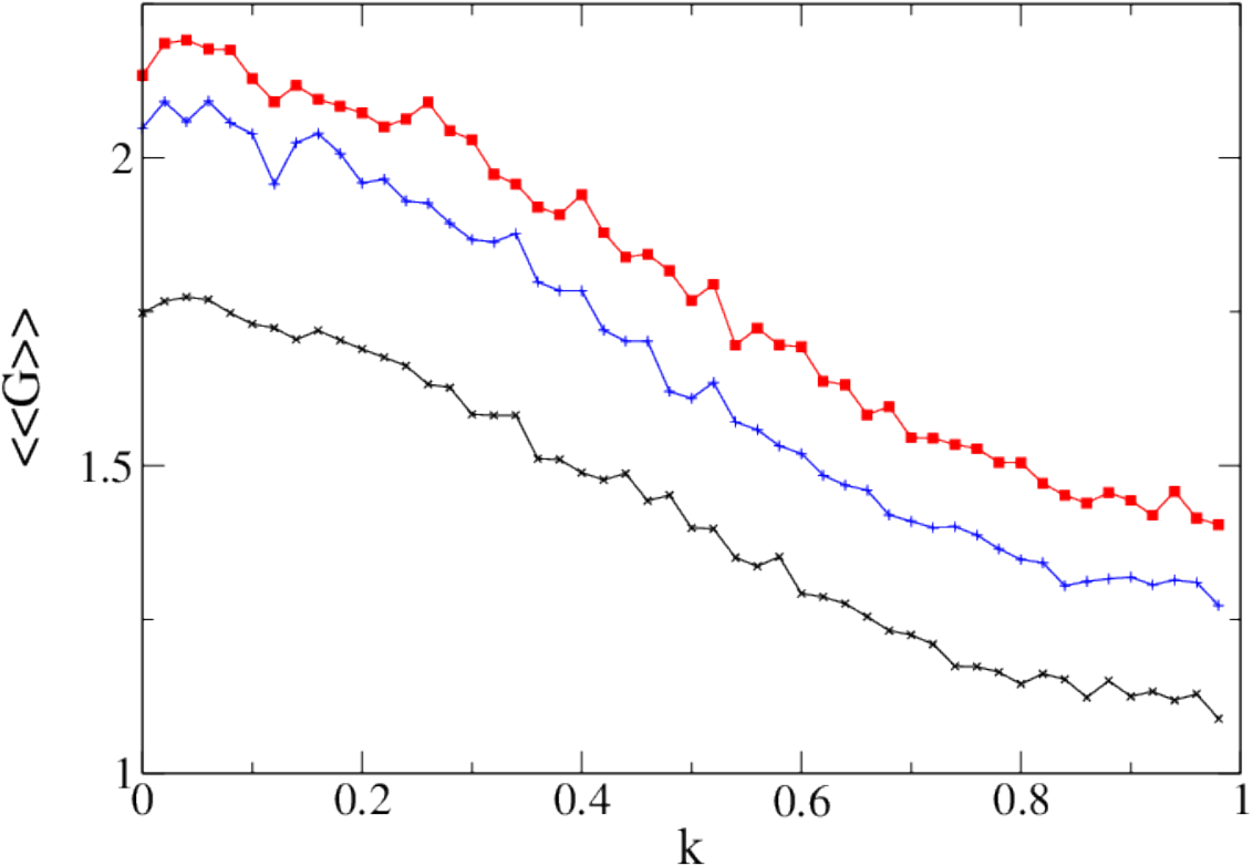
One sees that becomes ever smaller as increases over the complete range of values of , confirming the predictions of the above theoretical analysis. As the coupling is increased from 0, an increasing number of effective star-like networks embedded in the scale-free network become active in the sense that their hubs are the only nodes undertaking a significative amplification of their responses on average. This is the weak coupling regime where the scale-free network’s dynamics can therefore be understood from that of a star-like network. Also, the first relative maximum of of the scale-free network as a function of coupling was systematically found at the value predicted from the star-like network analysis for the only active hub (the most connected) existing at (see Fig. 2, top panel). By increasing slightly from yields the additional activation of the second most connected node such that there are now two effective star-like networks which have, for sufficiently large, a high probability of being isolated each other. Since the averaged amplification of a star-like network exhibits a single maximum as a function of the coupling which is very sharp (cf. Eq. (9)), when the averaged amplification of the most connected hub drastically decreases with respect to its value at , while the averaged amplification of the second most connected hub should also be relatively small owing to its lower number of leaves. This explains the existence of the aforementioned first relative maximum at since the averaged amplification of the scale-free network is no more than the sum of the averaged amplifications of the most connected hubs provided that is sufficiently large. Further increase of yields the activation of additional subsequent most connected nodes resulting in an increasing value of the averaged amplification since these hubs still remain unconnected each other (note the appearance of a secondary relative maximum at a value irrespective of the value of , cf. Fig. 2, top panel).

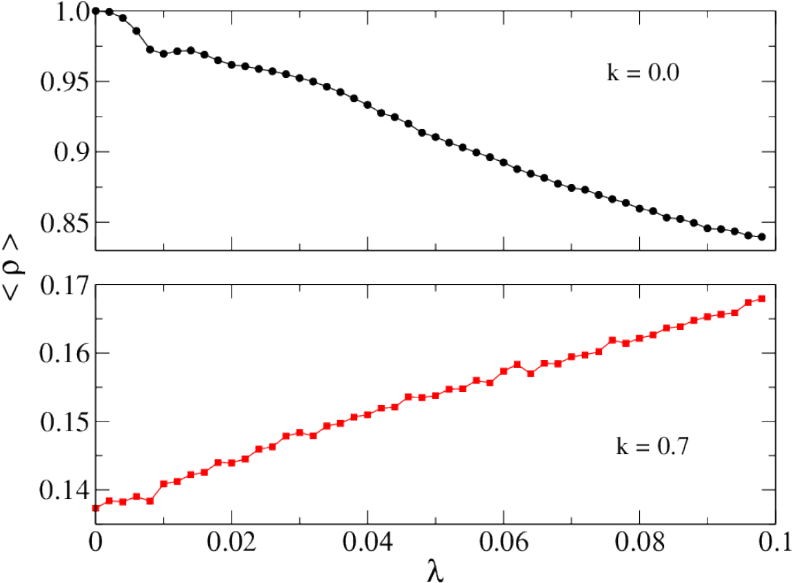
We found that these two first relative maxima appear at (approximately) the same values of in any random realization of the network connectivity and for any value of (see Fig. 3, top panel). This robustness of the amplification scenario against the presence of phase disorder does not hold for the synchronization scenario in the weak coupling regime in the sense that the synchronization monotonously decreases (increases) as is increased from 0 in the absence (presence) of phase disorder (see Fig. 3, bottom panel). This can be understood as the result of two cojoint mechanisms: the disorder-induced lowering of amplification and the coupling-induced increasing of synchronization. Indeed, in the absence of the former mechanism , the latter mechanism by itself is not enough to dominate the desynchronization effect of the topology-induced amplification mechanism. We additionally found that, for any value of the phase disorder parameter , the averaged amplification (synchronization) decreases (increases) as the power-law distribution exponent is increased (see Fig. 4), providing thus an additional confirmation of the robustness of the topology-induced amplification mechanism against the presence of phase disorder.

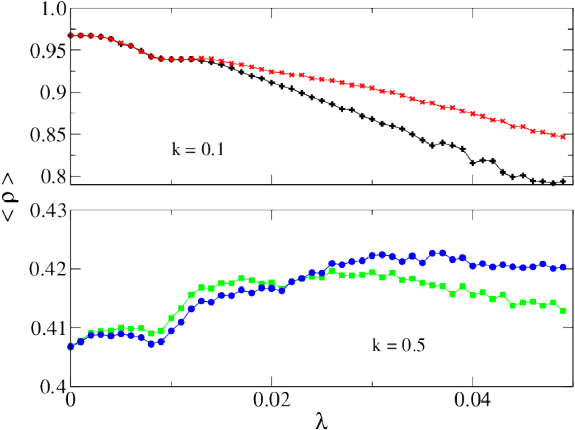
Figure 5 provides an additional example for a higher average degree confirming the above amplification-synchronization scenario. Also, the range of the weak coupling regime where a noticeable amplification occurs diminishes as the average degree is increased irrespective of the strength of phase disorder (see Fig. 5).
IV IV. CONCLUSION
In sum, we have shown through the example of a network of overdamped bistable systems that phase disorder in the external signals strongly reduces topology-induced signal amplification in scale-free networks. We have analytically demonstrated that this effect of quenched temporal disorder may be completely characterized in the simple case of a starlike network. The relevance of the present results stems from the fact that phase disorder in the external signals, contrary to the effect of additive Gaussian white noise [20] and contrary to what happens in regular networks [21,22] of chaotic nonautonomous oscillators where phase disorder acts favouring signal-induced regularization, has a negative effect in the amplification process of external signals, favouring thus synchronization in scale-free networks. Interestingly, our results indicate that the presence of phase disorder does not significantly change the values of the coupling strength where amplification is maximum in its absence (i.e., when all nodes are synchronously driven), which means that the topology-induced amplification mechanism is robust against this kind of quenched disorder. One is thus tempted to speculate that this robustness might well provide another reason for the prevalence of scale-free networks in nature.
We wish to express our gratitude to Prof. J. Gómez-Gardeñes for helpful discussions. R. C. and P. J. M. acknowledge financial support from the Ministerio de Economía y Competitividad (MECC, Spain) through FIS2012-34902 and FIS2011-25167 projects, respectively. R. C. acknowledges financial support from the Junta de Extremadura (JEx, Spain) through project GR10045.
References
- [1] S. N. Dorogovtsev and J. F. F. Mendes, Evolution of networks: From biological nets to the Internet and WWW (Oxford Univ. Press, Oxford, 2003).
- [2] A.-L. Barabási and R. Albert, Science 286, 509 (1999).
- [3] R. Albert and A.-L. Barabási, Rev. Mod. Phys. 74, 47 (2002).
- [4] G. Caldarelli, Scale-free Networks: Complex Webs in Nature and Technology (Oxford Univ. Press, Oxford, 2007).
- [5] M. A. Serrano, D. Krioukov, and M. Boguñá, Phys. Rev. Lett. 100, 078701 (2008); Phys. Rev. Lett. 100, 199002(E) (2008).
- [6] V. Colizza, A. Flammini, M. A. Serrano, and A. Vespignani, Nat. Phys. 2, 110 (2006).
- [7] Y.-Y. Liu, J.-J. Slotine, and A.-L. Barabási, Nature 473, 167 (2011).
- [8] T. Nepusz and T. Vicsek, Nat. Phys. 8, 568 (2012).
- [9] E. López, S. V. Buldyrev, S. Havlin, and H. E. Stanley, Phys. Rev. Lett. 94, 248701 (2005).
- [10] L. Donetti, P. I. Hurtado, and M. A. Muñoz, Phys. Rev. Lett. 95, 188701 (2005).
- [11] C. Zhou and J. Kurths, Phys. Rev. Lett. 96, 164102 (2006).
- [12] Y. Chen, E. López, S. Havlin, and H. E. Stanley, Phys. Rev. Lett. 96, 068702 (2006).
- [13] H. Zhou and R. Lipowsky, Proc. Natl. Acad. Sci. U.S.A 102, 10052 (2005).
- [14] J. A. Acebrón, S. Lozano, and A. Arenas, Phys. Rev. Lett. 99, 128701 (2007); Phys. Rev. Lett. 99, 229902(E) (2007).
- [15] X. Liang, Z. Liu, and B. Li, Phys. Rev. E 80, 046102 (2009).
- [16] T. Kondo, Z. Liu, and T. Munakata, Phys. Rev. E 81, 041115 (2010).
- [17] J. Zhou, Y. Zhou, and Z. Liu, Phys. Rev. E 83, 046107 (2011).
- [18] P. Balenzuela, P. Rué, S. Boccaletti, and J. García-Ojalvo, New J. Phys. 16, 013036 (2014).
- [19] F. C. Leone, L. S. Nelson, and R. B. Nottingham, Technometrics 3, 543 (1961).
- [20] J. A. Acebrón, S. Lozano, and A. Arenas, in Applications of Nonlinear Dynamics, edited by V. In, P. Longhini, and A. Palacios (Springer-Verlag, Berlin, 2009), p. 201.
- [21] Y. Braiman, J. F. Lindner, and W. L. Ditto, Nature (London) 378, 465 (1995).
- [22] R. Chacón and P. J. Martínez, Phys. Rev. Lett. 98, 224102 (2007).