Towards Logical Architecture and Formal Analysis of Dependencies Between Services
Abstract
This paper presents a formal approach to modelling and analysis of data and control flow dependencies between services within remotely deployed distributed systems of services. Our work aims at elaborating for a concrete system, which parts of the system (or system model) are necessary to check a given property. The approach allows services decomposition oriented towards efficient checking of system properties as well as analysis of dependencies within a system.
Index Terms:
formal methods; static analysis; dependencies between services; decomposition; verificationI Introduction
This approach originated from the analysis of two case studies from automotive area, which were developed together with industrial partners within DenTUM and Verisoft-XT11 1 Verisoft-XT project – http://www.verisoftxt.de/ projects. The first case study [1], developing an Adaptive Cruise Control system with Pre-Crash Safety functionality, was motivated and supported by DENSO Corporation, the second case study [2], developing a Cruise Control System with focus on system architecture and verification, was supported by Robert Bosch GmbH. One of the essential questions we have investigated during this analysis was which part of the system functionality do we need to analyse to check a certain property in sense of monitoring, testing or formal verification. In most cases, we don’t need complete information about the system as a whole to analyse certain aspects or to check certain properties. The problem is how to find which local information (at the level of one or more components or subsystems) is sufficient for this check, and how to solve this problem on a formal level to allow the automatisation of the analysis.
The reason for this question has a very practical ground: any additional information about the system can make the whole process slower, more expensive or even infeasible, especially if we are speaking about verification. In the case of model checking this can lead to the state explosion problem. In the case of theorem proving this can lead to stack overflow or excessive or prohibitive amounts of time needed by verification engineers to complete the task.
On the logical level, this problem can be reformulated as follows: What is the minimal part of model needed to check a specific property? We suggest an approach focusing on data and control flow dependencies between services. Dependencies’ analysis results in a decomposition that gives rise to a logical system architecture, which is the most appropriate for the case of remote monitoring, testing and/or verification.
In the case where the check of properties depends on information in one location, obviously we can check the property without remote connection and without sending system-wide data for inclusion in the monitoring, testing, or verification process. In the case of remote connection, an additional problem arises through the need of transferring large amounts of data, for example from sensor instruments or automated test generators and model checkers. Thus, it is crucial to analyse regarding to efficiency, which properties (or their parts) should be checked locally, and which should be sent to the cloud. Therefore, an appropriate model covering all these aspects of remotely deployed distributed systems is needed to fulfil the corresponding constraints and to make decisions on (logical) service-oriented system architecture at least semi-automatically.
Contributions: In this paper, we present a formal approach that allows modelling of data and control flow dependencies between services. The aim of the approach is to allow decomposition oriented towards efficient checking of system properties, also taking into account such characteristics as performance, worst-case execution time, reliability, etc. Another contribution of this approach is a semi-automatic support of these ideas on verification level. Applying ideas introduced in this paper within specification and proof methodology [3], and taking into account human factor analysis [4, 5], we obtain concise and at the same time readable specifications. To support this approach on verification level, we have built the corresponding set of theories in Higher-Order Logic. It allows to check dependency relations using an interactive theorem prover Isabelle/HOL [6]. To discharge proof goals automatically, we apply Isabelle’s component Sledgehammer [7] that employs resolution based first-order automatic theorem provers (ATPs) and satisfiability modulo theories (SMT) solvers.
II Inter-/Intraservice Dependencies
In this paper, we follow the definition of services introduced in [8], where a service is defined as a partial function from input streams to output streams . Thus, the behaviour of a service can be defined partially (only for a subset of its possible inputs), in contrast to the totality of a component interface behaviour. In our approach, we need only an abstract definition of a service: we focus on the analysis of dependencies within and between services, where the behaviour of a (sub)services can be specified using different languages.
While modelling communication between services on a certain abstraction level (i.e. level of refinement/decomposition), we specify the dependencies by the function
|
|
denotes here the set of services at the level . returns for any service the corresponding (possibly empty) set of services that are the sources for the input streams of . More precisely, all the dependencies can be divided into the direct and indirect ones. As a stream we understand here both data and control flows. On the level of logical architecture, we can see a stream as an abstract channel.
Similar to the function , we define direct dependencies by the function
|
|
For example, simply means that at least one of the output channels of is directly connected to some of input channels of . In more complicated situations, we need to reason about the (transient) dependencies within many or all of the services of the system.
The direct sources for can be defined as follows:
|
|
If we do not have to take into account the indirect dependencies, the function is defined to be equal to the function , otherwise we define this function recursively over the set of services using the following fixed point construction:
|
|
The functions and have a number of crucial properties. For example:
(1) If a service does not belong to the set of any service of the system, it also does not belong to the set of any service :
|
|
Thus, if belongs to the set of a service , then exist some service s.t. belongs to its set (as a special case, could also be equal to ):
|
|
This also imply that if set of a service is empty, its set is empty too, and vice versa:
|
|
(2) Transitivity: If a service belongs to the set of a service , which itself belongs to the set of another service , then the service also belongs to the set of a service .
|
|
(3) If we have mutual dependencies between services, then their sets are equal and contain these services themselves ( and denote here some sets over ):
|
|
In general, values of an output channel of a service do not necessarily depend on the values of all its input streams. This means that an optimisation of system/ services’ architecture may be needed in order to localise these dependencies. To express any restrictions we use the following notation: denotes the subset of that depends upon. There are three possible cases to consider:
- •
depends on all input streams of : ;
- •
depends on some input streams of : ;
- •
is independent of any input stream of , i.e.,
.
While determining these sets, we should take into account not only the direct dependence between input/output values, but also the dependence via local variables of the service. For example, let be a service with a local variable , representing its current state, and an output channel , which depends only on the value of . If is updated depending to the input messages the service receives via the input channel , then . To be more precise, we mark this special case by an upper index indicating that influences , and via .
II-A Elementary Services
Based on the definition above, we can decompose services to have for each output channel the minimal sub service computing the corresponding results (we call them elementary services). An elementary service either
- •
should have a single output channel (in this case this service can have no local variables), or
- •
all its output channels are correlated, i.e. mutually depend on the same local variable(s).
Let be a service with input channels
and output channels as well as local variables .
For each output channel , we check the corresponding set :
(1)
If contains only direct dependencies from some input channels, i.e. ,
we remove the corresponding computations from to a single subservice ,
which has a single output channel .
(2)
If contains also dependencies via some local variables, then we
should check which other output channels depend from these variables, because
the output channels depending from the same local variables will belong to the same subservice of , otherwise we will need duplicated computation for these variables.
Thus, we proceed as follows:
- •
If is the only output channel depending from these variables, we remove the corresponding computations from to a single subservice , which has a single output channel .
- •
If there are other output channels depending from these variables, we remove the corresponding computations from to a single subservice , which has output channels .
For all three cases, becomes a set of input channels of the new subservice . If after this decomposition a single service is too complex, we can apply the decomposition strategy presented in [9].
II-B Running Example
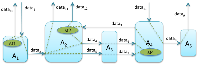
Let us illustrate the presented ideas by an example: we show how each service can be decomposed to optimise the dependencies within each single service, and after that we optimise the architecture of the whole system. Given a system (cf. also Fig. 1) consisting of five services, where the set on the level is defined by . The sets of data and control flow dependencies between the services are shown in Table I. We represent the dependencies graphically using dashed lines over the service box.
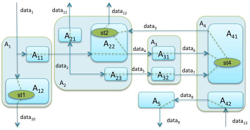
Now we can decompose the system’s services according to the given specification. This results into the next abstraction level of logical architecture (cf. Fig. 2), on which all services are elementary:
-
has two output channels, depending on the input channel directly and depending on the same input channel but via a local variable . Therefore, it should be decomposed in two subservices: with input and output , and with input and output .
-
has four output channels: and depend on the input channel directly, the corresponding computations should be removed to two subservice, and , respectively. depends on the input channel via local variable , but there is another output channel depending on this local variable, therefore, computations for these two outputs should belong to the same subservice . Thus, should be decomposed in three subservices.
-
has two output channels, depending on the input channel directly and depending on the input channel directly. Therefore, it should be decomposed in two subservices.
-
has two output channels, and . It should be decomposed in two subservices, because depends on the input channel directly and depends on the input channels and via local variable .
-
has only one output channel, which means that no decomposition on this level is needed.
III Reliability Analysis and Tracing
The functions and allow us to trace back which parts of the system provide information to a certain service. This provides a basis for identifying of elementary services and the corresponding optimisation of the logical architecture. To trace which services are affected by the results produced by the service, we introduce another two functions, and . For any service , the function (dual to ) returns the corresponding set of output channels depending on input . This help us to solve following problems:
- •
if there are some changes in the specification, properties, constraints, etc. for , we can trace which other channels can be affected by these changes;
- •
having for each output channel the minimal subservice computing the corresponding results, we can check the critical paths in the system by allocating to each subservice /output channel the corresponding worst case execution time (WCET). For this purpose we can use representation of the system architecture as a directed graph (cf. Section IV).
If the input part of the service’s interface is specified correctly in the sense that the service does not have any “unused” input channels, the following relation will hold:
|
|
On each abstraction level of logical architecture, we can define a function . For any service (name) the function returns the corresponding (possibly empty) set of services (names) that are the acceptors for the output streams of . This function dual to the function :
|
|
This model allows us to analyse the influence of a service’s failure on the functionality of the overall system: if a service fails, the set of affected function will be . For example, for the system from Fig. 2, on the abstraction level the services , , , have no acceptors, where the set of acceptors of the service is . Thus, failure of the service causes wrong behaviour only of itself, where failure of the service has influence on the results of seven services (including ). On this basis, we can mark each service by a number of services which are affected by (and, respectively, by its failure). Thus, the impact number of the service will be 1 (the minimal value), where the impact number of will be 7. Moreover, on this basis we can apply results of our previous work on efficient hazard and impact analysis for automotive mechatronics systems [10], which was done in collaboration with industrial partners from ITK Engineering AG.
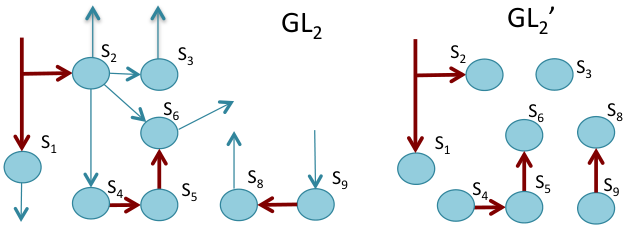
The representation of dependencies between services by a directed graph (like on Fig. 3) allows also to find the worst case execution time (WCET) needed for the concrete output based on the WCETs of the system’s services, as well as analyse the influence of a service’s failure on overall system. For example, from Fig. 3 it is easy to see that for the outputs of the services and the worst case computation time is equal to the WCETs of these services, for the output of the services the worst case computation time is equal to the sum of WCETs of and , etc.
IV Strongly Connected Services
After the decomposition discussed in the previous section, we obtain a (flat) architecture of system. The main feature of this architecture is that each output channel (within the system) belongs the minimal subservice of a system computing the corresponding results.
We represent this (flat) architecture as a directed graph and apply one of the existing distributed algorithms for the decomposition into its strongly connected services, e.g. FB [11], OBF [12], or the colouring algorithm [13]. For our goals, we extend them by a preliminary simplification of the graph (cf. below). This optimisation is algorithm independent and is also applicable for the case another decomposition is chosen.
Let us introduce some basic terms and definitions to explain the main ideas of the decomposition we apply in our approach. A directed graph is a pair , where is a set of vertices, and is a set of directed edges. If , then is called an successor of , and is called predecessor of . A vertex is called reachable from vertex if , where is a transitive and reflexive closure of . If is reachable from , then there is a sequence of vertices (called path), such that for all .
A set of vertices is strongly connected if for any vertices holds that is reachable from . A strongly connected service (SCS) is a maximal straggly connected set of vertices, i.e. after extension of this set by any additional vertex the set is no more strongly connected. An SCS is trivial if it consists of a single vertex. We call an SCS leading (terminating) trivial if it consists of a single vertex that has no predecessors (successors).
In our representation of a flat architecture as a directed graph, services become vertices and channels become edges. We distinguish here
- •
channels that are system’s input/output (within the graph, we represent them by dashed edges, cf. also Fig. 3, because they are less important on this level of (de)composition – we do not need to take them into account by identifying the SCSs), and
- •
channels that are local for the system, i.e. representing dependencies between services.
Vertices that are leading trivial SCSs are labeled by LT, vertices that are terminating trivial SCSs are labeled by TT, and vertices that are commonly trivial SCSs (trivial, but neither leading nor terminating) are simply labeled by T. In addition, we define another special king of trivial SCSs: services that has neither successors, no predecessors (this means that all their input/output channels are system’s input/output channels). We call them disconnected trivial SCSs and label by DT.
Two vertices and of an undirected graph are connected if there is a path from to (for the case of directed graph we need to ignore the orientation of its edges); otherwise, they are disconnected. A graph is connected if every pair of vertices in is connected; otherwise, it is called disconnected. If the graph representing a flat system’s architecture is disconnected, i.e. consists of graphs that are either connected graphs or single vertices (we denote this set by ), then we identify SCSs in each of these graphs separately and could also parallelise these computations (cf. also example below).
Thus, we start the service (de)composition by construction the set from the system’s architecture on level . In the case is connected, we simply have . Then for each graph we proceed as follows:
(1) We identify DT services and delete these vertices from the graph. This is non-recursive procedure with time complexity , where is a number of vertices.
(2) We apply the recursive elimination technique One-Way-Catch-Them-Young (OWCTY, [14]) to remove the LT services and the reversed OWCTY technique to remove the TT services.
(3) The removed services become single services on the level . To the rest of the graph, we apply one of the existing algorithms for the decomposition into SCCs (FB [11], OBF [12], etc.).
To illustrate these ideas, we continue with the example from previous section. We represent the system from Fig. 2 as a directed graph to apply a decomposition algorithm, cf. Fig. 3. This graph is disconnected and consists of two connected graphs, and , therefore we can analyse them in parallel. For we need to perform the following steps:
(1) First of all, we identify as a DT service, delete it from the graph (system’s subservice on the level ).
(2) Then, we apply the OWCTY elimination techniques to identify and remove the LT and TT services:
- •
On the first run of the algorithm, we identify and as an LT and an TT services respectively and delete them. They become and on the level .
- •
After this, (which is commonly trivial in ) becomes an LT service and should be deleted, becoming on . Then, the same situation will be with : it should be deleted as an LT service and becomes .
- •
The rest of the graph (vertices , , ) with corresponding edges contains neither LT nor TT vertices. This is an input for the SCC-decomposition algorithm.
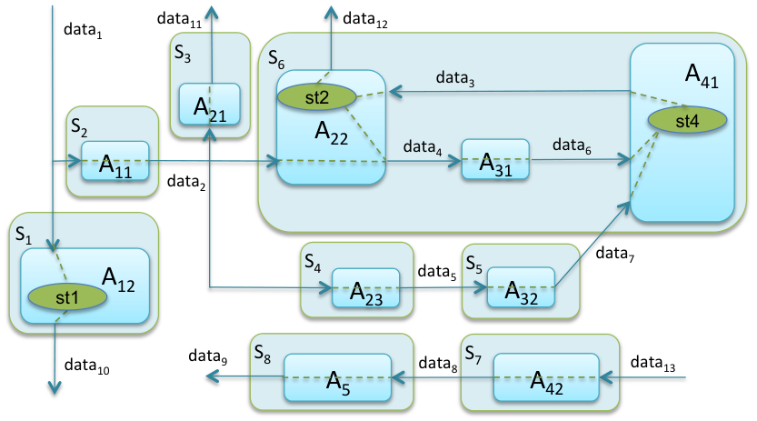
(3) In our example we apply a variant of the FB algorithm. The time complexity of this algorithm is , where is a number of vertices and is the number of edges in this graph. The FB algorithm identifies that the vertices , , build a single SCS, which becomes on the level . has only two vertices, a leading trivial SCS and a terminating trivial SCS . Thus, on the level it gives us two subservices of the system: and . Fig. 4 presents the result of the architecture optimisation.
V Efficient Checking of Properties
A property can be represented by relations over data and control flows on the system’s channels. Let for a relation , and be the sets of input and output channels of the system used in this relation. For each channel from we recursively compute all the sets of the dependent input channels. Their union, restricted to the input channels of the system (for the case we exclude properties’ specification over local channels), should be equal to , otherwise we should check whether the property was specified correctly (i.e. exclude (human) error in the specification of the property, e.g., when a wrong channel identifier was used) and if so, precise it or eliminate unnecessary constraints:
(1) If a channel belongs to but not to , we need to extend explicitly specifying that this property should hold for any values on .
(2) If a channel belongs to but not to , this means that is unnecessary strict, because it contains assumptions on irrelevant input channel.
From we obtain the set of services having these channels as outputs, compute the union of corresponding sets . This union together with give us the minimal part of the system needed to check the property . This allowed us, especially in the case of cloud-supported processing, to reduce the costs of monitoring, testing or verification.
Assume we have to check relation specified for the system presented on Fig. 4. It is easy to see, that there is no dependency between and . We have here and . is a single output channel of , i.e. . This gives us . Thus, which is already equal to , because is a system input. First of all we need to exclude error in the specification of the property, e.g. the case where is meant to be specified over and . If was specified without such errors, we need (1) to extend it explicitly specifying that it should hold for any values on , and (2) eliminate unnecessary constraints on from . Because , we need only the service to check this property.
Assume now we have to check relation specified for the same system.
For this case and .
is a single output channel of , and therefore .
(both channels are local), .
, which gives us (this is a system input channel, therefore it should be a part of ).
.
, (also local), .
, (local, cf. above), .
, there is no need to extend the property or eliminate some to its constraints.
To check this property we need the following set of services:
.
VI Remote Computation
In the previous section we have analysed, which part of the overall information about the system and its input data is necessary to check the corresponding property. In the similar way, we can trace the influence of the system environment’s properties on the properties of the system itself. However, the decision, which information need to be processed locally (local services) and which need to be sent to the cloud (remote services), should be made not only according to this analysis of a (logical) system architecture, but also taking into account the following aspects of data flows between services:
(1) measure for costs of the data transfer/ upload to the cloud UplSize(f): size of messages (data packages) within a data flow and frequency they are produced. This measure can be defined on the level of logical modelling, where we already know the general type of the data and can also analyse the corresponding service (or environment) model to estimate the frequency the data are produced;
(2) measure for requirement of using high-performance computing and cloud virtual machines, Perf(X): complexity of the computation within a service , which can be estimated on the level of logical modelling as well.
On this basis, we build a system architecture, optimised for remote computation. We associate an UplSize measure to each channel (to each data flow), and an Perf measure to each elementary service in the system (i.e. for any service on the abstraction level ). A limit, above which a remote computation is desired, is denoted by HighPerf. A limit of the UplSize measure, above which a limited up-/download is desired, is denoted by HighLoad, i.e. if the source of the data is deployed locally then the receiving services should preferably also deployed locally, and i.e. if the source is deployed in the cloud then the receiving services should preferably also deployed in the cloud. We do not take into account costs of the transfer of software service themselves, assuming that this aspect is already covered by the Perf measure. The UplSize measure should be analysed only for the channels that aren’t local for the services on abstraction level .
Using graphical representation, we denote channels with UplSize HighLoad by thick red arrows, and the services with Perf HighPerf by white colour, where all other channel and services are marked blue. We use the same colouring notation when building the corresponding tables for the values above limits as well as when represented a system by the corresponding directed graph. For the compressed table representation, which allows readable representation of the large systems’ measures, we omit the concrete values of the measures leaving only the notes on relations to the defined limits. While measuring Perf on the level , we mark a service by a sum of Perf measures of its subservices on the level . Thus, if the Perf measure of at least one subservice is high, the same hold for the service’s Perf.
This analysis can also be done automatically, provided all the measures UplSize and Perf are defined for data and control flows as well as for (elementary) services. Using our approach, we can prove a number of properties for service composition according to these measures. We start with the architecture from abstraction level and represent it as a directed graph. Then we simply remove edges that correspond to channels with low UplSize, and obtain a set of connected graphs. If any two vertices (or graphs) are “connected” by a single edge that is “split” and has no source vertex (this represents a situation where a system input goes to many systems’s services), we see them as a connected graph too. Each of the graphs becomes a service on the abstraction level represents a system architecture, optimised for remote computation.
Assume the following case for the system from the previous examples (cf. also Fig. 4):
- •
channels with UplSize value HighLoad:
, , , , , . - •
services with Perf value HighPerf: , , , , and on the abstraction level : , , , .
and are local channels of , their UplSize measure is not relevant for this case. We represent the system from the abstraction level as a directed graph (cf. Fig. 5). After removing edges that correspond to channels with low UplSize, we obtain a set of connected graphs.

Fig. 6 represents a system architecture, optimised for remote computation. On the abstraction level (cf. Fig. 6), and are composed together into a new service : corresponds to a data flow, where messages (data packages) have large size and come with a high frequency, but has very low frequency (e.g., realise a filtering function according to a given criteria), therefore it make more sense to deploy locally, together with .
There are no changes for service , but , , and are composed into , and with into . The services and have Perf measure higher HighPerf, therefore using high-performance computing and cloud virtual machines is required for these services.
VII Semi-Automatic Formal Verification
To support this approach on verification level, we have also build a set of corresponding theories in Higher-Order Logic (HOL) using an interactive semi-automatic theorem prover (proof assistant) Isabelle [6]. This proof assistant is based on polymorphic HOL extended with axiomatic type classes, and support the proof of arbitrary mathematical theorems in interactive manner. Proofs are constructed in the structured proof language Isar [15]. The advantage of this proof language is that the proofs are easy readable for both human and machine, which is not the case for many proof languages.
The representation of our approach in Isabelle/HOL contains approx. 70 general axioms and lemmas [16], which are necessary to analyse dependencies within a system using Isabelle in (semi-)automatic way, e.g. to verify whether a given set of services is equal to the set of (in)direct sources of some service, or whether the set of services is equal to the minimal set needed to check a certain property. To show a feasibility of the approach, we also have done a case study using our formalisation. In this case study [16], we started with 9 services connected with 24 channels on the abstraction level (among them 4 services are specified using local variables). Fig. 7 presents how the number of services was changed among the abstraction levels.

Overall, the case study contains more than 300 lemmas, approx. 50% of them can be composed and proven automatically, using the predefined schema, which is a part of our formalisation. All the technical details of formalisation within the theorem prover Isabelle as well as the corresponding proofs for a case study to elaborate the approach are presented in [16]. Approx. 90% of the proofs (general as well as for a concrete system from the case study) are constructed using Isabelle’s component Sledgehammer [7]. Sledgehammer discharges proof goals applying to them resolution based first-order automatic theorem provers (ATPs) and satisfiability modulo theories (SMT), which makes the human-related part of the proof simpler and faster.
VIII Discussion and Related Work
The approach presented above extends our previous work in [1, 2, 9] by providing formal approach that allows modelling of (data and control flow) dependencies between components, and associated algorithm for architecture optimisation towards efficient verification, testing, and monitoring of system’s properties. We leave here out of scope the automatisation of the construction of the functions , , etc. for a concrete case. For the example presented in this paper as well as for the case study, verified in Isabelle, these functions were specified manually. Thus, this automatisation is planned for the future work. However, one of the advantages of our current work is formal semi-automatic analysis of system architecture, and the sufficiency of the set of system’s components to check a certain property. Thus, in our work we touch the following research areas: modelling communication between components, system decomposition, as well as architecture modelling. In the rest of the section we discuss the related work on them.
Modelling communication:
Various languages and techniques have been proposed to represent
communication between components/processes, for example, Bergstra’s
Algebra of Communicating Processes [17], Hoare’s approach on
Communicating Sequential Processes [18] and its extension
[19]. Magee et al. [20] tried to
combine the ideas of operational semantics with Milner’s
calculus, calculus of mobile processes
(cf. [21, 22]). Reo, a channel-based coordination
model for component composition, represents a co-algebraic view on
this area [23, 24].
The work presented in [25] defines an extensive support to the components communication and time requirements, while the model discussed in [26] proposes general ideas on model for distributed automation systems.
Our approach, in contrast, is focusing not on the communication in general but on the dependency aspects and how their analysis can be used to increase the efficiency of properties checking.
System decomposition.
There is a large number of approaches in the area of systems
decomposition (see, e.g., [27, 28]). In general we can say, that decomposition in many cases leads to a
refinement of a system, where by composing a system from components we
can implicitly build a new level of abstraction of system
representation (cf. [29, 30]).
The main difference and
the main contribution of our current work, also compared with our previous work
on formal decomposition [9], is an
extension of the specification approach to associate
subspecifications with subservices or architectural components in a
more usable, readable way,
focusing on the aspects essential for the efficient checking of system’s properties, taking into account aspects that are important
for the case of using high-performance computing and cloud virtual machines.
To this end, our focus in the current paper goes
also beyond ideas presented in [9], where
readability and manageability of specification were discussed in relation
to inconsistencies and incomplete specifications.
Architecture modelling.
An introductory overview of foundations and applications of the model
driven architecture can be found in [31].
There is a large collection of approaches on architecture elaboration,
with different aims and domain orientations, e.g.,
Medvidovic and Taylor [32] introduce a classification and
comparison framework for software architecture description
languages, Malek et al. [33]
presents a framework for improving distributed system’s architecture
and their deployment,
Broy et al. [8] focus on specification and design of services
and layered architectures.
A number of approaches, e.g., [34], propose several meta-models that introduce relationships between architectural design decision
alternatives and activities related to them.
A number of architecture description languages have been
developed to specify compositional views of a system on an abstract
level, e.g., TrustME [35], which
combines software architecture specification approaches with ideas of
design-by-contract and allows capturing of
behavioural interaction patterns
between large-scale components of software and systems architectures.
Our current work is focused on modelling of a logical service-oriented architecture. The main focus of our approach is on
elaborating for a concrete system, which part of the system is sufficient to check a certain property, and how to optimise the logical architecture towards efficient monitoring, testing, and verification of system’s properties, also for the case of remote connection.
IX Conclusion and Future Work
In this paper, we presented a formal approach to modelling and analysis data and control flow dependencies between components. We described the theory which lies behind the approach and presented a running example to illustrate the main ideas of the approach. We conclude that our approach allows
- •
to specify the dependencies within a system formally,
- •
to elaborate for a concrete system, which part of the system is sufficient to check a certain property,
- •
to analyse tracing and reliability aspects,
- •
to optimise the architecture of a given system, also taking into account such aspects as costs of data transfer/ upload to the cloud, and requirements of using high-performance computing and cloud virtual machines,
These results are especially important for analysis and optimisation of remotely deployed distributed control systems: our approach allows system decomposition oriented towards efficient checking of system properties – it allows to send to or from the cloud only the information really needed for the monitoring, testing or verification of the properties of interest.
Another contribution of our approach is a semi-automatic support of the presented ideas on verification level, an interactive semi-automatic theorem prover Isabelle/HOL.
Future Work: In the future work, we intent to automatise the construction of the functions that specify the dependencies (, , etc.) for a concrete case on each level of abstraction. One of the other possible directions of our future work is on combination of the ideas presented above with our previous work on analysis of crypto-based components [36], to analyse the data dependencies between components wrt. secrecy/security properties.
References
- [1] M. Feilkas, F. Hölzl, C. Pfaller, S. Rittmann, K. Scheidemann, M. Spichkova, and D. Trachtenherz, “A Top-Down Methodology for the Development of Automotive Software,” TU München, Tech. Rep. TUM-I0902, 2009.
- [2] M. Spichkova, “Architecture: Methodology of decomposition,” TU München, Tech. Rep. TUM-I1018, 2010.
- [3] ——, “Stream Processing Components: Isabelle/HOL Formalisation and Case Studies,” Archive of Formal Proofs, 2013, Formal proof development.
- [4] ——, Design of formal languages and interfaces: “Formal” does not mean “unreadable”, K. Blashki and P. Isaias, Eds. IGI Global, 2013.
- [5] ——, “Human Factors of Formal Methods,” in In IADIS Interfaces and Human Computer Interaction 2012. IHCI 2012, 2012.
- [6] T. Nipkow, L. C. Paulson, and M. Wenzel, Isabelle/HOL – A Proof Assistant for Higher-Order Logic, ser. LNCS. Springer, 2002, vol. 2283.
- [7] J. C. Blanchette, S. Böhme, and L. C. Paulson, “Extending Sledgehammer with SMT solvers,” in Automated Deduction, ser. LNCS, N. Børner and V. Sofronie-Stokkermans, Eds., vol. 6803. Springer, 2011, pp. 116–130.
- [8] M. Broy, “Service-oriented Systems Engineering: Specification and design of services and layered architectures. The JANUS Approach,” Engineering Theories of Software Intensive Systems, pp. 47–81, 2005.
- [9] M. Spichkova, “Architecture: Requirements + Decomposition + Refinement,” Softwaretechnik-Trends, vol. 31:4, 2011.
- [10] S. Dobi, M. Gleirscher, M. Spichkova, and P. Struss, “Model-based hazard and impact analysis,” TU München, Tech. Rep. TUM-I1333, 2013.
- [11] L. Fleischer, B. Hendrickson, and A. Põnar, “On identifying strongly connected components in parallel,” in Parallel and Distributed Processing, ser. LNCS, J. Rolim, Ed. Springer, 2000, vol. 1800, pp. 505–511.
- [12] J. Barnat, J. Chaloupka, and J. van de Pol, “Improved distributed algorithms for scc decomposition,” Electron. Notes Theor. Comput. Sci., vol. 198, no. 1, pp. 63–77, 2008.
- [13] S. M. Orzan, “On distributed verification and verified distribution,” Ph.D. dissertation, Free University of Amsterdam, 2004.
- [14] K. Fisler, R. Fraer, G. Kamhi, M. Vardi, and Z. Yang, “Is there a best symbolic cycle-detection algorithm?” in Tools and Algorithms for the Construction and Analysis of Systems, ser. LNCS, T. Margaria and W. Yi, Eds. Springer, 2001, vol. 2031, pp. 420–434.
- [15] M. Wenzel, “The isabelle/isar reference manual,” 2013.
- [16] M. Spichkova, “Formalisation and analysis of component dependencies,” Archive of Formal Proofs, 2014, Formal proof development.
- [17] J. A. Bergstra and J. W. Klop, “Algebra of communicating processes with abstraction,” Theor. Comput. Sci., vol. 37, pp. 77–121, 1985.
- [18] C. A. R. Hoare, “Communicating sequential processes,” Commun. ACM, vol. 21, no. 8, pp. 666–677, Aug. 1978.
- [19] G. Hilderink, “Graphical modelling language for specifying concurrency based on csp,” IEEE: Software, vol. 150, pp. 108–120, 2003.
- [20] J. Magee, N. Dulay, S. Eisenbach, and J. Kramer, “Specifying distributed software architectures,” in Proceedings of the 5th European Software Engineering Conference. Springer, 1995, pp. 137–153.
- [21] R. Milner, A Calculus of Communicating Systems. Springer, 1982.
- [22] ——, Communicating and mobile systems - the Pi-calculus. Cambridge University Press, 1999.
- [23] F. Arbab, “Reo: a channel-based coordination model for component composition,” Mathematical Structures in Computer Science, vol. 14, pp. 329–366, 6 2004.
- [24] S. Meng, F. Arbab, B. Aichernig, L. Astefanoaei, F. de Boer, and J. Rutten, “Connectors as designs: Modeling, refinement and test case generation,” Science of Computer Programming, vol. 77, no. 7-8, 2012.
- [25] B. Vogel-Heuser, F. S., T. Werner, and C. Diedrich, “Modeling network architecture and time behavior of distributed control systems in industrial plant,” in 37th Annual Conference of the IEEE Industrial Electronics Society, ser. IECON, 2011.
- [26] T. Hadlich, C. Diedrich, K. Eckert, T. Frank, A. Fay, and B. Vogel-Heuser, “Common communication model for distributed automation systems,” in 9th IEEE International Conference on Industrial Informatics, ser. IEEE INDIN, 2011.
- [27] J. Philipps and B. Rumpe, “Refinement of Pipe-and-Filter Architectures,” in FM’99, J. M. Wing, J. Woodcock, and J. Davies, Eds., no. LNCS 1708. Springer, 1999, pp. 96 – 115.
- [28] D. B. da Cruz and B. Penzenstadler, “Designing, Documenting, and Evaluating Software Architecture,” TU München, Tech. Rep. TUM-I0818, 2008.
- [29] M. Broy, “Compositional refinement of interactive systems,” ACM, vol. 44, no. 6, pp. 850–891, 1997.
- [30] M. Spichkova, “Refinement-based verification of interactive real-time systems,” Electronic Notes in Theoretical Computer Science, vol. 214, pp. 131–157, 2008.
- [31] A. Rensink and J. Warmer, Eds., Model Driven Architecture - Foundations and Applications, ser. LNCS, vol. 4066. Springer, 2006.
- [32] N. Medvidovic and R. Taylor, “A classification and comparison framework for software architecture description languages,” IEEE Trans. Softw. Eng., vol. 26, no. 1, pp. 70–93, 2000.
- [33] S. Malek, N. Medvidovic, and M. Mikic-Rakic, “An extensible framework for improving a distributed software system’s deployment architecture,” IEEE Trans. Software Eng., vol. 38, no. 1, pp. 73–100, 2012.
- [34] J. Tyree and A. Akerman, “Architecture decisions: demystifying architecture,” Software, IEEE, vol. 22, no. 2, pp. 19–27, 2005.
- [35] H. Schmidt, I. Poernomo, and R. Reussner, “Trust-by-contract: Modelling, analysing and predicting behaviour of software architectures,” J. Integr. Des. Process Sci., vol. 5, no. 3, pp. 25–51, Aug. 2001.
- [36] M. Spichkova, “Compositional properties of crypto-based components,” Archive of Formal Proofs, 2014, Formal proof development.